Optimization of Location-Routing for Multi-Vehicle Combinations with Capacity Constraints Based on Binary Equilibrium Optimizers

Abstract

The Location-Routing Problem (LRP) becomes a more intricate subject when the limits of capacities of vehicles and warehouses are considered, which is an NP-hard problem. Moreover, as the number of vehicles increases, the solution to LRP is exacerbated because of the complexity of transportation and the combination of routes. To solve the problem, this paper proposed a Discrete Assembly Combination-Delivery (DACA) strategy based on, the Binary Equilibrium Optimizer (BiEO) algorithm, in addition, this paper also proposes a mixed-integer linear programming model for the problem of this paper. Our primary objective is to address both the route optimization problem and the assembly group sum problem concurrently. Our BiEO algorithm was designed as discrete in decision space to meet the requirements of the LRP represented by the DACA strategy catering to the multi-vehicle LRP scenario. The efficacy of the BiEO algorithm with the DACA strategy is demonstrated. through empirical analysis utilizing authentic data from Changchun City, China, Remarkably, the experiments reveal that the BiEO algorithm outperforms conventional methods, specifically GA, PSO, and DE algorithms, resulting in reduced costs. Notably, the results show the DACA strategy enables the simultaneous optimization of the LRP and the vehicle routing problem (VRP), ultimately leading to cost reduction. This innovative algorithm proficiently tackles both the assembly group sum and route optimization problems intrinsic to multi-level LRP instances.

1. Introduction

It is crucial for a reasonable logistics system design to reduce the total cost of the supply chain and improve supply efficiency. In order to achieve the above two objectives, it is usually necessary to determine two levels of decision-making: the immediate determination of facility location problems (FLP) and the vehicle routing problem (VRP) [1]. Historically, researchers usually treated these as two types of decisions separately.

The FLP stands as a quintessential quandary within the realm of operations research. This locational puzzle has an extensive array of applications spanning production, daily life, and logistics such as establishments of factories, warehouses, first aid centers, and logistics hubs. Hu et al. [2] employed a multi-objective mixed integer model in their investigation to ascertain the optimal siting of hazardous goods recycling stations, accounting for traffic constraints on urban roads. The efficacy of their approach was substantiated through solving a real-world case study on hazardous material logistics in Shandong, China. In the work of Oksuz et al. [3], a two-stage stochastic model was harnessed to tackle the location challenge posed by temporary medical centers. By factoring in patient types, requirements, potential road and hospital damage, along with the distances between disaster areas and hospitals, the model methodically sought optimal solutions for temporary hospital placements. This model was then practically employed in selecting a suitable site for a temporary hospital during an Istanbul disaster. Additionally, Karagöz et al. [4]. leveraged the ARAS extended interval type-2 fuzzy model to resolve the location quandary for vehicle recycling centers, juxtaposing it against the conventional interval type-2 fuzzy approach to underscore the potency of the ARAS method. Nonetheless, in practical scenarios, a challenge will emerge after the identification of suitable facility sites: the optimization of vehicle routes to effectively serve customers within the designated coverage area. This challenge aligns with long-term decision-making imperatives.

The second vital factor in a logistics system design is the VRP. According to references [5,6,7], different VRPs have different mathematical models, and mixed integer linear programming is often used to solve problems. According to the client’s ordering demand with a certain capacity-limited set of vehicles, the appropriate travel routes from the logistics center to the clients are organized so that the vehicles pass through all the clients in an orderly manner to reach a certain goal under the satisfaction of certain constraints (e.g., demand, service time limitation, vehicle capacity limitation, mileage limitation, etc.). Qin et al. [8] used the original heuristic algorithms based on reinforcement learning for the vehicle path problem with a multi-vehicle fleet of different capacities and tested on a large dataset, achieving an average GAP of 6.4% compared to the classical algorithms of PSO, GA, and SA; Altabeeb et al. [9] proposed a cooperative hybrid firefly algorithm for solving the vehicle routing problem with capacity constraints and tested it on 108 benchmark cases, achieving an average GAP of 3.4% compared to HAHA and 4.9% compared to LNS-ACO. Rabbouch et al. [10] solved the enriched vehicle routing problem with time window and pause time constraints using an efficient implementation of a genetic algorithm, which was able to complete the enriched vehicle path problem 1–17 min faster than the GA’s CPU response time depending on the size of the algorithm.

The FLP and the VRP were usually addressed separately, although they are mutually influenced and restrained. This disjointed approach would fail to achieve an overarching optimal solution due to the lack of integration between these two critical aspects. The significance of their integration was underscored by Maranzana et al. [11] and Webb et al. [12], prompting a shift towards combining these problems. Consequently, the fusion of FLP and VRP has gained prominence, leading to the emergence of the Location-Routing Problem (LRP) propelled by advancements in optimization technology. LRP is an NP hard problem [13]. In [14], Muñoz-Villamizar et al. designed an integer linear programming model for urban logistics, which solved the problem of logistics center positioning and distribution in cities and achieved a distance cost lower limit of 20.77%. In [15], Heidari et al. proposed a mixed integer linear programming to solve the transportation problem of hazardous materials. In a small case with 2 nodes and 3 retailers, the solution only took 0.19 s. In [16], Shaerpour et al. designed a multi-layer multi-objective mixed integer linear programming model to solve the management and transportation of medical waste, and demonstrated the effectiveness of the proposed model in a practical case in Tehran. This confluence has ushered in a surge of research into LRP. Cao et al. [17] introduced a two-stage mixed integer model for the procurement of farm crops and the ensuing two-stage LRP involving processing facilities. Similarly, Biuki et al. [18] tackled the two-level LRP inherent to perishable goods supply chains. Their hybrid heuristic algorithm, integrating genetic and particle swarm optimization algorithms, outperformed traditional meta-heuristic methods across a comprehensive benchmark assessment. The burgeoning interest in LRP is evident in the work of Ferreira et al. [19], which highlights the increasing attention directed towards this problem.

In practical applications, the LRP often focuses on the Capacitated Location-Routing Problem (CLRP), which is tightly bound by stringent vehicle capacity constraints. Specifically, the determination of warehouse locations and vehicle routes exhibits a mutual interdependence. The chosen warehouse locations exert a profound influence on subsequent vehicle route planning, while the resultant vehicle route plans inherently reflect the efficacy of the warehouse location selection. A previous study [13] employed nested methodologies for an iterative resolution of location and routing predicaments. This involved the locator sequentially identifying sets of warehouses, followed by the routing program’s endeavor to optimize routes based on the designated warehouses. However, the above approach faces limitations in that vehicle paths corresponding to distinct warehouse assemblies tend to operate independently, impeding the effective utilization of valuable historical vehicle routing insights.

To seek better and more effective methods for the CLRP, meta-heuristic algorithms were applied in recent years. This idea found practicality in the study by Ferreira et al. [19], where a hybrid meta-heuristic algorithm was employed to resolve the CLRP, yielding superior outcomes compared to conventional solutions. Furthermore, Akpunar et al. [20] addressed the CLRP using a broad domain search algorithm, albeit without incorporating combinatorial assembly optimization for multi-vehicle fleets at the VRP stage. It is found that there are two key points to using meta-heuristic algorithms to solve CLRP. Firstly, since the solution of CLRP is a combinatorial problem, finding an appropriate expression of the solution in the decision space becomes the key to the problem. The second is that since CLRP involves location selection and combinatorial path optimization, its solution space has continuous and discrete characteristics, so selecting appropriate meta-heuristic algorithms is also a key element.

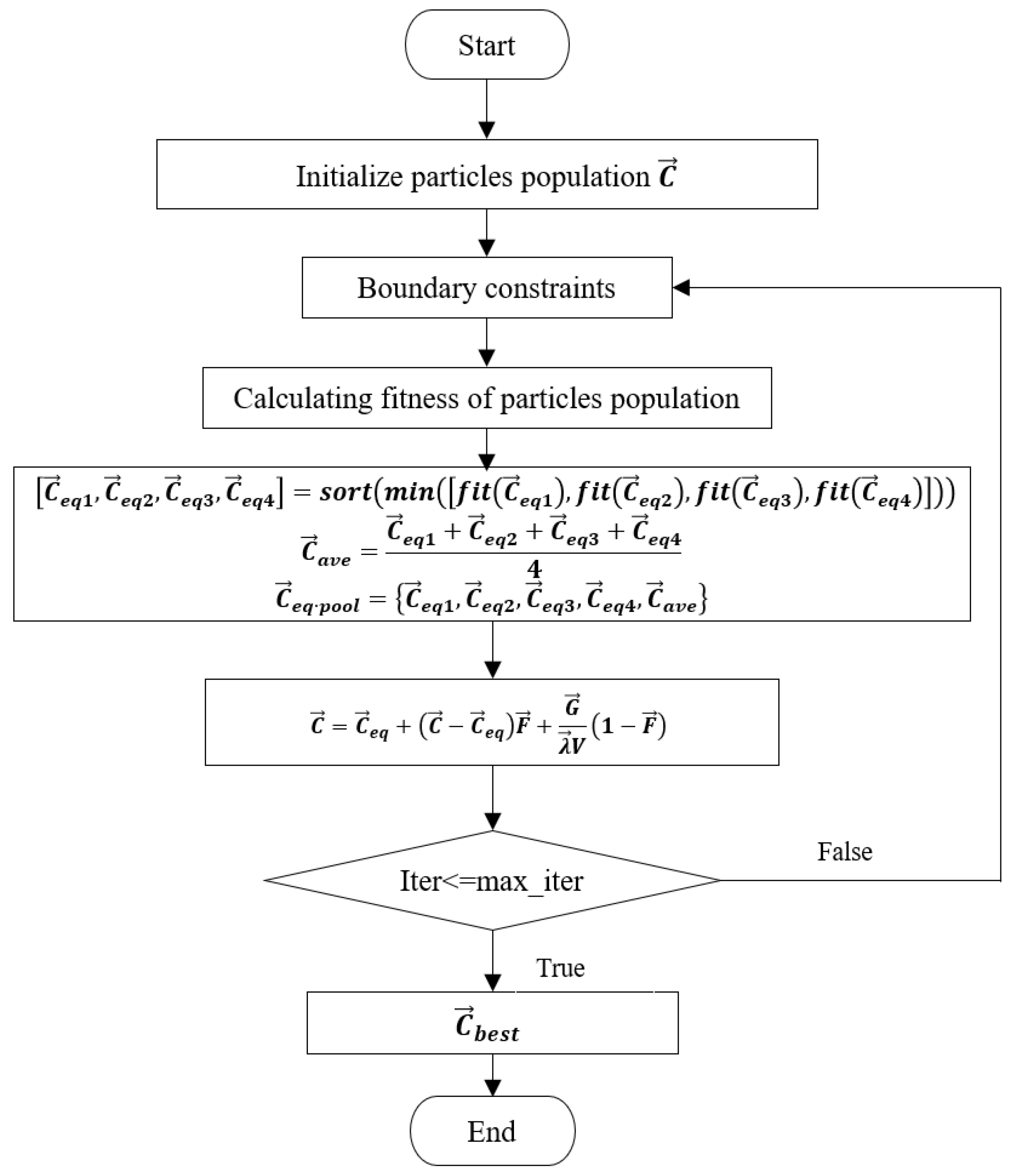
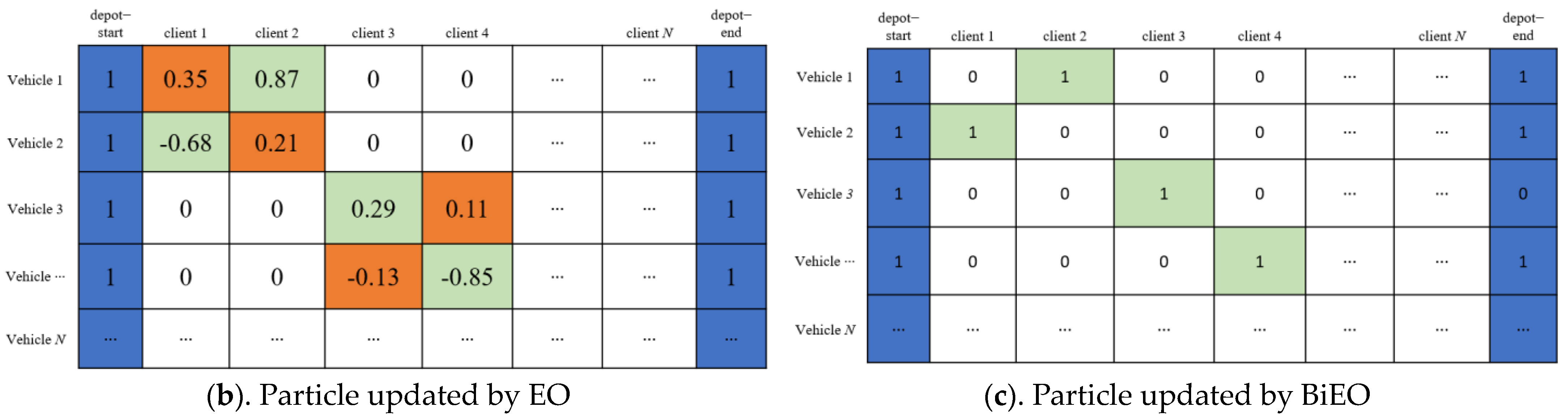
To optimize the assembly combination of multi-vehicle during vehicle path optimization by considering constraints of the CLRP, this paper proposed the BiEO algorithm with a multi-vehicle decision set for the assembly combination of multi-vehicle routing.

Table 1. Comparison of this paper’s problem and algorithm with other papers.

Papers	Algorithm	FLP	VRP	CLRP	Combination
Karagöz et al. [4]	ARAS	✓	✗	✗	✗
Qin et al. [8]	RLHH	✗	✓	✗	✗
Altabeeb et al. [9]	CVRP-CHFA	✗	✓	✗	✗
Rabbouch et al. [10]	GA *	✗	✓	✗	✗
Ting et al. [21]	MACO	✓	✓	✓	✗
Vincent et al. [22]	SA	✓	✓	✓	✗
Zhang et al. [23]	HPSO	✓	✓	✓	✗
Peng et al. [24]	PSO	✓	✓	✓	✗
Yu et al. [25]	HGA	✓	✓	✓	✗
This paper	BiEO	✓	✓	✓	✓

shows the comparison of this paper’s problem and algorithm with other articles.

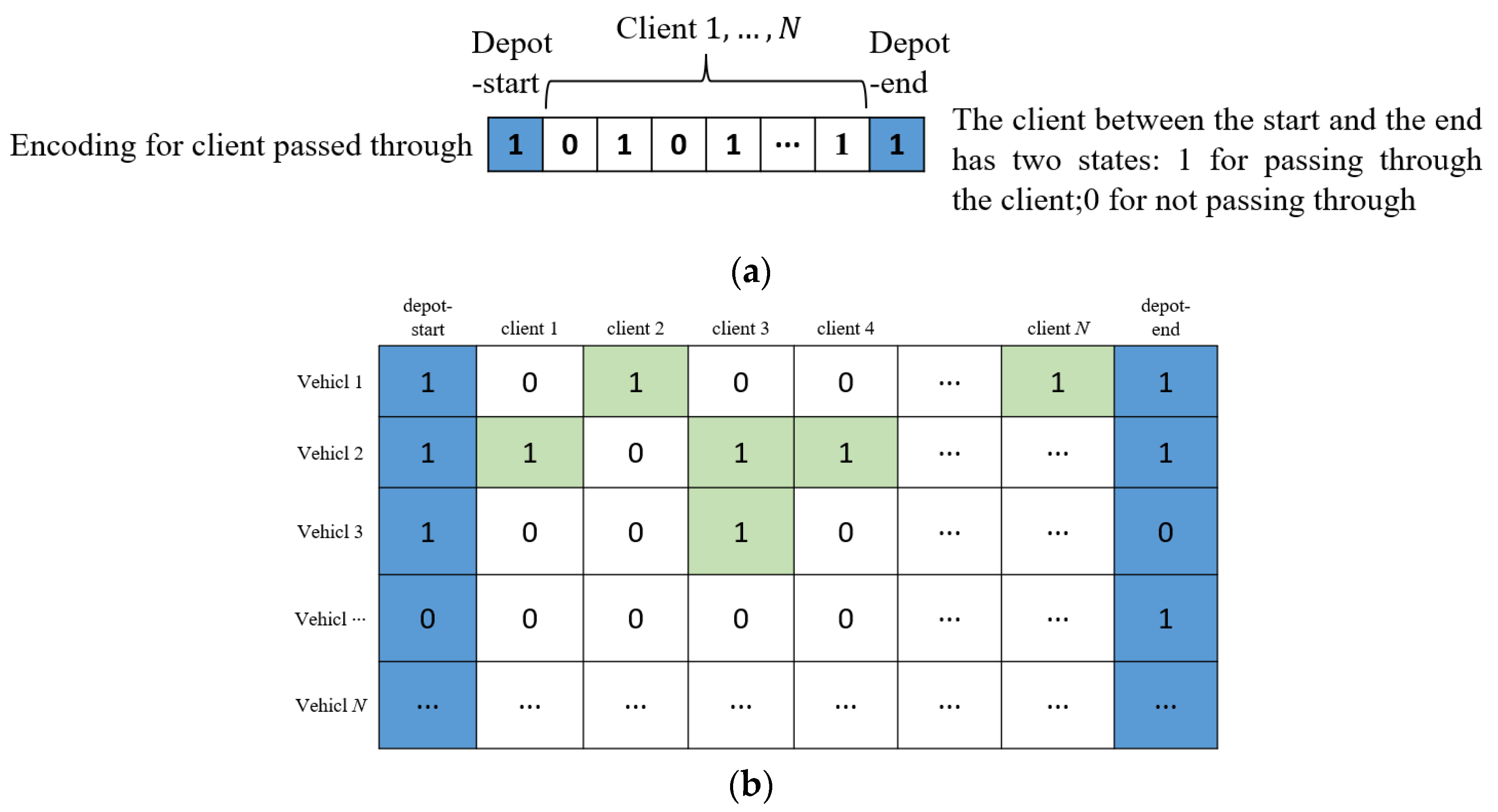
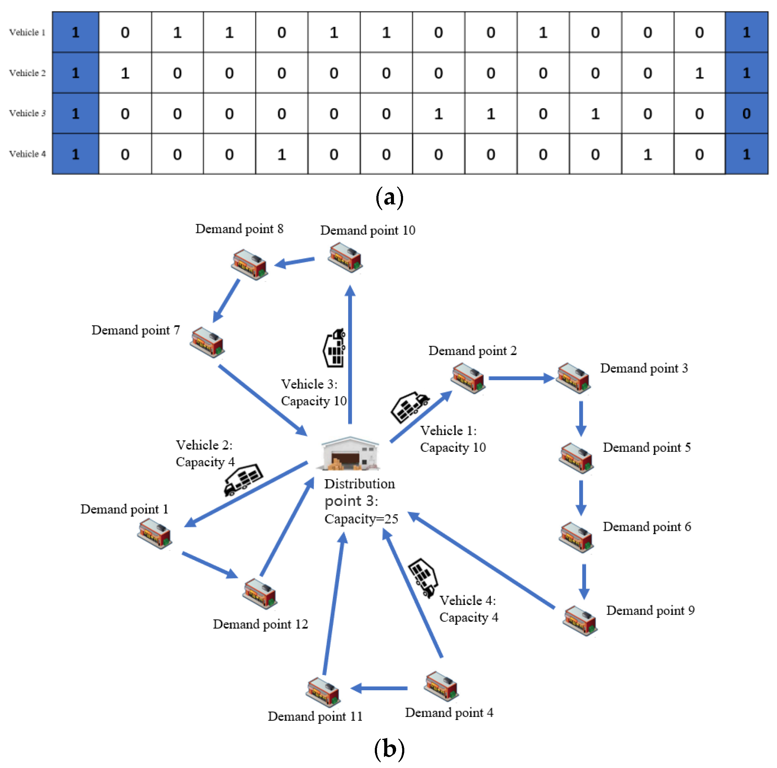
This paper needs to optimize the location of warehouses for material storage in residential areas with a population of about 300,000 (assuming a fixed daily material demand of 400 g per resident) and optimize the transportation routes for subsequent truck transportation of materials. This is an LRP problem, and it is worth noting that in the transportation route optimization problem in this article since each distribution area uses four trucks to transport goods, it is necessary to optimize the assembly of goods on the trucks before planning the transportation route. The model and method proposed in this paper are used to solve the problem of simultaneously assembling and transporting routes on trucks. The final solution solved in this paper is the assembly plan and transportation route for each truck in each distribution area.

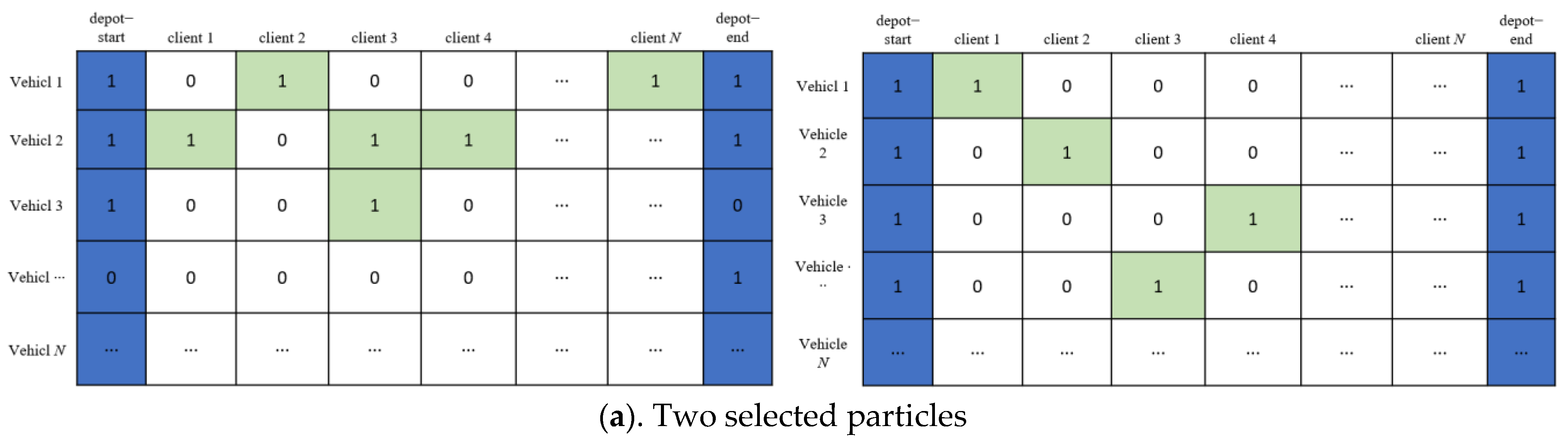
The contribution of this paper is that firstly, it proposes a BiEO algorithm that can effectively solve the route optimization problem in this paper. Secondly, this paper proposes a DACA strategy to solve the assembly combination and route optimization problems of multiple vehicles in this paper. The two methods proposed in this paper have achieved better results in solving real LRP compared to other algorithms in the experiment.

The initial section provides an introduction to FLP, VRP, and LRP, especially CLRP. The subsequent section delves into a comprehensive review of pertinent prior research, in which emphasis was placed on introducing various variants of LRP, as well as precise methods and heuristic and meta-heuristic methods for solving LRP. In the third section, we designed the framework and formal problem statement of the Binary Equilibrium Optimizer (BiEO). At the same time, the DACA strategy was proposed to solve multi-vehicle routing problems. Moving on, the fourth section Introduced the LRP mathematical model proposed in this paper to solve the case study. The fifth section offers an extensive exposition of empirical findings derived from applying the proposed BiEO algorithm to real-world scenarios. Lastly, the sixth section engages in a comprehensive discussion of the results and implications of this study’s contributions.

2. Related Work

2.1. Variants of LRP

The multi-level LRP is an important variant of the LRP, which involves a distribution system integrating warehouses, intermediate warehouses, and retailers. Investigating the multi-level LRP holds the potential to significantly curtail distribution costs and enhance turnover efficiency, thereby conferring substantial importance to its study. In 2012, Nguyen et al. [26] addressed the two-level LRP employing the GRASP technique. This approach encompassed intermediate warehouse localization, path optimization from warehouse to intermediate warehouse, and further optimization from intermediate warehouse to retailer. The incorporation of GRASP facilitated enhanced solutions through its iterative learning process and path re-linking mechanism. Subsequently, Nguyen extended this work by embracing a multi-starting approach, coupling the ILS + PR algorithm [27], enriched with enhancements such as greedy random heuristics and diverse short-term tabu lists, culminating in improved outcomes. Nevertheless, it’s important to note that such enhancements may incur elevated computational time.

Another variant of the LRP is characterized by randomness and fuzziness, denoting the consideration of uncertainties and ambiguities in customer requirements during logistics route planning. These uncertainties are often amenable to modeling through stochastic, probabilistic, or fuzzy functions. Ghaffari-Nasab et al. [28] tackled a two-objective LRP involving probabilistic travel times, offering both modeling and solution strategies. An enhanced particle swarm optimization algorithm was presented to fulfill the random demands in LRP scenarios [23]. Thereafter, Zarandi et al. [29] proposed an analog embedding simulated annealing algorithm as a solution approach in the context of the multi-site CLRP with fuzzy travel times.

The CLRP stands as a prevalent variation within the broader LRP framework, where warehouse capacity, depot capacity, vehicle load, and other relevant factors are subject to constraints [20]. Due to the complexity of combinatorial solutions and the diversity of constraint conditions, traditional path optimization is difficult to achieve. Therefore, researchers are attempting new ways to solve this problem. Yu et al. devised an innovative Hybrid Genetic Algorithm (HGA) [25], adept at exploring between feasible and infeasible solution domains, yielding commendable outcomes when applied to solving the CLRP involving warehouse capacity limitations. Building upon this, Akpunar et al. [20] introduced a hybrid meta-heuristic approach, fusing Adaptive Large Neighborhood Search (ALNS) and Variable Neighborhood Search (VNS) algorithms. In this composite framework, the VNS algorithm serves as an elite local search mechanism, thus amplifying the efficacy of the ALNS algorithm. Consequently, the proposed hybrid meta-heuristic approach seamlessly integrates diversification and intensification strategies through the distinctive merits of the ALNS and VNS algorithms, respectively. The meta-heuristic approach provides a new approach to solving CLPR problems, which requires finding appropriate meta-heuristic algorithms and solution structures for the practical CLPR.

2.2. CLRP Solution

2.2.1. Precise Solution

A precise solution for CLRP is to use mathematical methods to find the optimal solution for CLRP. In 2011, Belenguer et al. [30] introduced a branch and cut methodology for CLRP, employing a customized set of valid inequalities within a 0–1 linear model. Their approach effectively ascertained optimal solutions, particularly suitable for instances involving up to 40–50 customers and 5 potential warehouses. Shortly thereafter, Baldacci et al. [31] proposed an alternate precise technique grounded in the set partitioning formulation of CLRP, broadening its applicability to a wider spectrum of optimization scenarios. Their strategy entails decomposing the challenge into a finite collection of Multi-Depot Vehicle Routing Problems (MDVRP) through lower bounds established by diverse boundary programs. Contardo et al. [32] expanded the scope by introducing meticulous methods founded on cutting and column generation techniques. It’s important to acknowledge, however, that the potency of precise methods tends to diminish as the complexity of the problem escalates. This is evident in instances such as the 40-customer cases documented in [33], where the resolution process can extend over several hours.

2.2.2. Heuristic and Meta-Heuristic Solution

Owing to the formidable computational intricacies and heightened complexity entailed in addressing large-scale CLRP problems through precise methodologies, the research focus has gravitated towards heuristics and meta-heuristics. Prins et al. [34] devised the Greedy Stochastic Adaptive Search Program (GRASP), a dual-component approach encompassing warehouse location acquisition and subsequent path refinement, effectively resolving the CLRP challenge. Extending this work, Duhamel and Prins et al. [35] introduced GRASP × ELS, an evolution of GRASP wherein evolutionary local search (ELS) superseded conventional local search. Ting et al. [21] proposed a Multi-Ant Colony Optimization algorithm (MACO) that dissects CLRP into three distinct sub-problems—warehouse selection, customer allocation, and vehicle routing. The algorithm deployed three ant colony iterations tailored to these sub-problems, consistently exhibiting superior or near-optimal performance across benchmark instances. Vincent et al. [22] harnessed Simulated Annealing Heuristics (SA) for CLRP, encoding solutions as lists and repositories as sub-lists. Employing pseudo-zeros, routes were iteratively combined, building upon an initial solution generated through the greedy approach and subsequently refined via local search. A similar SA encoding was presented by Jokar et al. [36], wherein the initial solution underwent refinement through a dual-stage process involving greedy initialization and subsequent local search. In another vein, a pragmatic and effective Hybrid Genetic Algorithm was introduced by Lopes et al. [37], employing route representation and featuring specialized route copy crossover and two mutation operators “add”, and “swap”. Moreover, distinct local search routines were tailored for depot location and route enhancement.

On the basis of the implementation of the meta-initiation algorithm in the CLPR problem, researchers have further improved its solution accuracy. Quintero-Araujo et al. [38] introduced a partial stochastic meta-heuristic algorithm to address CLRP, culminating in a solution that demonstrated a 0.4% improvement over the classical BKSS reference solution. In parallel, Peng et al. [24], leveraging the Particle Swarm Optimization algorithm (PSO), achieved a 2.4% enhancement over the classical BKSS solution when dealing with a test set involving 20 customers and 5 warehouses. Furthermore, Zhang et al. [23] crafted a hybrid heuristic grounded in the PSO algorithm, tailored for CLRP scenarios with fuzzy requirements. This approach yielded outcomes notable for their stability when compared to CPLX-based solutions.

However, combinations arising from multi-vehicle transportation in the VRP phase have not been considered in previous CLRP work.

3. Location-Routing Optimization with Capacity Based on BiEO

The difficulties in solving the multi-vehicle distribution route combination scheme with capacity constraints are: 1. The number of demand points that each group of vehicles passes through is different due to the different transportation ranges of each distribution point; 2. Since there are capacity constraints on the vehicles and they are transported in multi-vehicle mode, there exists an optimization problem for the combination of assemblies for each group of vehicles prior to transportation. Therefore, studying optimization algorithms that are suitable for delivery needs and formulating decision plans for multi-vehicle delivery is crucial.

To address the challenges inherent in the assembly combination optimization and route optimization of multi-vehicle fleets within LRP, this paper proposed the Binary Equilibrium Optimizer (BiEO) and binary combination list solution for multi-vehicles to satisfy the multi-vehicle combination distribution problem with capacity constraints.

3.1. Equalization Optimizer

The Equilibrium Optimizer (EO) [39], introduced by Afshin Faramarzi et al. in 2019, stands as an optimization algorithm, drawing inspiration from the hybrid dynamics of mass balance physics with a robust control volume. At its core lies the mass balance equation, capturing the intricate physical processes that govern mass entry, exit, and generation within the defined volume. Notably, the EO effectively surmounts the challenge of converging to local optima, achieved through its implementation of a candidate pool mechanism and the multi-directional updating attributes. When juxtaposed against genetic algorithms and particle swarm optimization algorithms, the Equilibrium Optimizer boasts heightened optimization prowess and swifter convergence rates. The algorithmic workflow of EO is depicted in Figure 1.

The EO algorithm is different from other algorithms in that it has an equilibrium pool mechanism that allows for better global and local development performance. The equilibrium pool is generated according to Formulas (1)–(3).

$$\left[{\overrightarrow{C}}_{eq1},{\overrightarrow{C}}_{eq2},{\overrightarrow{C}}_{eq3},{\overrightarrow{C}}_{eq4}\right]=sort\left(\min \left(\left[fit\left({\overrightarrow{C}}_{eq1}\right),fit\left({\overrightarrow{C}}_{eq2}\right),fit\left({\overrightarrow{C}}_{eq3}\right),fit\left({\overrightarrow{C}}_{eq4}\right)\right]\right)\right)$$

(1)

$${\overrightarrow{C}}_{ave}=\frac{{\overrightarrow{C}}_{eq1}+{\overrightarrow{C}}_{eq2}+{\overrightarrow{C}}_{eq3}+{\overrightarrow{C}}_{eq4}}{4}$$

(2)

$${\overrightarrow{C}}_{eq·pool}=\left\{{\overrightarrow{C}}_{eq1},{\overrightarrow{C}}_{eq2},{\overrightarrow{C}}_{eq3},{\overrightarrow{C}}_{eq4},{\overrightarrow{C}}_{ave}\right\}$$

(3)

The update formula for the EO algorithm is Formula (4).

$$\overrightarrow{C}={\overrightarrow{C}}_{eq}+\left(\overrightarrow{C}-{\overrightarrow{C}}_{eq}\right)\overrightarrow{F}+\frac{\overrightarrow{G}}{\overrightarrow{\lambda }\mathrm{V}}\left(1-\overrightarrow{F}\right)$$

(4)

where $\overrightarrow{F}$ is the exponential term generated by Formula (5); $\overrightarrow{\lambda }$ is assumed to be a random vector in the interval of [0, 1]. $\overrightarrow{G}$ is the generation rate generated by Formula (7).

$$\overrightarrow{F}=a_{1}sign\left(\overrightarrow{r}-0.5\right)\left[e^{-\overrightarrow{\lambda }\mathrm{t}}-1\right]$$

(5)

where is $a_1$ constant value that controls exploration ability; r is a random vector between 0 and 1; t is defined as a function of iteration generated by Formula (6).

$$t={\left(1-\frac{iter}{Max\_iter}\right)}^{\left(a_2\frac{iter}{Max\_iter}\right)}$$

(6)

where $iter$ and $Max\_iter$ present the current and the maximum number of iterations, respectively, $a_2$ is a constant value.

In reference [39], the available values for $a_1$ and $a_2$ are $a_1=\left[1, 1.5, 2, 2.5, 3\right]$, $a_2=\left[0.1, 0.5, 1, 1.5, 2\right]$. In the work of this paper, $a_1$ and $a_2$ have chosen $a_1=2$ and $a_2=1.$

$$\overrightarrow{G}={\overrightarrow{G}}_0\overrightarrow{F}$$

(7)

where ${\overrightarrow{G}}_0$ is the initial value generated by Formula (8).

$${\overrightarrow{G}}_0=\overrightarrow{GCP}\left({\overrightarrow{C}}_{eq}-\overrightarrow{\lambda }\overrightarrow{C}\right)$$

(8)

where $\overrightarrow{GCP}$ generated by Formula (9).

$$\overrightarrow{GCP}=\left\{\begin{array}{c}0.5r_1 r_2\ge GP\\ 0 r_2<GP\end{array}\right.$$

(9)

where $r_1$and $r_2$are random numbers in [0, 1].

EO was applied to reference [40] to enhance the voltage profile in the distribution system by reconfiguring the DG placement through an equalization optimizer algorithm due to its superior accuracy of optimization search and convergence speed than algorithms such as GA and PSO. However, the original EO algorithm’s decision space design proves inadequate for accommodating constraints during the process of path optimization and assembly problem-solving.

3.2. Design and Implementation of BiEO

3.2.1. BiEO

This paper proposed the BiEO to meet the discrete solution of vehicle assembly combination and delivery in the route optimization process, due to the current EO algorithm is designed for continuous domains. BiEO can ensure that the binary population is not destroyed during the update process. The pseudo-code of the BiEO is as follows in Algorithm 1.

Algorithm 1. BiEO

Input: Population size $N$; the maximum number of iterations $\mathrm{M}\mathrm{a}\mathrm{x}\_\mathrm{i}\mathrm{t}\mathrm{e}\mathrm{r}$ Output: Best individual $\overrightarrow{C}$; fitness of $\overrightarrow{C}$ 1: Initialize the partice population ${\overrightarrow{C}}_i^D,i=1,\dots ,N$ 2: Initializes the control parameters $a_1=2, a_2=1, GP=0.5$ 3: While $iter<Max\_iter$ 4:   For $i=1:N$ 5:    calculate ${\overrightarrow{C}}_i$ fitness 6:   End for 7:  sort the particle population and find the first four particles by Formula (1) 8:  calculate ${\overrightarrow{C}}_{ave}$ particles 9:  construct the equilibrium pool by Formula (3) 10:   calculate $t$ 11:   For $i=1:N$ 12:    Randomly choose one candidate from the equilibrium pool 13:    generate randomly vector $\overrightarrow{\lambda }$ 14:    generate $\overrightarrow{F}$, $\overrightarrow{GCP}$, ${\overrightarrow{G}}_0$, $\overrightarrow{G}$ 15:    update particle population by Formula (4) 16:   End(for) 17:  X = abs ($\overrightarrow{C}$) 18:   For $i=1:N$ 19:    For $j=1:dimension of \overrightarrow{C}\left(D\right)$ 20:     $M=\max \left({\overrightarrow{C}}_i^D\right);m=\mathrm{m}\mathrm{i}\mathrm{n}\left({\overrightarrow{C}}_i^D\right)$; 21:     generate random number r $=m+(M-m)\ast rand$ 22:     $\mathrm{P}\left(X_i^j\right)=\frac{X_i^j}{\sum _{k=1}^{\mathrm{D}}{X}_i^k}$ 23:      If $\mathrm{r}<\mathrm{P}\left(X_i^j\right)$ 24:       ${\overrightarrow{C}}_i^D$=1 25:      Else 26:       ${\overrightarrow{C}}_i^D$=0 27:      End if 28:    End for 29:   End for 30:  $iter=iter+1$ 31: End while

3.2.2. The DACA Strategy for Multi-Vehicle Route Optimization

The DACA strategy for multi-vehicles was designed as shown in Figure 2. The Schematic diagram of route coding for a certain distribution point is shown in Figure 2a. In the figure, the depot represents distribution points, and the client represents demand points. A solution for a certain vehicle covers 3 elements: start-depot, client encoding, and end-depot. When the Start-depot is 1, it indicates that the vehicle is selected for delivery; When the nth client is 1, it indicates that the vehicle delivers goods to the nth client. When the end-point is 1, it indicates that the distribution is a feasible sub-solution under the condition of the limited capacity of this vehicle. As a whole feasible solution to the combination multi-vehicles, all sub-solutions should be feasible. The initialization of delivery for multi-vehicles in decision space is shown in Figure 2b. This approach facilitates the concurrent optimization of both the distribution routes for the vehicles at the distribution point and the corresponding vehicle capacities. The DACA strategy not only addresses assembly combination optimization but also effectively abides by the constraints imposed by vehicle capacities.

4. Model of Logistics System for Multi-Vehicles Based on BiEO

4.1. The Model Design Based on BiEO

Our model serves to ascertain the optimal locations and quantities of distribution points, while concurrently devising distribution route schedules between these distribution points and each individual demand point. The overarching objective is to minimize the overall cost while effectively fulfilling the material requisites of each specified demand point. Below, we proceed to provide definitions and elucidations pertaining to the sets, indices, parameters, and decision variables integral to our formulation.

$$\underset{}{\min }Z=\sum _{i\in \mathrm{L}}\sum _{\mathrm{j}\in \mathrm{L}}{V}_{ij}{X}_{ijV}^W{C}_V{d}_{ij}+\sum _{i\in \mathrm{L}}\sum _{\mathrm{j}\in \mathrm{L}}{v}_{ij}{x}_{ijv}^w{C}_v{d}_{ij}$$

(10)

Formula (10) is the optimization objective function and Z is the minimum cost optimization objective. The parameters are described in

Table 2. The solution set of the model.

Set	Description
$V$	Set of large vehicles ($V=1,2,3...V_n$)
$v$	Set of small vehicles ($v=1,2,3...v_n$)
$S$	The number of distribution points ($S=1,2,3...S_n$)
$R$	Set of demand points ($R=1,2,3...R_n$)
$L$	Set of distribution points and demand points ($L\in R\cup S$)

,

Table 3. Variables of the objective function.

Parameter	Definition
$d_{ij}$	The distance from the demand point $i$ to the demand point $j$, $\forall i, j\in L$
$V_{ij}$	The large vehicle from the demand point $i$ to the demand point $j$, $\forall i, j\in L$
$v_{ij}$	The small vehicle from the demand point $i$ to the demand point $j$, $\forall i, j\in L$

,

Table 4. Parameters of the objective function.

Variables	Description	Values
$C_V$	Cost per mile for the small vehicle	100
$C_v$	Cost per mile for the large vehicle	40

and

Table 5. Decision variables of the objective function.

Decision Variables	Description	Values
$X_{ijV}^W$	large vehicle $X$ with $V$ Load limit loads $W$ from the demand point $i$ to the demand point $j$ directly	0 or 1
$x_{ijv}^w$	small vehicle $x$ with $v$ Load limit loads w from the demand point $i$ to the demand point $j$ directly	0 or 1

.

The additional assumptions are the following:

(1)

The number and the capacity of distribution points are subject to defined limitations, which remain inviolable.

(2)

The transport vehicles adhere to capacity constraints, which are to be strictly adhered to.

(3)

Uniformity prevails in the transportation aspect: each distribution point caters to a designated transport area, employing vehicles of the same capacity, type, and uniform unit transport cost.

(4)

Each demand point necessitates a single visit.

(5)

The daily demand at each demand point remains constant. Meanwhile, we assume that each person’s daily demand is fixed at 400 g.

The constraints are shown in the following Formulas (11)–(24).

(1)

Each demand point can only have one distribution point responsible for delivery.

$$\sum _{j\in \mathrm{R}}{u}_{ij}=1 \forall i\in S$$

(11)

where $u_{ij}$ indicates that distribution point $i$ is responsible for the delivery of demand point$j$, $u_{ij}\in \left\{\mathrm{0,1}\right\}$

(2)

The total amount of transported materials is less than the inventory.

$$\sum _{i,j\in R}{w}_{ij}^V{X}_{ijV}^W+\sum _{i,j\in R}{w}_{ij}^v{x}_{ijv}^w-\sum _{i,j\in L}{\tilde{E}}_i{u}_{ij}=0$$

(12)

where $w_{ij}^V$ is the total load w of large vehicles from demand point $i$ to the demand point $j$, $\forall i, j\in L$; $w_{ij}^v$ is the total load w of small vehicles from demand point $i$ to the demand point $j$, $\forall i, j\in L$; ${\tilde{E}}_i$ is the demand of the demand point $i$, $\forall i\in R$; $X_{ijV}^W$is large vehicles load W from demand point $i$ to demand point$j$; $x_{ijv}^w$is small vehicles load w from demand point $i$ to demand point $j$; $w_{ij}^V,w_{ij}^v\geqq 0 \forall i,j\in \mathrm{L},\forall V\in V,\forall v\in v$;$X_{ijV}^W,x_{ijv}^w\in \left\{\mathrm{0,1}\right\}\forall i,j\in L$.

(3)

There is only one kind of vehicles on the transport route to a certain demand point:

$$\sum _{i,j\in L}{X}_{ijV}^W-\sum _{i,j\in L}{X}_{jiV}^W=0$$

(13)

$$\sum _{i,j\in L}{x}_{ijv}^w-\sum _{i,j\in L}{x}_{jiv}^w=0$$

(14)

where $w$ represents the current load of the small vehicle departing immediately; $W$ represents the current load of the large vehicle departing immediately.

(4)

Transport routes can exist in both large vehicles and small vehicles:

$$\sum _{i,j\in L}{X}_{ijV}^W-\sum _{i,j\in L}{x}_{ijv}^w\le 1$$

(15)

Formula (15) indicates that on the same transportation route, it can pass through both large vehicles and small vehicles.

(5)

Return when the vehicle is not enough to meet the demand of the next demand point:

$$\sum _{I,j\in R}{w}_{ij}^V{X}_{ijV}^W-{\tilde{E}}_i\ge 0$$

(16)

$$\sum _{i,j\in R}{w}_{ij}^v{x}_{ijv}^w-{\tilde{E}}_i\ge 0$$

(17)

where ${\tilde{E}}_i$ is the demand for demand point $i$, Formulas (16) and (17) represent the return to the warehouse when the transportation vehicle load does not meet the demand for the next demand point.

(6)

The constraint of the transport starting point and vehicle capacity constraints:

$$\sum _{i\in S}\sum _{j\in R}{w}_{ij}^v{x}_{ijv}^w\le W_v$$

(18)

$$\sum _{i\in S}\sum _{j\in R}{w}_{ij}^V{X}_{ijV}^W\le W_V$$

(19)

where $W_V$ is the maximum load of large vehicles, which is set to 10 in this paper; $W_v$ is the maximum load of small vehicles, which is set to 4 in this paper; Meanwhile, Formulas (18) and (19) indicates that the transportation load of large vehicles and small vehicles cannot exceed their respective load limits.

(7)

Constraints of the transportation terminal:

$$\sum _{i\in R}\sum _{j\in S}{V}_{ij}{X}_{ijV}^W=1$$

(20)

$$\sum _{i\in R}\sum _{j\in S}{v}_{ij}{x}_{ijv}^w=1$$

(21)

(8)

Decision variable constraints:

$$X_{ijV}^W,x_{ijv}^w\in \left\{\mathrm{0,1}\right\}\forall i,j\in L$$

(22)

$$u_{ij}\in \left\{\mathrm{0,1}\right\}\forall i\in S,\forall j\in R$$

(23)

$$w_{ij}^V,w_{ij}^v\geqq 0 \forall i,j\in L,\forall V\in V,\forall v\in v$$

(24)

The Formula (24) indicates that the load of large vehicles and small vehicles cannot be empty.

4.2. The Implement of the Multi-Vehicle Route Optimization

The implement scheme, shown in Figure 3, includes (1) the strategic determination and optimization of distribution point locations, and (2) the formulation of optimal routes originating from each distribution point, directing towards the associated demand point.

5. Experiments

5.1. Data

The data set is sourced from the population distribution in the high-tech zone of Changchun, China. Specifically, the algorithm and model are utilized to establish distribution points within the high-tech zones for material transportation during the COVID-19 lockdown.

The high-tech zone comprises 90 distinct demand points with an approximate population of 300,000 individuals. To achieve the efficient distribution of household supplies to these communities, it is necessary to optimize the location of the distribution points and the driving route from the distribution point to the community. Firstly, due to the varying density of geographical distribution in residential areas and the varying population of each community, it is necessary to establish temporary material distribution points based on the above information. Secondly, within each distribution point, a fleet of four vehicles is available, comprising both large vehicles (with a 10-ton capacity) and small vehicles (with a 4-ton capacity), deployable in diverse combinations as necessitated.

5.2. Algorithm Settings

In this paper, the problem of location and route optimization is simultaneously considered, which means the route optimization problem involves the assembly and combination of four vehicles. Therefore, the simultaneous solution described in this paper focuses on utilizing the DACA strategy proposed in this paper to simultaneously solve the problem of combining vehicle assembly combination and vehicle route optimization.

5.2.1. The Optimization of the Location of Distribution Points by EO

The optimization objective function of the location of distribution points is to minimize the distance from the warehouse to the distribution points as shown in Formula (25). The location of distribution points in this paper is continuous with no pre-elected location of distribution points.

$$\underset{}{\min }D=\sum _{j\in \mathrm{S}}\sum _{i\in \mathrm{R}}{p}_{ij}$$

(25)

where $p_{ij}$ is the distance from the distribution point $i$ to the demand point j.

Another location selection scheme is designed based on the regional population density. Demand points with high population density have bigger weights, which means distribution points’ locations will approach the areas with higher probability. On the contrary, Demand points with low population density will have smaller weights, and distribution points’ location will stay away from areas with high probability. The objective function is shown in the Formula (26).

$$\underset{}{\min }D=\sum _{j\in \mathrm{S}}\sum _{i\in \mathrm{R}}{w_{i}p}_{ij}$$

(26)

where $w_i$ is the weight of demand points $i$. $w_i$ is generated according to Formula (18).

$$w_i=\frac{k_i}{N} , \forall i\in R$$

(27)

where $N$ is the total population within the distribution area. $k_i$ is population of demand point $i$.

5.2.2. The Route Optimization of the Multi-Vehicle by BiEO

The optimization objective function is the lowest distribution cost as shown in Formula (10). In multi-vehicle combination transportation, there are three important constraints: 1. All demand points have to be distributed, Formula (11); 2. The total load of all transportation vehicles must not exceed the demand point’s demand, Formula (12); and 3. The starting and ending points of all transportation vehicles must be distribution points, Formulas (18)–(21). The DACA strategy and BiEO proposed in this paper are utilized in route optimization under multi-vehicle combinations.

The original EO’s population update has the potential to inadvertently breach the constraint that each demand point must be traversed by a single vehicle only once. Figure 4a,b provide an illustrative instance of such an update. In the figure, the depot represents distribution points, and the client represents demand points. In Figure 4a, the two matrices depict the chosen individuals prior to the update, whereas the matrices in Figure 4b portray the outcomes following the population update. Notably, the results displayed in Figure 4b conspicuously violate the stipulated constraint of singular point passage (evident through the emergence of multi-values within the same column), subsequently forsaking their binary-coded 0 s and 1 s representation. Consequently, this renders the accurate evaluation of the fitness function impracticable during subsequent assessments. To address this predicament, enhancements are introduced to the equilibrium optimizer to ensure that the result updates adhere to the prescribed constraint conditions.

5.3. Results

5.3.1. The Optimization Distribution Points by EO

Figure 5 shows the location results of distribution points based on (25) and (26). The red star in Figure 5 represents the optimized distribution point location. The capacity of each distribution point is the same, with a total capacity of approximately 135 tons for the five distribution points. Each color distribution point is responsible for delivering demand points that match its color. The optimal distribution points are shown in Figure 5a, all demand points are distributed based on the 5 optimal distribution points. Distinct colors signify different zones. To align with the distribution points ‘s capacity and the community population’s requisites within its purview, the area is partitioned into five transportation zones, each characterized by a varying number of demand points responsible for distribution from the distribution points. Specifically, there are 15, 29, 12, 18, and 16 demand points in the five regions, totaling 90 demand points. Therefore, the DACA strategy dimension of each region is not the same.

As shown in Figure 5b, the location results of distribution points with weights are different from those without weights. Meanwhile, in subsequent experiments, it was shown that weighted distribution point location selection can lower the cost of subsequent route optimization.

5.3.2. Results of Route Optimization of Multi-Vehicle

This paper proposed a comparative experimental analysis between the binary variants of GA, DE, PSO, and the proposed BiEO using identical datasets. All four algorithms adopt the population initialization strategy from this study, with a fixed population size of 50 and 1000 iterations. To ensure fairness, a total of 21 independent experiments were executed. In addition, the time complexity of the combined solution of the BiEO algorithm proposed in this article is $O(Maxiter\ast \left(N\log N+N\ast D\right))$, where $Maxiter$ is maximum number of iterations, $N$ is population size, $D$ is dimensions of solutions generated by DACA strategy.

The experiments are implemented using MATLAB R2021a in a computer with a processor AMD Ryzen^TM 9 5950Xcpu@3.40GHz.

Additionally, this paper extends the comparison by subjecting the four algorithms to the same mathematical model and decision space. Notably, BiEO consistently outperforms the other three algorithms in terms of results. In this paper, two distribution point location schemes are designed. Therefore, multi-vehicle distribution was performed for both scenarios. The cost results of distribution are shown in

Table 6. Comparison of fitness between weighted and unweighted location routes for delivery.

		Zone	1	2	3	4	5	${\sum }_{\mathit{i}=1}^5{\mathit{Z}\mathit{o}\mathit{n}\mathit{e}}_{\mathit{i}}$	$\frac{{\sum }_{\mathit{i}=1}^5{\mathit{Z}\mathit{o}\mathit{n}\mathit{e}}_{\mathit{i}}}{5}$
	Location Scheme
BiEO	Location without weight		4647.633	5874.019	3925.837	3867.961	5433.671	23,749.123	4749.824
	Location with weight		4605.419	5935.074	3800.736	3741.302	4851.630	22,934.163	4586.832
GA(Bi)	Location without weight		5977.681	8051.848	4147.091	5415.425	6974.927	30,566.975	6113.394
	Location with weight		6020.909	8211.209	4168.806	5426.242	6544.810	30,371.979	6074.395
PSO(Bi)	Location without weight		4789.469	6202.087	4219.922	4174.245	5574.124	24,959.848	4991.969
	Location with weight		4683.817	6070.669	4002.426	4093.164	4889.617	23,739.695	4747.939
DE	Location without weight		5270.477	7056.845	4274.494	4733.520	6124.971	27,460.309	5492.061
	Location with weight		5231.550	7164.501	4034.021	4774.386	5742.543	26,947.003	5389.4

. The results show that the distribution cost is lower for distribution points with weights. The fitness of distribution areas is delineated in columns 1–5 of Table 6, with the sixth column denoting the total fitness. The 7th column represents the mean fitness of the five regions. where lower fitness values indicate better performance.

In this paper, we used a simulated annealing algorithm (SA) and the proposed DACA strategy to estimate the cost upper bound of the route optimization stage problem, as shown in

Table 7. Upper bound estimates: weighted and unweighted location selection schemes.

	Zone	1	2	3	4	5	${\sum }_{\mathit{i}=1}^5{\mathit{Z}\mathit{o}\mathit{n}\mathit{e}}_{\mathit{i}}$
Location Scheme
Location without weight		9655.254	11,322.992	6781.191	8382.823	10,310.815	46,453.078
Location with weight		9318.230	11,575.753	6457.178	7759.367	9923.8369	45,034.367

for two different upper bound estimates: weighted and unweighted location selection schemes.

This paper uses upper bound estimation to calculate the Gap ($\frac{\mathrm{u}\mathrm{p}\mathrm{p}\mathrm{e}\mathrm{r} \mathrm{b}\mathrm{o}\mathrm{u}\mathrm{n}\mathrm{d}-{Cost}_{\mathrm{o}\mathrm{b}\mathrm{t}\mathrm{a}\mathrm{i}\mathrm{n}\mathrm{e}\mathrm{d}}}{\mathrm{u}\mathrm{p}\mathrm{p}\mathrm{e}\mathrm{r} \mathrm{b}\mathrm{o}\mathrm{u}\mathrm{n}\mathrm{d}}\times 100\%$) between the propose BiEO algorithm and other algorithms under two location selection schemes. Therefore, a larger Gap indicates better performance. As shown in

Table 8. Comparison between the proposed BiEO’s Gap and other algorithms.

Location Scheme		Zone	1	2	3	4	5	${\sum }_{\mathit{i}=1}^5{\mathit{Z}\mathit{o}\mathit{n}\mathit{e}}_{\mathit{i}}$
	Algorithm
Location without weight	BiEO		51.86%	48.12%	42.10%	53.85%	47.30%	48.87%
	GA(Bi)		38.08%	28.88%	38.84%	35.39%	32.35%	34.19%
	PSO(Bi)		50.39%	45.22%	37.77%	50.20%	45.93%	46.26%
	DE		45.41%	37.67%	36.96%	43.53%	40.59%	40.88%
Location with weight	BiEO		50.57%	48.72%	41.13%	51.78%	51.11%	49.07%
	GA(Bi)		35.38%	29.06%	35.43%	30.06%	34.04%	32.55%
	PSO(Bi)		49.73%	47.55%	38.01%	47.24%	50.72%	47.28%
	DE		43.85%	38.10%	37.52%	38.46%	42.13%	40.16%

, the BiEO algorithm proposed in this paper can achieve a higher Gap compared to other comparative algorithms.

Figure 6 shows the best solution for vehicle assembly combination and it’s the delivery route. Figure 6a shows the best solution of the No. 3 distribution point, where 1 in the first and last columns indicates that the distribution point is the starting and ending points of the vehicle, and 1 in the middle of the first and last columns indicates passing through the demand point; 0 indicates not passing through the demand point. Figure 6b shows corresponding vehicle routes in Figure 6a.

Furthermore, the problem addressed in this paper incorporates a VRP component employing four vehicles for transportation. Consequently, the VRP stage encompasses both the combinatorial and route optimization issues. To substantiate the efficacy of the DACA strategy, a control experiment is conducted, addressing the combination and route optimization problems independently. During the experiment, the transport vehicle’s capacity is adjusted to four vehicles of equal capacity. The experiment is conducted under varying capacities of 8, 9, and 10 to assess the effectiveness of the DACA strategy.

Table 9. Fitness comparison between the DACA strategy and combination-VRP mode.

	Zone	1	2	3	4	5	${\sum }_{\mathit{i}=1}^5{\mathit{Z}\mathit{o}\mathit{n}\mathit{e}}_{\mathit{i}}$
Transportation Cost
8	DACA strategy	5511.236	6560.593	5066.791	4970.062	7190.940	29,299.625
	combination-VRP	5295.788	7161.854	4741.342	5208.163	7088.083	29,495.231
9	DACA strategy	4277.268	5921.454	4209.298	3923.458	5579.974	23,911.454
	combination-VRP	4468.354	6314.061	4136.726	4097.424	5376.989	24,393.556
10	DACA strategy	4085.538	4881.320	3586.526	3699.209	5343.112	21,595.707
	combination-VRP	4127.397	5168.431	3711.924	4092.440	5154.732	22,254.927

presents a fitness comparison between the DACA strategy and the combination VRP approach. In this context, fitness denotes the transportation cost, thus a lower value indicates better fitness. the results show that fitness with the DACA strategy is better than fitness with the combination-VRP approach, which affirms the effectiveness of the DACA strategy.

6. Discussion and Future Work

The BiEO algorithm proposed in this article has achieved good performance in solving real-world problems compared to other algorithms. In addition, this article also proposes the DACA strategy as a solution for vehicle assembly combination optimization and route optimization, and the results show that the performance of the DACA strategy is superior to the optimization scheme that separates combination assembly and path optimization.

In addition, the experimental results indicate that the weighted distribution point location scheme designed in this paper can lower the cost of subsequent distribution links. Meanwhile, in order to verify that the proposed DACA strategy can solve the combinatorial VRP problem in this paper, corresponding experiments were designed for verification. The results indicate that the DACA strategy proposed in this article can achieve lower costs than the strategy with VRP optimization splitting in combination optimization.

Future research avenues may explore the following directions: While this paper has made strides in optimizing LRP using real datasets, the distinctiveness of distribution points from conventional FLP necessitates a planar coordinate search instead of relying on predefined distribution points. This divergence hampers its seamless integration with subsequent VRPs. Thus, future investigations could focus on devising innovative solutions to enhance the synergy between these two facets of the problem.

7. Conclusions

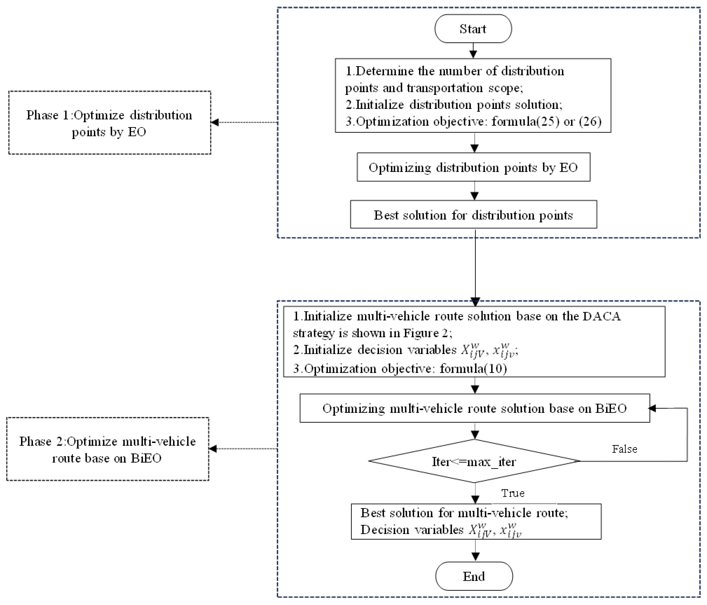
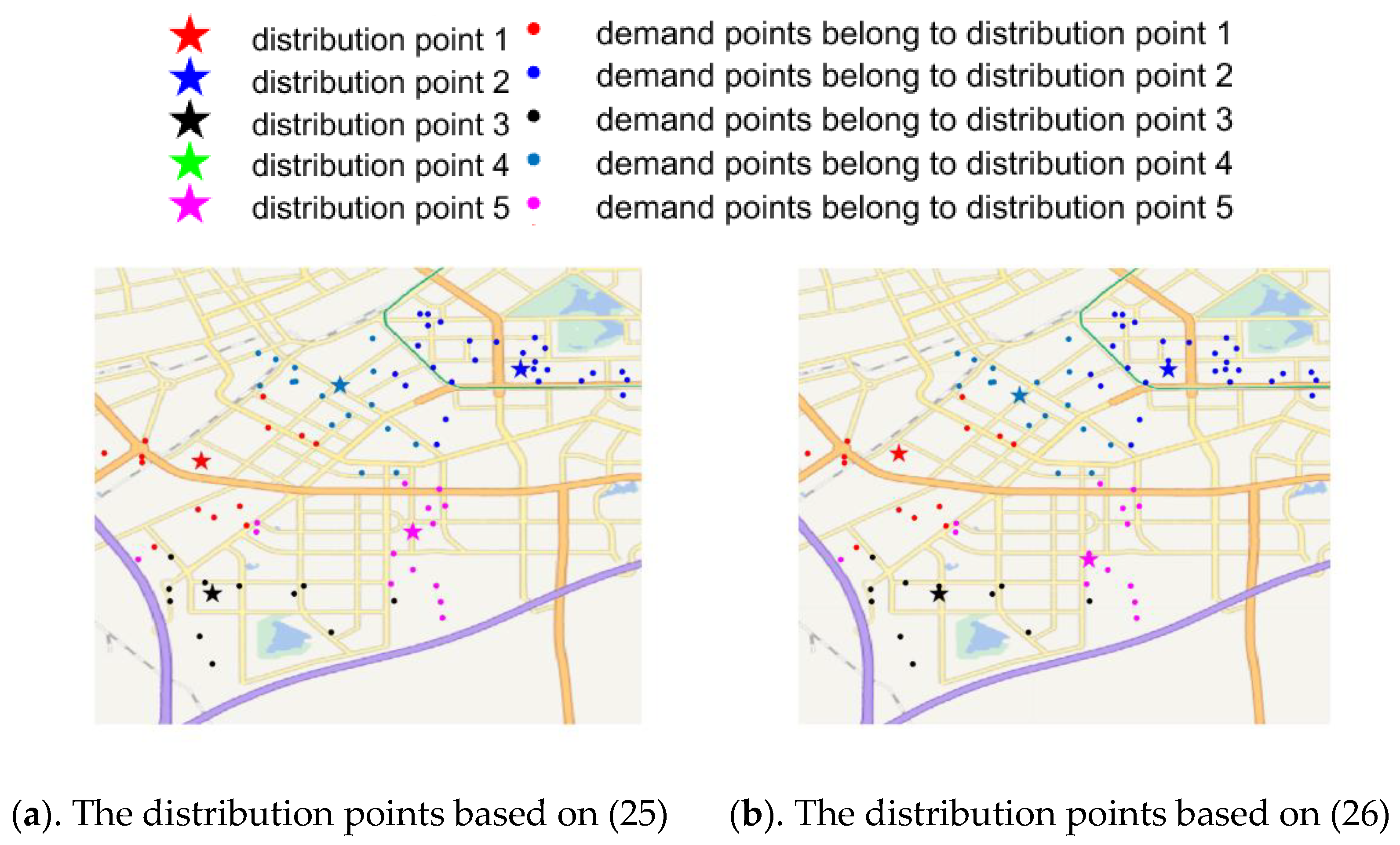
This paper proposed the BiEO algorithm, comprising two main components: (1) addressing the placement of distribution points location problem, Meanwhile, this article has designed two options for the location selection of distribution points, and (2) solving the VRP with capacity constraints for each distribution area, utilizing the DACA strategy in this study. A comparative analysis was conducted against combination-VRP experiments, revealing that the BiEO algorithm yielded superior outcomes within this problem framework compared to GA, DE, and PSO algorithms. Furthermore, the proposed DACA strategy effectively tackled both combinatorial problems and VRP simultaneously.

However, this paper also has some limitations. Firstly, in the optimization model of this article, we assume that each person’s daily material demand is fixed (weighing 400 g per person), which cannot truly reflect each person’s daily material demand. In the future, we may consider defining each person’s daily demand in the form of fuzzy numbers. In addition, due to the use of the DACA strategy in the solution, it is necessary to maintain consistency between the dimensions and the number of demand points in the distribution area during the solving process. Therefore, in this problem, when the transportation vehicle load cannot reach the next demand point in the distribution area, it will return and cannot transport to the demand points in other areas that meet the demand, which may lead to an overall increase in the cost of the problem. In future research, we may consider that transportation vehicles can deliver to demand points outside of this distribution area.

References

1. Salhi, S.; Rand, G.K. The effect of ignoring routes when locating depots. Eur. J. Oper. Res. 1989, 39, 150–156. [Google Scholar] [CrossRef]
2. Hu, H.; Li, X.; Zhang, Y.; Shang, C.; Zhang, S. Multi-objective location-routing model for hazardous material logistics with traffic restriction constraint in inter-city roads. Comput. Ind. Eng. 2019, 128, 861–876. [Google Scholar] [CrossRef]
3. Oksuz, M.K.; Satoglu, S.I. A two-stage stochastic model for location planning of temporary medical centers for disaster response. Int. J. Disaster Risk Reduct. 2020, 44, 101426. [Google Scholar] [CrossRef]
4. Karagöz, S.; Deveci, M.; Simic, V.; Aydin, N. Interval type-2 Fuzzy ARAS method for recycling facility location problems. Appl. Soft Comput. 2021, 102, 107107. [Google Scholar] [CrossRef]
5. Kara, I.; Bektas, T. Integer linear programming formulation of the generalized vehicle routing problem. In Proceedings of the 5-th EURO/INFORMS Joint International Meeting, İstanbul, Turkey, 6–10 July 2003. [Google Scholar]
6. Posada, A.; Rivera, J.C.; Palacio, J.D. A mixed-integer linear programming model for a selective vehicle routing problem. In Proceedings of the Applied Computer Sciences in Engineering: 5th Workshop on Engineering Applications, WEA 2018, Medellín, Colombia, 17–19 October 2018; pp. 108–119. [Google Scholar]
7. Pop, P.C.; Kara, I.; Marc, A.H. New mathematical models of the generalized vehicle routing problem and extensions. Appl. Math. Model. 2012, 36, 97–107. [Google Scholar] [CrossRef]
8. Qin, W.; Zhuang, Z.; Huang, Z.; Huang, H. A novel reinforcement learning-based hyper-heuristic for heterogeneous vehicle routing problem. Comput. Ind. Eng. 2021, 156, 107252. [Google Scholar] [CrossRef]
9. Altabeeb, A.M.; Mohsen, A.M.; Abualigah, L.; Ghallab, A. Solving capacitated vehicle routing problem using cooperative firefly algorithm. Appl. Soft Comput. 2021, 108, 107403. [Google Scholar] [CrossRef]
10. Rabbouch, B.; Saâdaoui, F.; Mraihi, R. Efficient implementation of the genetic algorithm to solve rich vehicle routing problems. Oper. Res. 2021, 21, 1763–1791. [Google Scholar] [CrossRef]
11. Maranzana, F. On the location of supply points to minimize transport costs. J. Oper. Res. Soc. 1964, 15, 261–270. [Google Scholar] [CrossRef]
12. Webb, M. Cost functions in the location of depots for multiple-delivery journeys. J. Oper. Res. Soc. 1968, 19, 311–320. [Google Scholar] [CrossRef]
13. Nagy, G.; Salhi, S. Location-routing: Issues, models and methods. Eur. J. Oper. Res. 2007, 177, 649–672. [Google Scholar] [CrossRef]
14. Muñoz-Villamizar, A.F.; Montoya-Torres, J.R.; Herazo-Padilla, N. Mathematical Programming Modeling and Resolution of the Location-Routing Problem in Urban Logistics. Ing. Y Univ. 2014, 18, 271–289. [Google Scholar] [CrossRef]
15. Heidari, M.; Jafari, M.J.; Rahbari, M. Modeling a Multi-Objective Location-Routing Problem for Hazardous Materials with CO2 Emissions Consideration. In Proceedings of the 14th International Industrial Engineering Conference (IIEC 2018), Tehran, Iran, 7 February 2018. [Google Scholar]
16. Shaerpour, M.; Azani, M.; Aghsami, A.; Rabbani, M. A new fuzzy bi-objective mixed-integer linear programming for designing a medical waste management network in the Coronavirus epidemic: A case study. Int. J. Manag. Sci. Eng. Manag. 2023, 1–16. [Google Scholar] [CrossRef]
17. Cao, J.X.; Wang, X.; Gao, J. A two-echelon location-routing problem for biomass logistics systems. Biosyst. Eng. 2021, 202, 106–118. [Google Scholar] [CrossRef]
18. Biuki, M.; Kazemi, A.; Alinezhad, A. An integrated location-routing-inventory model for sustainable design of a perishable products supply chain network. J. Clean. Prod. 2020, 260, 120842. [Google Scholar] [CrossRef]
19. Ferreira, K.M.; de Queiroz, T.A. A simulated annealing based heuristic for a location-routing problem with two-dimensional loading constraints. Appl. Soft Comput. 2022, 118, 108443. [Google Scholar] [CrossRef]
20. Akpunar, Ö.Ş.; Akpinar, Ş. A hybrid adaptive large neighbourhood search algorithm for the capacitated location routing problem. Expert Syst. Appl. 2021, 168, 114304. [Google Scholar] [CrossRef]
21. Ting, C.-J.; Chen, C.-H. A multiple ant colony optimization algorithm for the capacitated location routing problem. Int. J. Prod. Econ. 2013, 141, 34–44. [Google Scholar] [CrossRef]
22. Vincent, F.Y.; Lin, S.-W.; Lee, W.; Ting, C.-J. A simulated annealing heuristic for the capacitated location routing problem. Comput. Ind. Eng. 2010, 58, 288–299. [Google Scholar]
23. Zhang, H.; Liu, F.; Ma, L.; Zhang, Z. A hybrid heuristic based on a particle swarm algorithm to solve the capacitated location-routing problem with fuzzy demands. IEEE Access 2020, 8, 153671–153691. [Google Scholar] [CrossRef]
24. Peng, Z.; Manier, H.; Manier, M.-A. Particle swarm optimization for capacitated location-routing problem. IFAC-Pap. 2017, 50, 14668–14673. [Google Scholar] [CrossRef]
25. Yu, X.; Zhou, Y.; Liu, X.-F. A novel hybrid genetic algorithm for the location routing problem with tight capacity constraints. Appl. Soft Comput. 2019, 85, 105760. [Google Scholar] [CrossRef]
26. Nguyen, V.-P.; Prins, C.; Prodhon, C. Solving the two-echelon location routing problem by a GRASP reinforced by a learning process and path relinking. Eur. J. Oper. Res. 2012, 216, 113–126. [Google Scholar] [CrossRef]
27. Nguyen, V.-P.; Prins, C.; Prodhon, C. A multi-start iterated local search with tabu list and path relinking for the two-echelon location-routing problem. Eng. Appl. Artif. Intell. 2012, 25, 56–71. [Google Scholar] [CrossRef]
28. Ghaffari-Nasab, N.; Jabalameli, M.S.; Aryanezhad, M.B.; Makui, A. Modeling and solving the bi-objective capacitated location-routing problem with probabilistic travel times. Int. J. Adv. Manuf. Technol. 2013, 67, 2007–2019. [Google Scholar] [CrossRef]
29. Zarandi, M.H.F.; Hemmati, A.; Davari, S. The multi-depot capacitated location-routing problem with fuzzy travel times. Expert Syst. Appl. 2011, 38, 10075–10084. [Google Scholar] [CrossRef]
30. Belenguer, J.-M.; Benavent, E.; Prins, C.; Prodhon, C.; Calvo, R.W. A branch-and-cut method for the capacitated location-routing problem. Comput. Oper. Res. 2011, 38, 931–941. [Google Scholar] [CrossRef]
31. Baldacci, R.; Mingozzi, A.; Wolfler Calvo, R. An exact method for the capacitated location-routing problem. Oper. Res. 2011, 59, 1284–1296. [Google Scholar] [CrossRef]
32. Contardo, C.; Cordeau, J.-F.; Gendron, B. An exact algorithm based on cut-and-column generation for the capacitated location-routing problem. INFORMS J. Comput. 2014, 26, 88–102. [Google Scholar] [CrossRef]
33. Ponboon, S.; Qureshi, A.G.; Taniguchi, E. Branch-and-price algorithm for the location-routing problem with time windows. Transp. Res. Part E Logist. Transp. Rev. 2016, 86, 1–19. [Google Scholar] [CrossRef]
34. Prins, C.; Prodhon, C.; Calvo, R.W. Solving the capacitated location-routing problem by a GRASP complemented by a learning process and a path relinking. 4OR 2006, 4, 221–238. [Google Scholar] [CrossRef]
35. Duhamel, C.; Lacomme, P.; Prins, C.; Prodhon, C. A GRASP× ELS approach for the capacitated location-routing problem. Comput. Oper. Res. 2010, 37, 1912–1923. [Google Scholar] [CrossRef]
36. Jokar, A.; Sahraeian, R. A heuristic based approach to solve a capacitated location-routing problem. J. Mgmt. Sustain. 2012, 2, 219. [Google Scholar] [CrossRef]
37. Lopes, R.B.; Ferreira, C.; Santos, B.S. A simple and effective evolutionary algorithm for the capacitated location–routing problem. Comput. Oper. Res. 2016, 70, 155–162. [Google Scholar] [CrossRef]
38. Quintero-Araujo, C.L.; Caballero-Villalobos, J.P.; Juan, A.A.; Montoya-Torres, J.R. A biased-randomized metaheuristic for the capacitated location routing problem. Int. Trans. Oper. Res. 2017, 24, 1079–1098. [Google Scholar] [CrossRef]
39. Faramarzi, A.; Heidarinejad, M.; Stephens, B.; Mirjalili, S. Equilibrium optimizer: A novel optimization algorithm. Knowl.-Based Syst. 2019, 191, 105190. [Google Scholar] [CrossRef]
40. Ali Shaik, M.; Mareddy, P.L.; Visali, N. Enhancement of Voltage Profile in the Distribution system by Reconfiguring with DG placement using Equilibrium Optimizer. Alex. Eng. J. 2022, 61, 4081–4093. [Google Scholar] [CrossRef]
Figure 1. EO algorithm.
Axioms 13 00031 g001
Figure 2. The DACA strategy for multi-vehicles. (a) Schematic diagram of route coding. (b) Example of DACA strategy initialization.
Axioms 13 00031 g002
Figure 3. The optimization of distribution point location and multi-vehicle route.
Axioms 13 00031 g003
Figure 4. The particle update process of the BiEO algorithm.
Axioms 13 00031 g004aAxioms 13 00031 g004b
Figure 5. The location of distribution points.
Axioms 13 00031 g005
Figure 6. The best solution for vehicle assembly combination and its delivery route. (a). The best multi-vehicle route solution of the No. 3 distribution point. (b). Corresponding vehicle routes in the No. 3 distribution point.
Axioms 13 00031 g006