Weighted Pseudo-θ-Almost Periodic Sequence and Finite-Time Guaranteed Cost Control for Discrete-Space and Discrete-Time Stochastic Genetic Regulatory Networks with Time Delays

Abstract

This paper considers the dual hybrid effects of discrete-time stochastic genetic regulatory networks and discrete-space stochastic genetic regulatory networks in difference formats of exponential Euler difference and second-order central finite difference. The existence of a unique-weight pseudo-$\theta$-almost periodic sequence solution for discrete-time and discrete-space stochastic genetic regulatory networks on the basis of discrete constant variation formulation is discussed, as well as the theory of semi-flow and metric dynamical systems. Furthermore, a finite-time guaranteed cost controller is constructed to reach global exponential stability of these discrete networks via establishing a framework of drive, response, and error networks. The results indicate that spatial diffusions of non-negative dense coefficients have no influence on the global existence of the unique weighted pseudo-$\theta$-almost periodic sequence solution of the networks. The present study is a basic work in the consideration of discrete spatial diffusion in stochastic genetic regulatory networks and serves as a foundation for further study.

1. Introduction

Genetic regulatory networks (GRNs) have been widely recognized due to their possible usages [1]. GRNs are actually a complex dynamical system that describes the regulatory mechanisms of DNA, mRNA, and protein interactions in biological systems at the molecular level [2,3]. The analysis of genetic regulatory networks is not only an important way to understand and grasp the operation mechanisms of the activity of cellular life [4], but also has promising applications in the fields of disease genetic prediction and drug target screening [5,6,7,8]. For this reason, it is necessary and valuable to propose suitable mathematical models to represent expression mechanisms and signal transduction pathways. Currently, GRNs are generally modeled by Boolean models, Bayesian models, and differential equation models. Two of the most widely used models are Boolean models and differential equation models [9,10,11]. In particular, differential equations describe the concentration changes in proteins and mRNA [12,13]. This model has received more attention because of its higher accuracy and its ability to accurately describe the nonlinear dynamic behaviour of biological systems.

In general, the majority of models utilised to characterize GRNs in the currently available literature suppose that the concentrations of mRNAs and proteins are spatially homogeneous at all times. However, this assumption has some limitations, for example the diffusion phenomenon should be considered for the case of non-uniform distributions of gene product concentrations [14]. Therefore, the issue of kinetic analysis of GRNs with reaction–diffusion effects is worth investigating. Moreover, time delay is often inevitable due to the finite processing time of interactions among agents and may influence system performance. As of recently, a great deal of results on GRNs with time delays can be found in the literature, see, e.g., Han et al. [14], who established an asymptotic stability criterion for reaction–diffusion delayed GRNs under Dirichlet and Neumann boundary conditions, respectively, insightfully recognizing that diffusion–reaction information can reduce the conservation of the system. Robust state estimation of delayed genetic regulatory networks with reaction–diffusion terms and uncertainty terms under the Dirichlet boundary condition is considered by Zou et al. in [15]. Xie et al. [16] discuss the stability of genetic regulatory networks, centralised spatial diffusion, and discrete and infinite distribution delays.

During the processes of both computational simulation and analysis, engineers often use discrete-time continuous models to evaluate their structural behaviour. The signals received and operated in digital networks are dependent on discrete-time rather than continuous-time. Therefore, discrete-time GRNs have been studied by many authors. For example, Xue et al. [17] investigate the problems of state boundary description and reachable set estimation for discrete-time delayed genetic regulatory networks with bounded perturbations. Liu et al. [18] study the problem of exponential stability analysis of discrete genetic regulatory networks with time-varying discrete-time delays and unbounded distributed time delays. Yue et al. [19] investigate the dynamics of discrete-time genetic models and obtain conditions for the existence and stability of fixed points. It is shown that the discrete-time genetic network undergoes fold bifurcation, flip bifurcation, and Neimark–Sacker bifurcation, illuminating the richer dynamical properties of the discrete-time genetic model than the original continuous-time model. It is worth noting that most of the results on GRNs only concern discrete-time GRNs [17,18,19,20,21,22], while the results on spatial discrete GRNs have not received sufficient attention in existing studies, probably owing to the partial ineffectiveness of traditional methods in space–time continuous networks, such as the Lyapunov–Krasovskii general functions in discrete-space and -time networks, and the difficulty of computing the difference. To date, there are several reports referring to space–time discrete models [23,24,25]; nevertheless, the models of stochastic space–time discrete GRNs have not been deeply addressed.

It is well known that stochastic uncertainty is inevitable in various dynamical systems, with reference to its ability to alter the mechanical properties of genetic regulatory networks in practical applications. Therefore, the dynamic behaviour of delayed stochastic genetic regulatory networks has been extensively studied, see the literature [26,27,28,29]. For example, Xu et al. [26] investigate the input state stability problem of stochastic gene regulation networks with multiple time delays, and give sufficient conditions for the mean square exponential input state stability of the system using the Lyapunov generalization, Ito’s formula, and Dynkin’s formula. Wang [29] investigates the dual effects of discrete space and discrete time in stochastic genetic regulatory networks by means of exponential Eulerian differences and central finite differences. In addition, finite-time guaranteed cost control is a very effective method in the engineering field due to its many advantages in practical applications, see references [30,31,32,33,34,35,36,37]. The advantages of finite-time guaranteed cost controllers are listed below: (1) Stability. A finite-time guaranteed cost controller is a feedback controller that adjusts the system to remain stable when it is subject to external disturbances or internal changes. (2) Reliability. It can adjust the control strategy adaptively depending on the state of the system, so as to increase the reliability of the system. In summary, the finite-time cost-preserving controller is an advanced control method for genetic regulatory networks with many advantages that can assist the system to be more stable, reliable, and robust, and optimise the performance index of the system.

On the other hand, the global exponential stability and almost periodic nature of GRNs are significant and necessary dynamical behaviours that have been extensively researched by many authors in the last two decades, see the literature [18,38,39,40,41,42]. Particularly in stochastic models, the notion of $\theta$-almost periodicity was first introduced in the paper [43] on the basis of semi-flow and metric dynamical system theories, and the existence of $\theta$-almost periodicity for several continuous-time stochastic models was investigated [44,45]. First, pseudo-almost periodicity was introduced in the early 1990s by Zhang [46] as a natural extension of classical probability periodicity. Since then, pseudo-approximate periodic solutions of differential equations have attracted a lot of attention. In the literature [47], Diagana extended pseudo-almost periodicity to weighted pseudo-almost periodicity and reported a number of excellent contributions on weighted pseudo-almost periodicity, see references [48,49,50]. However, the study of the $\theta$-almost periodicity of stochastic discrete-time GRNs, not to mention weighted pseudo-$\theta$-almost periodicity, influenced by spatial diffusion, has not been addressed in depth so far.

Based on the above motivation, the main purpose of this paper is to establish discrete-time stochastic genetic regulatory networks (SGRNs) for discrete-space diffusion using exponential Euler difference and central finite difference methods. On this ground, a discrete constant variation formula for discrete SGRNs is derived. On the basis of the discrete constant variation formula, the weighted pseudo-$\theta$-almost periodicity of discrete SGRNs with discrete spatial diffusion is investigated by combining the theory of semi-fluid dynamical systems and metric dynamical systems. In the end, a finite-time guaranteed cost controller for this type of SGRN is designed by the construction of a drive, response, and error network framework. The main studies and innovations of this paper are briefly summarised in turn as follows.

(1)

Discrete-time and discrete-space SGRNs are newly introduced, which extends the studied models in reports [18,40].

(2)

The weighted pseudo-$\theta$-almost periodicity of this class of SGRNs is considered for the first time, which complements the works on the almost periodicity of GRNs in references [12,38].

(3)

Finite-time cost-preserving controllers are designed for this class of SGRNs.

Plan of this paper: In Section 2, a formula for discrete-time and discrete-space SGRNs is given and the concept of weighted pseudo-$\theta$-almost periodicity is presented. Section 3 discusses the global existence of unique weighted pseudo-$\theta$-almost periodic sequence solutions for discrete-time and discrete-space SGRNs on the basis of the theory of semifluid and metric dynamical systems, the discrete constant variation formula, and the fixed-point theorem. Furthermore, in Section 4, finite-time cost-preserving controllers are designed by constructing a framework of drive, response, and error networks for discrete-time and discrete-space SGRNs. Section 5 gives numerical examples of discrete-time and discrete-space SGRNs achieving weight pseudo-$\theta$-almost periodicity, finite-time guaranteed cost control, and global exponential stability. The conclusions and main points of the paper are given in Section 6.

Symbols: ${\mathbb{R}}^n$ denotes the space of n-dimensional real vectors; $\mathbb{Z}$ is the field of integral numbers; ${\mathbb{N}}_0=\{0,1,2,\dots \}$; $\mathbb{N}={\mathbb{N}}_0\setminus \left\{0\right\}$; ${\mathbb{N}}_a^b=\{a,a+1,\dots ,b\}$ for any $a,b\in \mathbb{Z}$; $I_J=I\cap J$, $\forall I,J\subseteq \mathbb{R}$. Let ${\xi }_1={(1,0,\dots ,0)}^T,$ ${\xi }_2={(0,1,\dots ,0)}^T,\dots$ ${\xi }_m={(0,0,\dots ,1)}^T$.

Define $N_p\in \mathbb{N}$ for $p\in {\mathbb{N}}_1^m$, ${\mho }_{\nu }:=\left\{\nu ={({\nu }_1,\dots ,{\nu }_m)}^T:({\nu }_p,p)\in ({\mathbb{N}}_1^{N_p-1},{\mathbb{N}}_1^m)\right\}$, $\partial {\mho }_{\nu }:={\overline{\mho }}_{\nu }\setminus {\mho }_{\nu }$, ${\overline{\mho }}_{\nu }=\left\{\nu ={({\nu }_1,\dots ,{\nu }_m)}^T:({\nu }_p,p)\in ({\mathbb{N}}_0^{N_p},{\mathbb{N}}_1^m)\right\}.$

For any function $f:{\overline{\mho }}_{\nu }\times \mathbb{Z}$ to ${\mathbb{R}}^n$, we denote as $f:=f_k^{\langle \nu \rangle }={(f_{1,k}^{\langle \nu \rangle },\dots ,f_{n,k}^{\langle \nu \rangle })}^T$, where $(\nu ,k)\in {\overline{\mho }}_{\nu }\times \mathbb{Z}$. Sometimes, $f={(f_1,\dots ,f_n)}^T$ is used for simplicity.

2. Problem Formulation

In this section, firstly, discrete-time and discrete-space SGRNs are presented, which can be considered as discrete formats of continuous-time SGRNs with reaction diffusion. Secondly, the constant variation formula of the discrete network is obtained by dividing the discrete network into two discrete sub-networks based on the theory of difference equations. In the next step, important inequalities are given, such as the Minkowski inequality in Lemma 2. Finally, the definition of weighted pseudo-$\theta$-almost periodicity is presented.

2.1. Space–Time Discrete Stochastic GRNs

This article considers the following space–time discrete stochastic genetic regulatory networks (GRNs) in the Euler form of

$$\left\{\begin{array}{ccc}{\displaystyle {\mathbf{m}}_{i,k+1}^{\langle \nu \rangle }}\hfill & =\hfill & {\displaystyle e^{-a_{i,k}h}{\mathbf{m}}_{i,k}^{\langle \nu \rangle }+\frac{1-e^{-a_{i,k}h}}{a_{i,k}}[\sum _{q=1}^n{\mathsf{\Theta }}_{iq}{\tilde{\Delta }}_{{\hslash }_q}^2{\mathbf{m}}_{i,k}^{\langle \nu \rangle }}\hfill \\ \hfill & \hfill & {\displaystyle +\sum _{j=1}^m{b}_{ij,k}{f}_j\left({\mathbf{p}}_{j,k-{\sigma }_{j,k}}^{\langle \nu \rangle }\right)+\sum _{j=1}^m{\gamma }_{ij,k}{g}_j\left({\mathbf{p}}_{j,k-{\mu }_{j,k}}^{\langle \nu \rangle }\right)w_{1j,k}+I_{i,k}],}\hfill \\ {\mathbf{p}}_{i,k+1}^{\langle \nu \rangle }\hfill & =\hfill & {\displaystyle e^{-c_{i,k}h}{\mathbf{p}}_{i,k}^{\langle \nu \rangle }+\frac{1-e^{-c_{i,k}h}}{c_{i,k}}\left[\sum _{q=1}^n{\Pi }_{iq}{\tilde{\Delta }}_{{\hslash }_q}^2{\mathbf{p}}_{i,k}^{\langle \nu \rangle }+d_{i,k}{\mathbf{m}}_{i,k}^{\langle \nu \rangle }+\sum _{j=1}^m{\varpi }_{ij,k}{\eta }_j\left({\mathbf{m}}_{j,k-{\nu }_{j,k}}^{\langle \nu \rangle }\right)w_{2j,k}\right]}\hfill \end{array}\right.$$

(1)

for $(\nu ,k)\in {\mho }_{\nu }\times \mathbb{Z}$ and $i=1,2,\dots ,m$; ${\mathbf{m}}_i$ and ${\mathbf{p}}_i$ denote the concentrations of the ith mRNA and ith protein, respectively;

$${\tilde{a}}_i=a_i-2\sum _{q=1}^n\frac{{\mathsf{\Theta }}_{iq}}{{\hslash }^2},{\tilde{c}}_i=c_i-2\sum _{q=1}^n\frac{{\Pi }_{iq}}{{\hslash }^2},$$

${\tilde{a}}_i>0$ and ${\tilde{c}}_i>0$ are the decay rates of the ith mRNA and ith protein, respectively; ${\mathsf{\Theta }}_{iq}$ and ${\Pi }_{iq}$ represent the transmission diffusion matrixes, where ${\tilde{\Delta }}_{{\hslash }_q}^2$ means the discrete-space operator denoted by

$${\tilde{\Delta }}_{{\hslash }_q}^2{\mathbf{m}}_{i,·}^{\langle ·\rangle }:=\frac{{\mathbf{m}}_{i,·}^{\langle \nu +{\xi }_q\rangle }+{\mathbf{m}}_{i,·}^{\langle \nu -{\xi }_q\rangle }}{{\hslash }^2},{\tilde{\Delta }}_{{\hslash }_q}^2{\mathbf{p}}_{i,·}^{\langle ·\rangle }:=\frac{{\mathbf{p}}_{i,·}^{\langle \nu +{\xi }_q\rangle }+{\mathbf{p}}_{i,·}^{\langle \nu -{\xi }_q\rangle }}{{\hslash }^2},q\in {\mathbb{N}}_1^n;$$

ℏ and h denote the length of the space and time steps in order; ${\gamma }_{ij}$ and ${\varpi }_{ij}$ stand for noise intensities; $d_i>0$ is the translation rate; $I_i={\sum }_{j\in {\mathbf{I}}_i}{w}_{ij},w_{ij}\ge 0$ is bounded and ${\mathbf{I}}_i$ is the set of all the j which is a repressor of gene i; $b_{ij}=w_{ij}$ if transcription factor j is an activator of gene i, $b_{ij}=0$ if there is no link from node j to i, and $b_{ij}=-w_{ij}$ if transcription factor j is a repressor of gene i; $f_j$, $g_j$, and ${\eta }_j$ are Hill functions; $w_{1j,k}:=\frac{1}{h}[{\mathbf{w}}_{1j}(kh+h)-{\mathbf{w}}_{1j}\left(kh\right)]$, $w_{2j,k}:=\frac{1}{h}[{\mathbf{w}}_{2j}(kh+h)-{\mathbf{w}}_{2j}\left(kh\right)]$, and $i,j=1,2,\dots ,m$; ${\mathbf{w}}_{11},\dots ,{\mathbf{w}}_{1m},{\mathbf{w}}_{21},\dots ,{\mathbf{w}}_{2m}$ are scalar mutually independent two-sided standard Brown motions on complete probability space $(\mathsf{\Omega },\mathcal{F},{\mathcal{F}}_{·},\mathbf{P})$ with filtration

$${\mathcal{F}}_k=\sigma \left\{(w_{11,q},\dots ,w_{1m,q},w_{21,q},\dots ,w_{2m,q}):q\in {(-\infty ,k)}_{\mathbb{Z}}\right\},\forall k\in \mathbb{Z}.$$

The Dirichlet boundary conditions of GRNs Equation (1) are described as

$${\mathbf{m}}_{i,k}^{\langle \nu \rangle }{|}_{\nu \in \partial {\mho }_{\nu }}=0={\mathbf{p}}_{i,k}^{\langle \nu \rangle }{|}_{\nu \in \partial {\mho }_{\nu }},\forall k\in \mathbb{Z}.$$

(2)

Herein, ${\mho }_{\nu }$ can be regarded as a discrete form of the rectangle area ℧ in ${\mathbb{R}}^m$, which is described by

$$\mho =\left\{x={(x_1,x_2,\dots ,x_m)}^T\in {\mathbb{R}}^m:0<x_p<L_p:=\hslash N_p,p\in {\mathbb{N}}_1^m\right\}.$$

Let ${\mathbf{m}}_{i,k}^{\langle \nu \rangle }=M_i(\nu \hslash ,kh)$ and ${\mathbf{p}}_{i,k}^{\langle \nu \rangle }=P_i(\nu \hslash ,kh)$ for $(\nu ,k)\in {\mho }_{\nu }\times \mathbb{Z}$. Then, GRNs Equation (1) is a full discretization scheme of the following stochastic GRNs with reaction diffusions

$$\begin{array}{c}\hfill \left\{\begin{array}{c}{\displaystyle \frac{\partial }{\partial t}{M}_i(x,t)=\sum _{q=1}^n\frac{\partial }{\partial x_q}\left[{\mathsf{\Theta }}_{iq}\frac{\partial M_i(x,t)}{\partial x_q}\right]-{\tilde{a}}_i\left(t\right)M_i(x,t)}\hfill \\ {\displaystyle +\sum _{j=1}^m{b}_{ij}\left(t\right)f_j\left(P_j(x,t-{\sigma }_j\left(t\right))\right)+I_i\left(t\right)+\sum _{j=1}^m{\gamma }_{ij}(x,t)g_j\left(P_j(x,t-{\mu }_j\left(t\right))\right)\frac{\mathrm{d}}{\mathrm{d}t}{\mathbb{W}}_{1j}\left(t\right),}\hfill \\ {\displaystyle \frac{\partial }{\partial t}{P}_i(x,t)=\sum _{q=1}^n\frac{\partial }{\partial x_q}\left[{\Pi }_{iq}\frac{\partial P_i(x,t)}{\partial x_q}\right]-{\tilde{c}}_i\left(t\right)P_i(x,t)}\hfill \\ {\displaystyle +d_i(x,t)M_i(x,t)+\sum _{j=1}^m{\varpi }_{ij}(x,t){\eta }_j\left(M_j(x,t-{\nu }_j\left(t\right))\right)\frac{\mathrm{d}}{\mathrm{d}t}{\mathbb{W}}_{2j}\left(t\right),}\hfill \\ M_i(x,t){|}_{x\in \partial \mho }=0=P_i(x,t){|}_{x\in \partial \mho },\hfill \end{array}\right.\end{array}$$

(3)

where $x={(x_1,\dots ,x_n)}^T\in \mho \subseteq {\mathbb{R}}^n$ refers to a space variable.

The discrete techniques in SGRNs Equation (1) are therefore Eulerian difference (ED) for Brownian motion, exponential Eulerian difference (EED) for time variables, and central finite difference (CFD) for spatial variables, respectively. For more information on ED, EED, and CFD, please see the literature [51,52,53,54,55].

Remark 1.

By using Euler differences, reports [18,40] considered discrete-time GRNs without spatial diffusions. In this article, SGRNs Equation (1) extends the models in reports [18,40].

Lemma 1.

GRNs Equation (1) can be expressed as

$$\left\{\begin{array}{ccc}{\displaystyle {\mathbf{m}}_{i,k}^{\langle \nu \rangle }}\hfill & =\hfill & {\displaystyle \prod _{s=k_0}^{k-1}{e}^{-a_{i,s}h}{\mathbf{m}}_{i,k_0}^{\langle \nu \rangle }+\sum _{v=k_0}^{k-1}\prod _{s=v+1}^{k-1}\frac{e^{-a_{i,s}h}(1-e^{-a_{i,v}h})}{a_{i,v}}}\hfill \\ & \hfill & {\displaystyle \times \left[\sum _{q=1}^n{\mathsf{\Theta }}_{iq}{\tilde{\Delta }}_{{\hslash }_q}^2{\mathbf{m}}_{i,v}^{\langle \nu \rangle }+\sum _{j=1}^m{b}_{ij,v}{f}_j\left({\mathbf{p}}_{j,v-{\sigma }_{j,v}}^{\langle \nu \rangle }\right)+\sum _{j=1}^m{\gamma }_{ij,v}{g}_j\left({\mathbf{p}}_{j,v-{\mu }_{j,v}}^{\langle \nu \rangle }\right)w_{1j,v}+I_{i,v}\right],}\hfill \\ {\mathbf{p}}_{i,k}^{\langle \nu \rangle }\hfill & =\hfill & {\displaystyle \prod _{s=k_0}^{k-1}{e}^{-c_{i,s}h}{\mathbf{p}}_{i,k_0}^{\langle \nu \rangle }+\sum _{v=k_0}^{k-1}\prod _{s=v+1}^{k-1}\frac{e^{-c_{i,s}h}(1-e^{-c_{i,v}h})}{c_{i,v}}}\hfill \\ & \hfill & {\displaystyle \times \left[\sum _{q=1}^n{\Pi }_{iq}{\tilde{\Delta }}_{{\hslash }_q}^2{\mathbf{p}}_{i,v}^{\langle \nu \rangle }+d_{i,v}{\mathbf{m}}_{i,v}^{\langle \nu \rangle }+\sum _{j=1}^m{\varpi }_{ij,v}{\eta }_j\left({\mathbf{m}}_{j,v-{\nu }_{j,v}}^{\langle \nu \rangle }\right)w_{2j,v}\right],}\hfill \end{array}\right.$$

(4)

where $(\nu ,k)\in {\mho }_{\nu }\times {[k_0,\infty )}_{\mathbb{Z}}$ with some initial point $k_0\in \mathbb{Z}$, $i=1,2,\dots ,m$. Moreover, it holds that

$${\mathbf{m}}_{i,k}^{\langle \nu \rangle }{|}_{\nu \in \partial {\mho }_{\nu }}=0={\mathbf{p}}_{i,k}^{\langle \nu \rangle }{|}_{\nu \in \partial {\mho }_{\nu }},\forall k\in {[k_0,\infty )}_{\mathbb{Z}},i=1,2,\dots ,m.$$

Lemma 2

([56] (Minkowski inequality)). If $X,Y\in L^2(\mathsf{\Omega },\mathbb{R})$, then

$${\left({\mathbf{E}|X+Y|}^2\right)}^{\frac{1}{2}}\le {\left({\mathbf{E}\left|X\right|}^2\right)}^{\frac{1}{2}}+{\left({\mathbf{E}\left|Y\right|}^2\right)}^{\frac{1}{2}}.$$

Lemma 3

([56] $\left(\mathrm{H}\ddot{\mathrm{o}}\mathrm{lder}\mathrm{inequality}\right)$). Let $a_k,b_k:\mathbb{Z}\to \mathbb{R}$. Then,

$$|\sum _k{a}_k{b}_k{|}^2\le \sum _k|a_k|\sum _k|a_k\left|\right|b_k{|}^2.$$

Lemma 4.

$\mathbf{E}|w_{1j,k}{|}^2=\mathbf{E}{\left|w_{2j,k}\right|}^2=\frac{1}{h}$ for $j=1,2,\dots ,n$.

Proof 

By the definition of $w_{1j,k}$ and Ito formula, it is derived that

$$\mathbf{E}|w_{1j,k}{|}^2=\frac{1}{h^2}\mathbf{E}{\left({\int }_{kh}^{kh+h}\mathrm{d}{\mathbb{W}}_{1j}\left(s\right)\right)}^2=\frac{1}{h^2}\mathbf{E}{\int }_{kh}^{kh+h}\mathrm{d}s=\frac{1}{h},\forall j=1,2,\dots ,n.$$

This completes the proof. □

2.2. Weighted Pseudo-Almost Periodicity

In the following, assume that $(\mathbb{X},\parallel ·{\parallel }_{\mathbb{X}})$ is a norm linear space, and $L^p(\mathsf{\Omega },{\mathbb{R}}^n)$ denotes the set of all pth integrable ${\mathbb{R}}^n$-valued random variables with the norm

$${∥u∥}_p=\underset{1\le i\le n}{max}{\left[\mathbf{E}|u_i{|}^p\right]}^{1/p},\forall u={(u_1,\dots ,u_n)}^T\in L^p(\mathsf{\Omega },{\mathbb{R}}^n),p>0,$$

in which $\mathbf{E}$ denotes the expectation operator with respect to probability space $(\mathsf{\Omega },\mathcal{F},\mathbf{P})$.

Definition 1.

Let $X\in \mathbb{X}$ and $ϵ>0$ be arbitrary. If $\nu ={\nu }_{ϵ}$ and $\tau \in {[a,a+{\nu }_{ϵ}]}_{\mathbb{Z}}$ for any $a\in \mathbb{Z}$, ensuring that

$${∥X_{k+\tau }-X_k∥}_{\mathbb{X}}<ϵ,\forall k\in \mathbb{Z},$$

then $\left\{X_k\right\}$ is an almost periodic sequence. Herein, τ is called an ϵ-almost period of X. $AP(\mathbb{Z},\mathbb{X})$ denotes the set of the whole almost periodic sequences.

Let $\mathbb{U}$ be the set of all weight sequences $\alpha :\mathbb{Z}\to (0,+\infty )$ satisfying

$$\frac{{\alpha }_{k+s}}{{\alpha }_k}\le \overline{\alpha },\forall k\in \mathbb{Z},s\in {[0,{\sigma }_0]}_{\mathbb{Z}};$$

$${\mu }_k\left(\alpha \right):=\sum _{s=-k}^k{\alpha }_s\to +\infty ,\frac{1}{{\mu }_k\left(\alpha \right)}\sum _{s=-k-{\sigma }_0}^{-k}{\alpha }_s\to 0,\mathrm{as}k\to +\infty ,$$

where ${\sigma }_0={max}_{1\le j\le m}{sup}_{k\in \mathbb{Z}}\{{\sigma }_{j,k},{\mu }_{j,k},{\nu }_{j,k}\}$.

Define $\mathbb{B}(\mathbb{Z},\mathbb{X})$ as the set of all bounded sequences from $\mathbb{Z}$ to $\mathbb{X}$ and

$$PA{P}_0^{\mu }(\mathbb{Z},\mathbb{X},\alpha ):=\left\{{\displaystyle X\in \mathbb{B}(\mathbb{Z},\mathbb{X}):\underset{k\to +\infty }{lim}\frac{1}{{\mu }_k\left(\alpha \right)}\sum _{s=-k}^k{\alpha }_s{\parallel X_s\parallel }_{\mathbb{X}}=0}\right\}.$$

When $\mathbb{X}=L^2(\mathsf{\Omega },{\mathbb{R}}^n)$ or ${\mathbb{R}}^n$, we use $PA{P}_0^{\mu }(\mathbb{Z},{\mathbb{R}}^n,\alpha )$ to denote $PA{P}_0^{\mu }(\mathbb{Z},\mathbb{X},\alpha )$.

Definition 2.

Sequence $X\in \mathbb{B}(\mathbb{Z},\mathbb{X})$ is said to be a weighted pseudo-almost periodic sequence or an α-pseudo-almost periodic sequence in the case $X=Y+Z$, where $Y\in AP(\mathbb{Z},\mathbb{X})$, $Z\in PA{P}_0^{\mu }(\mathbb{Z},\mathbb{X},\alpha )$, and $\alpha \in \mathbb{U}$. The space of all α-pseudo-almost periodic sequences is represented by $PA{P}^{\mu }(\mathbb{Z},\mathbb{X},\alpha )$.

Supposing that $(\mathsf{\Omega },\mathcal{F},\mathbf{P},\theta )$ is a metric dynamical system, see the pioneering work in [57]. It holds that ${\theta }_k:\mathsf{\Omega }\to \mathsf{\Omega }$ is $\mathcal{F}$-measurable, $\mathbf{P}\left({\theta }_k^{-1}\left(A\right)\right)=\mathbf{P}\left(A\right)$ for any $A\in \mathcal{F}$, and ${\theta }_{s+k}={\theta }_s\circ {\theta }_k$, $\forall s,k\in \mathbb{Z}$.

Definition 3.

The translation to a sequential process $X_k$ is defined as

$${\mathcal{L}}_{\tau }{X}_k\left(\omega \right):=X_{k+\tau }\left({\theta }_{-\tau }\omega \right),\forall \omega \in \mathsf{\Omega },s,k,\tau \in \mathbb{Z}.$$

Definition 4.

If $X_k\in \mathbb{X}$, $\forall k\in \mathbb{Z}$, then X is said to be θ-almost periodic in the case that for each $ϵ>0$ we can find at least one positive integer $\nu =\nu \left(ϵ\right)$ and it has a constant $\tau =\tau \left(ϵ\right)\in {(a,a+\nu )}_{\mathbb{Z}}$ for arbitrary $a\in \mathbb{Z}$, ensuring that

$${∥{\mathcal{L}}_{\tau }{X}_k-X_k∥}_{\mathbb{X}}\le ϵ,\forall k\in \mathbb{Z}.$$

Herein, τ is called an ϵ-θ-almost period of X. The space of all θ-almost periodic sequences is represented by $A{P}^{\theta }(\mathbb{Z},\mathbb{X})$. If ${\mathcal{L}}_{\tau }X=X$ with $\tau \in \mathbb{Z}$, then X is said to be θ-periodic.

When $\mathbb{X}=L^p(\mathsf{\Omega },{\mathbb{R}}^n)$ with $p>0$, then X is said to be θ-almost periodic in p-mean. If $p=2$, the elements in $PA{P}^{\theta }(\mathbb{Z},L^p(\mathsf{\Omega },{\mathbb{R}}^n))$ are called a mean square θ-almost periodic sequence. Hereby, we use a simplified symbol $PA{P}^{\theta }(\mathbb{Z},{\mathbb{R}}^n)$ to denote $PA{P}^{\theta }(\mathbb{Z},L^2(\mathsf{\Omega },{\mathbb{R}}^n))$.

Definition 5.

Sequence $X:\mathbb{Z}\to \mathbb{X}$ is said to be a weighted pseudo-θ-almost periodic sequence or α-pseudo-θ-almost periodic sequence in the case $X=Y+Z$, where $Y\in A{P}^{\theta }(\mathbb{Z},\mathbb{X})$, $Z\in PA{P}_0^{\mu }(\mathbb{Z},\mathbb{X},\alpha )$, and $\alpha \in \mathbb{U}$. The space of all α-pseudo-θ-almost periodic sequences is represented by $PA{P}^{\theta ,\mu }(\mathbb{Z},\mathbb{X},\alpha )$. If Y is θ-periodic, then X is said to be a weighted pseudo-θ-periodic sequence or an α-pseudo-θ-periodic sequence.

When $\mathbb{X}=L^p(\mathsf{\Omega },{\mathbb{R}}^n)$ with $p>0$, then X is said to be a weighted pseudo-θ-almost periodic sequence or an α-pseudo-θ-almost periodic sequence in p-mean. If $p=2$, the elements in $PA{P}^{\theta ,\mu }(\mathbb{Z},L^p(\mathsf{\Omega },{\mathbb{R}}^n),\alpha )$ are called a weighted pseudo mean square θ-almost periodic sequence or an α-pseudo mean square θ-almost periodic sequence. Hereby, a simplified symbol $PA{P}^{\theta ,\mu }(\mathbb{Z},{\mathbb{R}}^n,\alpha ):=PA{P}^{\theta ,\mu }(\mathbb{Z},L^2(\mathsf{\Omega },{\mathbb{R}}^n),\alpha )$.

3. Mean Square $\alpha$-Pseudo-$\theta$-Almost Periodic Sequence

This section focuses on weighted pseudo-$\theta$-almost periodic sequence solutions in the mean square sense of SGRNs Equation (1) based on stochastic calculus theory, the constant variation formula, and the Banach contraction mapping principle.

For any $\mathbf{u}={(\mathbf{m},\mathbf{p})}^T\in PA{P}^{\theta ,\mu }({\mho }_{\nu }\times \mathbb{Z},{\mathbb{R}}^{2m},\alpha )$ with $\mathbf{m}={({\mathbf{m}}_1,\cdots ,{\mathbf{m}}_m)}^T$ and $\mathbf{p}={({\mathbf{p}}_1,\cdots ,{\mathbf{p}}_m)}^T$, define $\Gamma :PA{P}^{\theta ,\mu }({\mho }_{\nu }\times \mathbb{Z},{\mathbb{R}}^{2m},\alpha )\to {\mathbb{R}}^{2m}$ by

$$\Gamma \mathbf{u}={\left((\Phi {\mathbf{u}}_1),\cdots ,{(\Phi \mathbf{u})}_m,{(\Psi \mathbf{u})}_1,\cdots ,{(\Psi \mathbf{u})}_m\right)}^T,$$

where

$$\left\{\begin{array}{ccc}{\displaystyle {(\Phi \mathbf{u})}_{i,k}^{\langle \nu \rangle }}\hfill & =\hfill & {\displaystyle \sum _{v=-\infty }^{k-1}\prod _{s=v+1}^{k-1}\frac{e^{-a_{i,s}h}(1-e^{-a_{i,v}h})}{a_{i,v}}[\sum _{q=1}^n{\mathsf{\Theta }}_{iq}{\tilde{\Delta }}_{{\hslash }_q}^2{\mathbf{m}}_{i,v}^{\langle \nu \rangle }}\hfill \\ & \hfill & {\displaystyle +\sum _{j=1}^m{b}_{ij,v}{f}_j\left({\mathbf{p}}_{j,v-{\sigma }_{j,v}}^{\langle \nu \rangle }\right)+\sum _{j=1}^m{\gamma }_{ij,v}{g}_j\left({\mathbf{p}}_{j,v-{\mu }_{j,v}}^{\langle \nu \rangle }\right)w_{1j,v}+I_{i,v}],}\hfill \\ {(\Psi \mathbf{u})}_{i,k}^{\langle \nu \rangle }\hfill & =\hfill & {\displaystyle \sum _{v=-\infty }^{k-1}\prod _{s=v+1}^{k-1}\frac{e^{-c_{i,s}h}(1-e^{-c_{i,v}h})}{c_{i,v}}[\sum _{q=1}^n{\Pi }_{iq}{\tilde{\Delta }}_{{\hslash }_q}^2{\mathbf{p}}_{i,v}^{\langle \nu \rangle }}\hfill \\ & \hfill & {\displaystyle +\sum _{j=1}^m{\varpi }_{ij,v}{\eta }_j\left({\mathbf{m}}_{j,v-{\nu }_{j,v}}^{\langle \nu \rangle }\right)w_{2j,v}+d_{i,v}{\mathbf{m}}_{i,v}^{\langle \nu \rangle }],\forall (\nu ,k)\in {\mho }_{\nu }\times \mathbb{Z};}\hfill \end{array}\right.$$

(5)

${(\Phi \mathbf{u})}_{i,k}^{\langle \nu \rangle }{|}_{\nu \in \partial {\mho }_{\nu }}=0={(\Psi \mathbf{u})}_{i,k}^{\langle \nu \rangle }{|}_{\nu \in \partial {\mho }_{\nu }}$, $\forall k\in \mathbb{Z}$, $i=1,2,\dots ,m.$

For $\forall \mathbf{u}=(\mathbf{m},\mathbf{p})\in PA{P}^{\theta ,\mu }({\mho }_{\nu }\times \mathbb{Z},{\mathbb{R}}^{2m},\alpha )$, define the norm as follows:

$${\parallel \mathbf{u}\parallel }_{\infty }=\underset{(\nu ,k)\in {\mho }_{\nu }\times \mathbb{Z}}{sup}\underset{1\le i\le m}{max}\left\{{∥{\mathbf{m}}_{i,k}^{\langle \nu \rangle }∥}_2,{∥{\mathbf{p}}_{i,k}^{\langle \nu \rangle }∥}_2\right\},$$

in which ${∥{\mathbf{m}}_{i,k}^{\langle \nu \rangle }∥}_2={\left[\mathbf{E}{\left({\mathbf{m}}_{i,k}^{\langle \nu \rangle }\right)}^2\right]}^{\frac{1}{2}}$ and ${∥{\mathbf{p}}_{i,k}^{\langle \nu \rangle }∥}_2={\left[\mathbf{E}{\left({\mathbf{p}}_{i,k}^{\langle \nu \rangle }\right)}^2\right]}^{\frac{1}{2}}$ for all $(\nu ,k)\in {\mho }_{\nu }\times \mathbb{Z}$, $i=1,2,\dots ,m$.

Define

$${\underline{a}}_i:=\underset{k\in \mathbb{Z}}{inf}{a}_{i,k},{\underline{c}}_i:=\underset{k\in \mathbb{Z}}{inf}{c}_{i,k},{\overline{d}}_i:=\underset{k\in \mathbb{Z}}{sup}\left|d_{i,k}\right|,$$

$${\overline{I}}_i:=\underset{k\in \mathbb{Z}}{sup}|I_{i,k}|,{\overline{b}}_{ij}:=\underset{k\in \mathbb{Z}}{sup}|b_{ij,k}|,{\overline{\gamma }}_{ij}:=\underset{k\in \mathbb{Z}}{sup}|{\gamma }_{ij,k}|,{\overline{\varpi }}_{ij}:=\underset{k\in \mathbb{Z}}{sup}\left|{\varpi }_{ij,k}\right|,$$

where $i,j=1,2,\dots ,m$.

In the later discussion of this paper, the following assumptions are necessary:

$\left({\mathbf{g}}_1\right)$

$a_i$ and $c_i$ are $\mathbb{R}$-valued almost periodic sequences; ${\sigma }_j$, ${\mu }_j$, and ${\nu }_j$ are ${\mathbb{Z}}_0$-valued almost periodic sequences; $b_{ij}$, ${\gamma }_{ij}$, ${\varpi }_{ij}$, $I_i$, and $d_i$ are $\mathbb{R}$-valued $\alpha$-pseudo-almost periodic sequences.

$\left({\mathbf{g}}_2\right)$

$f_j\left(0\right)=g_j\left(0\right)={\eta }_j\left(0\right)=0$ and there exist positive numbers $L_j^f$, $L_j^g$ and $L_j^{\eta }$ such that

$$|f_j\left(u\right)-f_j\left(v\right)|\le L_j^f|u-v|,|g_j\left(u\right)-g_j\left(v\right)|\le L_j^g|u-v|,|{\eta }_j\left(u\right)-{\eta }_j\left(v\right)|\le L_j^{\eta }|u-v|$$

for any $u,v\in \mathbb{R}$, $j=1,2,\dots ,m$.

$\left({\mathbf{g}}_3\right)$

${min}_{1\le i\le m}\{{\underline{a}}_i,{\underline{c}}_i\}>0$.

3.1. $\alpha$-Pseudo-$\theta$-Almost Periodicity of Operator $\Gamma$

Define a coordinate function ${\mathbf{w}}_{pj,k}\left(\omega \right):={\mathbf{w}}_{pj}(kh,\omega ):={\omega }_{pj,k}$ and $\theta ={\left({\theta }_k\right)}_{k\in \mathbb{Z}}$, which is the dynamical system on $(\mathsf{\Omega },\mathcal{F},\mathbf{P})$, as

$${\theta }_k\omega \left(s\right)={\left({\mathbf{w}}_{11,k+s}-{\mathbf{w}}_{11,k},\dots ,{\mathbf{w}}_{1m,k+s}-{\mathbf{w}}_{1m,k},{\mathbf{w}}_{21,k+s}-{\mathbf{w}}_{21,k},\dots ,{\mathbf{w}}_{2m,k+s}-{\mathbf{w}}_{2m,k}\right)}^T,$$

where $\omega ={({\omega }_{11},\dots ,{\omega }_{1m},{\omega }_{21},\dots ,{\omega }_{2m})}^T\in \mathsf{\Omega }$, $k,s\in \mathbb{Z}$, $p=1,2$, $j=1,2,\dots ,m$.

For any $k,\tau \in \mathbb{Z}$ and $\omega \in \mathsf{\Omega }$, it holds that

$${\mathbf{w}}_{pj,k+\tau }\left({\theta }_{-\tau }\omega \right)={\mathbf{w}}_{pj,k}\left(\omega \right)-{\mathbf{w}}_{pj,-\tau }\left(\omega \right),p=1,2,j=1,2,\dots ,m.$$

(6)

Lemma 5.

Let $\sigma :\mathbb{Z}\to {[0,{\sigma }_0]}_{\mathbb{Z}}$ with ${\sigma }_0>0$ and $\Delta \sigma <1$. If $\mathbf{x}\in PA{P}_0^{\mu }(\mathbb{Z},\mathbb{X},\alpha )$, then ${\mathbf{x}}_{k-{\sigma }_k}\in PA{P}_0^{\mu }(\mathbb{Z},\mathbb{X},\alpha )$, $\forall k\in \mathbb{Z}$.

Proof. 

By the definition of $PA{P}_0^{\mu }(\mathbb{Z},\mathbb{X},\alpha )$, we obtain

$$\begin{array}{cc}\frac{1}{{\mu }_k\left(\alpha \right)}{\displaystyle \sum _{s=-k}^k}{\alpha }_s{∥{\mathbf{x}}_{s-{\sigma }_s}∥}_{\mathbb{X}}\hfill & \le \frac{\overline{\alpha }}{{\mu }_k\left(\alpha \right)}{\displaystyle \sum _{q=-k-{\sigma }_{-k}}^{k-{\sigma }_k}}{\alpha }_q{∥{\mathbf{x}}_q∥}_{\mathbb{X}}\hfill \\ & \le \frac{\overline{\alpha }}{{\mu }_k\left(\alpha \right)}{\displaystyle \sum _{q=-k}^k}{\alpha }_q{∥{\mathbf{x}}_q∥}_{\mathbb{X}}+\frac{\overline{\alpha }}{{\mu }_k\left(\alpha \right)}{\displaystyle \sum _{q=-k-{\sigma }_0}^{-k}}{\alpha }_q{∥{\mathbf{x}}_q∥}_{\mathbb{X}}\to 0,\hfill \end{array}$$

as $k\to \infty$. This completes the proof. □

Corollary 1.

If $\mathbf{x}\in PA{P}_0^{\mu }(\mathbb{Z},\mathbb{X},\alpha )$, then ${\mathbf{x}}_{k-1}\in PA{P}_0^{\mu }(\mathbb{Z},\mathbb{X},\alpha )$ for each $k\in \mathbb{Z}$.

Lemma 6.

Let $\sigma :\mathbb{Z}\to {[0,{\sigma }_0]}_{\mathbb{Z}}$ be an almost periodic sequence, which satisfies the conditions in Lemma 5. If $\mathbf{x}\in PA{P}^{\theta ,\mu }(\mathbb{Z},\mathbb{X},\alpha )$, then ${\mathbf{x}}_{k-{\sigma }_k}\in PA{P}^{\theta ,\mu }(\mathbb{Z},\mathbb{X},\alpha )$, $\forall k\in \mathbb{Z}$.

Proof. 

Owing to $\mathbf{x}\in PA{P}^{\theta ,\mu }(\mathbb{Z},\mathbb{X},\alpha )$, then $\mathbf{x}=\widehat{\mathbf{x}}+\breve{\mathbf{x}}$, where $\widehat{\mathbf{x}}\in A{P}^{\theta }(\mathbb{Z},\mathbb{R})$ and $\breve{\mathbf{x}}\in PA{P}_0^{\mu }(\mathbb{Z},\mathbb{R},\alpha )$. From Lemma 5, ${\breve{\mathbf{x}}}_{k-{\sigma }_k}\in PA{P}_0^{\mu }(\mathbb{Z},\mathbb{X},\alpha )$, $\forall k\in \mathbb{Z}$. It suffices to prove ${\widehat{\mathbf{x}}}_{k-{\sigma }_k}\in A{P}^{\theta }(\mathbb{Z},\mathbb{X})$, $\forall k\in \mathbb{Z}$.

Let $\tau \in \mathbb{Z}$ be an $ϵ$-$\theta$-almost period of $\sigma$ and $\widehat{\mathbf{x}}$, $ϵ\in (0,1)$. Noting that $\sigma :\mathbb{Z}\to \mathbb{Z}$, so

$$|{\sigma }_{k+\tau }-{\sigma }_k|=0<ϵ,\forall k\in \mathbb{Z},$$

which derives

$$\begin{array}{c}{∥{\mathcal{L}}_{\tau }{\widehat{\mathbf{x}}}_{k-{\sigma }_k}-{\widehat{\mathbf{x}}}_{k-{\sigma }_k}∥}_{\mathbb{X}}\le {∥{\widehat{\mathbf{x}}}_{k+\tau -{\sigma }_{k+\tau }}-{\widehat{\mathbf{x}}}_{k-{\sigma }_{k+\tau }}∥}_{\mathbb{X}}+{∥{\widehat{\mathbf{x}}}_{k-{\sigma }_{k+\tau }}-{\widehat{\mathbf{x}}}_{k-{\sigma }_k}∥}_{\mathbb{X}}<ϵ,\forall k\in \mathbb{Z}.\hfill \end{array}$$

Then, ${\widehat{\mathbf{x}}}_{k-{\sigma }_k}\in A{P}^{\theta }(\mathbb{Z},\mathbb{X})$, $\forall k\in \mathbb{Z}$. This completes the proof. □

Lemma 7.

If $b\in PA{P}^{\mu }(\mathbb{Z},\mathbb{R},\alpha )$, $\mathbf{x}\in PA{P}^{\theta ,\mu }(\mathbb{Z},\mathbb{X},\alpha )$ is bounded, $f\left(0\right)=0$, and $f:\mathbb{R}\to \mathbb{R}$ meets the Lipschitz condition with Lipschitz constant $L_f>0$, then $bf\left(\mathbf{x}\right)\in PA{P}^{\theta ,\mu }(\mathbb{Z},\mathbb{X},\alpha )$.

Proof. 

Under the assumptions in Lemma 7, there exist $\widehat{b}\in AP(\mathbb{Z},\mathbb{R})$, $\breve{b}\in PA{P}_0^{\mu }(\mathbb{Z},\mathbb{R},\alpha )$, $\widehat{\mathbf{x}}\in A{P}^{\theta }(\mathbb{Z},\mathbb{X})$, and $\breve{\mathbf{x}}\in PA{P}_0^{\mu }(\mathbb{Z},\mathbb{X},\alpha )$ such that

$$b=\widehat{b}+\breve{b},\mathbf{x}=\widehat{\mathbf{x}}+\breve{\mathbf{x}}.$$

For any $\tau \in \mathbb{Z}$,

$$\begin{array}{cc}{∥{\mathcal{L}}_{\tau }{\widehat{b}}_{k}f\left({\widehat{\mathbf{x}}}_k\right)-{\widehat{b}}_{k}f\left({\widehat{\mathbf{x}}}_k\right)∥}_{\mathbb{X}}\hfill & ={∥{\widehat{b}}_{k+\tau }f\left({\mathcal{L}}_{\tau }{\widehat{\mathbf{x}}}_k\right)-{\widehat{b}}_{k}f\left({\widehat{\mathbf{x}}}_k\right)∥}_{\mathbb{X}}\hfill \\ & \le \left|{\widehat{b}}_{k+\tau }-{\widehat{b}}_k\right|L_f{∥{\widehat{\mathbf{x}}}_{k+\tau }\left({\theta }_{-\tau }\omega \right)∥}_{\mathbb{X}}+\left|{\widehat{b}}_k\right|L_f{∥{\mathcal{L}}_{\tau }{\widehat{\mathbf{x}}}_k-{\widehat{\mathbf{x}}}_k∥}_{\mathbb{X}},\forall k\in \mathbb{Z},\hfill \end{array}$$

which implies $\widehat{b}f\left(\widehat{\mathbf{x}}\right)\in A{P}^{\theta }(\mathbb{Z},\mathbb{X})$. Meanwhile,

$${∥bf\left(\mathbf{x}\right)-\widehat{b}f\left(\widehat{\mathbf{x}}\right)∥}_{\mathbb{X}}\le |\breve{b}|L_f{\parallel \mathbf{x}\parallel }_2+|\widehat{b}|L_f{\parallel \breve{\mathbf{x}}\parallel }_{\mathbb{X}},$$

which induces $bf\left(\mathbf{x}\right)-\widehat{b}f\left(\widehat{\mathbf{x}}\right)\in PA{P}_0^{\mu }(\mathbb{Z},\mathbb{X},\alpha )$. This completes the proof. □

Lemma 8.

If $a\in AP(\mathbb{Z},\mathbb{R})$ with $\underline{a}={inf}_{k\in \mathbb{Z}}{a}_k>0$, $\mathbf{x}\in PA{P}^{\theta ,\mu }(\mathbb{Z},\mathbb{R},\alpha )$ is bounded and ${\mathbf{x}}_k$ is ${\mathcal{F}}_k$-adaptive for each $k\in \mathbb{Z}$, then

$$\sum _{v=-\infty }^{k-1}\prod _{s=v+1}^{k-1}{e}^{-a_{s}h}{\mathbf{x}}_v\in PA{P}^{\theta ,\mu }(\mathbb{Z},\mathbb{R},\alpha ),\sum _{v=-\infty }^{k-1}\prod _{s=v+1}^{k-1}{e}^{-a_{s}h}{\mathbf{x}}_v{w}_{pj,v}\in PA{P}^{\theta ,\mu }(\mathbb{Z},\mathbb{R},\alpha ),\forall k\in \mathbb{Z},$$

where $p=1,2$, $j=1,2,\dots ,m$.

Proof. 

Similar to Lemma 7, there exist $\widehat{\mathbf{x}}\in A{P}^{\theta }(\mathbb{Z},\mathbb{R})$ and $\breve{\mathbf{x}}\in PA{P}_0^{\mu }(\mathbb{Z},\mathbb{R},\alpha )$ such that $\mathbf{x}=\widehat{\mathbf{x}}+\breve{\mathbf{x}}.$

Let $\overline{a}={sup}_{k\in \mathbb{Z}}{a}_k$, $\tau \in \mathbb{Z}$ be an $ϵ$-$\theta$-almost period of a and $\widehat{\mathbf{x}}$,

$${\widehat{\mathcal{I}}}_{pj,k}:=\sum _{v=-\infty }^{k-1}\prod _{s=v+1}^{k-1}{e}^{-a_{s}h}{\widehat{\mathbf{x}}}_v{w}_{pj,v},{\breve{\mathcal{I}}}_{pj,k}:=\sum _{v=-\infty }^{k-1}\prod _{s=v+1}^{k-1}{e}^{-a_{s}h}{\breve{\mathbf{x}}}_v{w}_{pj,v},\forall k\in \mathbb{Z},$$

where $p=1,2$, $j=1,2,\dots ,m$. By using Equation (6) and the Minkowski and Hölder inequalities in Lemmas 2 and 3, we have

$$\begin{array}{cc}\parallel {\mathcal{L}}_{\tau }{\widehat{\mathcal{I}}}_{pj,k}-{\widehat{\mathcal{I}}}_{pj,k}{\parallel }_2\hfill & ={\left\{\mathbf{E}{\left[\sum _{v=-\infty }^{k-1}\prod _{s=v+1}^{k-1}{e}^{-a_{s}h}\left(e^{a_{s}h}(e^{-a_{s+\tau }h}-e^{-a_{s}h}){\widehat{\mathbf{x}}}_{v+\tau }+({\widehat{\mathbf{x}}}_{v+\tau }-{\widehat{\mathbf{x}}}_v)\right)w_{pj,v}\right]}^2\right\}}^{\frac{1}{2}}\hfill \\ & {\displaystyle \le {\left\{\sum _{v=-\infty }^{k-1}{e}^{-\underline{a}(k-v-1)h}\sum _{v=-\infty }^{k-1}{e}^{-\underline{a}(k-v-1)h}\mathbf{E}{\left[\left(e^{(\overline{a}-\underline{a})h}ϵh|{\widehat{\mathbf{x}}}_{v+\tau }|+|{\widehat{\mathbf{x}}}_{v+\tau }-{\widehat{\mathbf{x}}}_v|\right)w_{pj,v}\right]}^2\right\}}^{\frac{1}{2}}}\hfill \\ & \le \frac{1}{1-e^{-\underline{a}h}}\left(e^{(\overline{a}-\underline{a})h}h\underset{k\in \mathbb{Z}}{sup}{\parallel {\widehat{\mathbf{x}}}_k\parallel }_2+1\right)h^{-\frac{1}{2}}ϵ,\forall k\in \mathbb{Z},\hfill \end{array}$$

which implies ${\widehat{\mathcal{I}}}_{pj}\in A{P}^{\theta }(\mathbb{Z},\mathbb{R})$, $p=1,2$, $j=1,2,\dots ,m$.

On the other hand, similar to the before derivation, we attain

$$\begin{array}{cc}{∥{\breve{\mathcal{I}}}_{pj,k}∥}_2\hfill & ={\left\{\mathbf{E}{\left[{\displaystyle \sum _{v=-\infty }^{k-1}\prod _{s=v+1}^{k-1}}{e}^{-a_{s}h}{\breve{\mathbf{x}}}_v{w}_{pj,v}\right]}^2\right\}}^{\frac{1}{2}}\hfill \\ & {\displaystyle \le {\left[\sum _{v=-\infty }^{k-1}{e}^{-\underline{a}(k-v-1)h}\sum _{v=-\infty }^{k-1}{e}^{-\underline{a}(k-v-1)h}\mathbf{E}\left({\breve{\mathbf{x}}}_v^2{w}_{pj,v}^2\right)\right]}^{\frac{1}{2}}}\hfill \\ & \le {\left[\frac{1}{1-e^{-\underline{a}h}}{\displaystyle \sum _{v=-\infty }^{k-1}}\frac{1}{h}{e}^{-\underline{a}(k-v-1)h}{\parallel {\breve{\mathbf{x}}}_v\parallel }_2^2\right]}^{\frac{1}{2}},\forall k\in \mathbb{Z},\hfill \end{array}$$

which implies

$$\begin{array}{cc}\underset{k\to +\infty }{lim}\frac{1}{{\mu }_k\left(\alpha \right)}{\displaystyle \sum _{s=-k}^k}{\alpha }_s{∥{\breve{\mathcal{I}}}_{pj,s}∥}_2\hfill & \le \underset{k\to +\infty }{lim}\frac{1}{{\mu }_k\left(\alpha \right)}{\left[{\displaystyle \sum _{s=-k}^k}{\alpha }_s{\displaystyle \sum _{s=-k}^k}{\alpha }_s{∥{\breve{\mathcal{I}}}_{pj,s}∥}_2^2\right]}^{\frac{1}{2}}\hfill \\ & \le \underset{k\to +\infty }{lim}{\left[\frac{1}{{\mu }_k\left(\alpha \right)(1-e^{-\underline{a}h})}{\displaystyle \sum _{s=-k}^k}{\alpha }_s{\displaystyle \sum _{v=-\infty }^{s-1}}\frac{1}{h}{e}^{-\underline{a}(s-v-1)h}{\parallel {\breve{\mathbf{x}}}_v\parallel }_2^2\right]}^{\frac{1}{2}}\hfill \\ & \le {\left[\frac{{sup}_{k\in \mathbb{Z}}{\parallel {\breve{\mathbf{x}}}_k\parallel }_2}{1-e^{-\underline{a}h}}{\displaystyle \sum _{q=0}^{\infty }}{e}^{-\underline{a}qh}\frac{1}{h}\underset{k\to +\infty }{lim}\frac{1}{{\mu }_k\left(\alpha \right)}{\displaystyle \sum _{s=-k}^k}{\alpha }_s{\parallel {\breve{\mathbf{x}}}_{s-q-1}\parallel }_2\right]}^{\frac{1}{2}}(q=s-v-1)\hfill \\ & =0,p=1,2,j=1,2,\dots ,m.\hfill \end{array}$$

In the above computations, Corollary 1 and the principle of uniform convergence are employed. Thus, ${\sum }_{v=-\infty }^{k-1}{\prod }_{s=v+1}^{k-1}{e}^{-a_{s}h}{\mathbf{x}}_v{w}_{··,v}\in PA{P}^{\theta ,\mu }(\mathbb{Z},\mathbb{R},\alpha )$, $\forall k\in \mathbb{Z}$. Furthermore, ${\sum }_{v=-\infty }^{k-1}{\prod }_{s=v+1}^{k-1}{e}^{-a_{s}h}{\mathbf{x}}_v\in PA{P}^{\theta ,\mu }(\mathbb{Z},\mathbb{R},\alpha )$ can be similarly addressed, and $\forall k\in \mathbb{Z}$. This completes the proof. □

Together with Lemmas 5–8, we derive the following:

Theorem 1.

Supposing that $\left({\mathbf{g}}_1\right)$–$\left({\mathbf{g}}_3\right)$ hold. Then, Γ maps $PA{P}^{\theta ,\mu }({\mho }_{\nu }\times \mathbb{Z},{\mathbb{R}}^{2m},\alpha )$ to $PA{P}^{\theta ,\mu }({\mho }_{\nu }\times \mathbb{Z},{\mathbb{R}}^{2m},\alpha )$.

3.2. Weighted Pseudo-Almost Periodic Sequence Solution to GRNs Equation (1)

Define

$${\displaystyle PA{P}_b^{\theta ,\mu }({\mho }_{\nu }\times \mathbb{Z},{\mathbb{R}}^{2m},\alpha )=\left\{\mathbf{u}\in PA{P}^{\theta ,\mu }({\mho }_{\nu }\times \mathbb{Z},{\mathbb{R}}^{2m},\alpha ):{\parallel \mathbf{u}-\phi \parallel }_{\infty }\le \frac{\varsigma {\phi }_0}{1-\varsigma }\right\},}$$

where

$${\displaystyle \phi ={({\phi }_1,{\phi }_2,\cdots ,{\phi }_m,0,\cdots ,0)}^T,{\phi }_{i,k}^{\langle \nu \rangle }=\sum _{v=-\infty }^{k-1}\prod _{s=v+1}^{k-1}\frac{e^{-a_{i,s}h}(1-e^{-a_{i,v}h})}{a_{i,v}}{I}_{i,v}}$$

for all $(\nu ,k)\in {\mho }_{\nu }\times \mathbb{Z}$, $i=1,2,\dots ,m$. From the definition of $\phi$, we derive

$${\displaystyle {∥\phi ∥}_{\infty }=\underset{1\le i\le m}{max}\underset{(\nu ,k)\in {\mho }_{\nu }\times \mathbb{Z}}{sup}{∥{\phi }_{i,k}^{\langle \nu \rangle }∥}_2=\underset{1\le i\le m}{max}\underset{(\nu ,k)\in {\mho }_{\nu }\times \mathbb{Z}}{sup}\sum _{v=-\infty }^{k-1}\prod _{s=v+1}^{k-1}\frac{e^{-a_{i,s}h}(1-e^{-a_{i,v}h})}{a_{i,v}}{I}_{i,v}\le \underset{1\le i\le m}{max}\frac{{\overline{I}}_i}{{\underline{a}}_i}={\phi }_0,}$$

which induces

$${∥\mathbf{u}∥}_{\infty }\le {∥\mathbf{u}-\phi ∥}_{\infty }+{∥\phi ∥}_{\infty }\le \frac{\varsigma {\phi }_0}{1-\varsigma }+{\phi }_0=\frac{{\phi }_0}{1-\varsigma },\forall \mathbf{u}\in PA{P}_b^{\theta ,\mu }({\mho }_{\nu }\times \mathbb{Z},{\mathbb{R}}^{2m},\alpha ).$$

Theorem 2.

Let $\left({\mathbf{g}}_1\right)$–$\left({\mathbf{g}}_3\right)$ be valid. GRNs Equation (1) possesses a unique weighted pseudo- or α-pseudo-almost periodic sequence solution if the following condition holds.

$\left({\mathbf{g}}_4\right)$

$\varsigma =max\{{\varsigma }_1,{\varsigma }_2\}<1$, where

$${\varsigma }_1=\underset{1\le i\le m}{max}\frac{1}{{\underline{a}}_i}\left[\sum _{q=1}^n\frac{2|{\mathsf{\Theta }}_{iq}|}{{\hslash }^2}+\sum _{j=1}^m{\overline{b}}_{ij}{L}_j^f+\sum _{j=1}^m{\overline{\gamma }}_{ij}{L}_j^g{h}^{-\frac{1}{2}}\right],$$

$${\varsigma }_2=\underset{1\le i\le m}{max}\frac{1}{{\underline{c}}_i}\left[\sum _{q=1}^n\frac{2|{\Pi }_{iq}|}{{\hslash }^2}+\sum _{j=1}^m{\overline{\varpi }}_{ij}{L}_j^{\eta }{h}^{-\frac{1}{2}}+{\overline{d}}_i\right].$$

Proof. 

Let us prove that the operator $\Gamma$ is self-mapping from $PA{P}_b^{\theta ,\mu }({\mho }_{\nu }\times \mathbb{Z},{\mathbb{R}}^{2m},\alpha )$ to $PA{P}_b^{\theta ,\mu }({\mho }_{\nu }\times \mathbb{Z},{\mathbb{R}}^{2m},\alpha )$. Supposing that $\mathbf{u}={(\mathbf{m},\mathbf{p})}^T={({\mathbf{m}}_1,\cdots ,{\mathbf{m}}_m,{\mathbf{p}}_1,\cdots ,{\mathbf{p}}_m)}^T\in PA{P}_b^{\theta ,\mu }({\mho }_{\nu }\times \mathbb{Z},{\mathbb{R}}^{2m},\alpha )$. In view of Equation (5) and by utilizing the Minkowski and Hölder inequalities in Lemmas 2 and 3, we have

$$\begin{array}{cc}\hfill {∥{(\Phi \mathbf{u})}_{i,k}^{\langle \nu \rangle }-{\phi }_{i,k}^{\langle \nu \rangle }∥}_2=& {\displaystyle \left\{\mathbf{E}\right(\sum _{v=-\infty }^{k-1}\prod _{s=v+1}^{k-1}\frac{e^{-a_{i,s}h}(1-e^{-a_{i,v}h})}{a_{i,v}}[\sum _{q=1}^n{\mathsf{\Theta }}_{iq}{\tilde{\Delta }}_{{\hslash }_q}^2{\mathbf{m}}_{i,v}^{\langle \nu \rangle }}\hfill \\ \hfill & +{\displaystyle \sum _{j=1}^m}{b}_{ij,v}{f}_j\left({\mathbf{p}}_{j,v-{\sigma }_{j,v}}^{\langle \nu \rangle }\right)+{\displaystyle \sum _{j=1}^m}{\gamma }_{ij,v}{g}_j\left({\mathbf{p}}_{j,v-{\mu }_{j,v}}^{\langle \nu \rangle }\right)w_{1j,v}]{)}^2{\}}^{\frac{1}{2}}\hfill \\ \hfill \le & {\displaystyle \frac{1-e^{-{\underline{a}}_{i}h}}{{\underline{a}}_i}\left\{\mathbf{E}\right(\sum _{v=-\infty }^{k-1}{e}^{-{\underline{a}}_i(k-v-1)h}[\sum _{q=1}^n|{\mathsf{\Theta }}_{iq}\left|\right|{\tilde{\Delta }}_{{\hslash }_q}^2{\mathbf{m}}_{i,v}^{\langle \nu \rangle }|}\hfill \\ \hfill & +{\displaystyle \sum _{j=1}^m}{\overline{b}}_{ij}{L}_j^f|{\mathbf{p}}_{j,v-{\sigma }_{j,v}}^{\langle \nu \rangle }|+{\displaystyle \sum _{j=1}^m}{\overline{\gamma }}_{ij}{L}_j^g|{\mathbf{p}}_{j,v-{\mu }_{j,v}}^{\langle \nu \rangle }\left|\right|w_{1j,v}\left|\right]{)}^2{\}}^{\frac{1}{2}}\hfill \\ \hfill \le & {\displaystyle \frac{1-e^{-{\underline{a}}_{i}h}}{{\underline{a}}_i}\{\sum _{v=-\infty }^{k-1}{e}^{-{\underline{a}}_i(k-v-1)h}\sum _{v=-\infty }^{k-1}{e}^{-{\underline{a}}_i(k-v-1)h}}\hfill \\ \hfill & {\displaystyle \times \mathbf{E}{\left[\sum _{q=1}^n|{\mathsf{\Theta }}_{iq}\left|\right|{\tilde{\Delta }}_{{\hslash }_q}^2{\mathbf{m}}_{i,v}^{\langle \nu \rangle }|+\sum _{j=1}^m{\overline{b}}_{ij}{L}_j^f|{\mathbf{p}}_{j,v-{\sigma }_{j,v}}^{\langle \nu \rangle }|+\sum _{j=1}^m{\overline{\gamma }}_{ij}{L}_j^g|{\mathbf{p}}_{j,v-{\mu }_{j,v}}^{\langle \nu \rangle }\left|\right|w_{1j,v}|\right]}^2{\}}^{\frac{1}{2}}}\hfill \\ \hfill \le & {\displaystyle \frac{1-e^{-{\underline{a}}_{i}h}}{{\underline{a}}_i}\left\{\frac{1}{1-e^{-{\underline{a}}_{i}h}}\sum _{v=-\infty }^{k-1}{e}^{-{\underline{a}}_i(k-v-1)h}\right\{\left(\mathbf{E}\right[\sum _{q=1}^n|{\mathsf{\Theta }}_{iq}\left|\right|{\tilde{\Delta }}_{{\hslash }_q}^2{\mathbf{m}}_{i,v}^{\langle \nu \rangle }|}\hfill \\ \hfill & +{\displaystyle \sum _{j=1}^m}{\overline{b}}_{ij}{L}_j^f|{\mathbf{p}}_{j,v-{\sigma }_{j,v}}^{\langle \nu \rangle }|+{\displaystyle \sum _{j=1}^m}{\overline{\gamma }}_{ij}{L}_j^g|{\mathbf{p}}_{j,v-{\mu }_{j,v}}^{\langle \nu \rangle }\left|\right|w_{1j,v}|{]}^2{)}^{\frac{1}{2}}{\}}^2{\}}^{\frac{1}{2}}\hfill \\ \hfill \le & {\displaystyle \frac{1-e^{-{\underline{a}}_{i}h}}{{\underline{a}}_i}\left\{\frac{1}{1-e^{-{\underline{a}}_{i}h}}\sum _{v=-\infty }^{k-1}{e}^{-{\underline{a}}_i(k-v-1)h}\right\{{\left(\mathbf{E}{\left(\sum _{q=1}^n|{\mathsf{\Theta }}_{iq}\left|\right|{\tilde{\Delta }}_{{\hslash }_q}^2{\mathbf{m}}_{i,v}^{\langle \nu \rangle }|\right)}^2\right)}^{\frac{1}{2}}}\hfill \\ \hfill & +{\left(\mathbf{E}{\left({\displaystyle \sum _{j=1}^m}{\overline{b}}_{ij}{L}_j^f\left|{\mathbf{p}}_{j,v-{\sigma }_{j,v}}^{\langle \nu \rangle }\right|\right)}^2\right)}^{\frac{1}{2}}+{\left(\mathbf{E}{\displaystyle \sum _{j=1}^m}{\overline{\gamma }}_{ij}{L}_j^g|{\mathbf{p}}_{j,v-{\mu }_{j,v}}^{\langle \nu \rangle }\left|\right|w_{1j,v}|\right)}^2{)}^{\frac{1}{2}}{\}}^2{\}}^{\frac{1}{2}}\hfill \\ \hfill \le & {\displaystyle \frac{1-e^{-{\underline{a}}_{i}h}}{{\underline{a}}_i}\left\{\frac{1}{1-e^{-{\underline{a}}_{i}h}}\sum _{v=-\infty }^{k-1}{e}^{-{\underline{a}}_i(k-v-1)h}\right\{\sum _{q=1}^n|{\mathsf{\Theta }}_{iq}|\frac{2}{\hslash }{\parallel \mathbf{u}\parallel }_{\infty }}\hfill \\ \hfill & {\displaystyle +\sum _{j=1}^m{\overline{b}}_{ij}{L}_j^f{\parallel \mathbf{u}\parallel }_{\infty }+\sum _{j=1}^m{\overline{\gamma }}_{ij}{L}_j^g\frac{1}{\sqrt{h}}{\parallel \mathbf{u}\parallel }_{\infty }{\}}^2{\}}^{\frac{1}{2}}}\hfill \\ \hfill \le & {\displaystyle \frac{1-e^{-{\underline{a}}_{i}h}}{{\underline{a}}_i}\left\{\frac{1}{1-e^{-{\underline{a}}_{i}h}}\frac{1}{1-e^{-{\underline{a}}_{i}h}}\right\{\sum _{q=1}^n|{\mathsf{\Theta }}_{iq}|\frac{2}{\hslash }{\parallel \mathbf{u}\parallel }_{\infty }}\hfill \\ \hfill & {\displaystyle +\sum _{j=1}^m{\overline{b}}_{ij}{L}_j^f{\parallel \mathbf{u}\parallel }_{\infty }+\sum _{j=1}^m{\overline{\gamma }}_{ij}{L}_j^g\frac{1}{\sqrt{h}}{\parallel \mathbf{u}\parallel }_{\infty }{\}}^2{\}}^{\frac{1}{2}}}\hfill \\ \hfill \le & {\displaystyle \frac{1}{{\underline{a}}_i}\left(\sum _{q=1}^n\left|{\mathsf{\Theta }}_{iq}\right|\frac{2}{\hslash }+\sum _{j=1}^m{\overline{b}}_{ij}{L}_j^f+\sum _{j=1}^m{\overline{\gamma }}_{ij}{L}_j^g\frac{1}{\sqrt{h}}\right){\parallel \mathbf{u}\parallel }_{\infty }}\hfill \\ \hfill \le & \frac{\varsigma {\phi }_0}{1-\varsigma },i=1,2,\dots ,m,\hfill \end{array}$$

(7)

as well as

$$\begin{array}{cc}\hfill {∥{(\Psi \mathbf{u})}_{i,k}^{\langle \nu \rangle }-0∥}_2=& {\displaystyle \left\{\mathbf{E}\right(\sum _{v=-\infty }^{k-1}\prod _{s=v+1}^{k-1}\frac{e^{-c_{i,s}h}(1-e^{-c_{i,v}h})}{c_{i,v}}[\sum _{q=1}^n{\Pi }_{iq}{\tilde{\Delta }}_{{\hslash }_q}^2{\mathbf{p}}_{i,v}^{\langle \nu \rangle }}\hfill \\ \hfill & +d_{i,v}{\mathbf{m}}_{i,v}^{\langle \nu \rangle }+{\displaystyle \sum _{j=1}^m}{\varpi }_{ij,v}{\eta }_j\left({\mathbf{m}}_{j,v-{\nu }_{j,v}}^{\langle \nu \rangle }\right)w_{2j,v}]{)}^2{\}}^{\frac{1}{2}}\hfill \\ \hfill \le & {\displaystyle \frac{1-e^{-{\underline{c}}_{i}h}}{{\underline{c}}_i}\left\{\mathbf{E}\right(\sum _{v=-\infty }^{k-1}{e}^{-{\underline{c}}_i(k-v-1)h}[\sum _{q=1}^n|{\Pi }_{iq}\left|\right|{\tilde{\Delta }}_{{\hslash }_q}^2{\mathbf{p}}_{i,v}^{\langle \nu \rangle }|}\hfill \\ \hfill & +{\overline{d}}_i|{\mathbf{m}}_{i,v}^{\langle \nu \rangle }|+{\displaystyle \sum _{j=1}^m}{\overline{\varpi }}_{ij}{L}_j^{\eta }|{\mathbf{m}}_{j,v-{\nu }_{j,v}}^{\langle \nu \rangle }\left|\right|w_{2j,v}\left|\right]{)}^2{\}}^{\frac{1}{2}}\hfill \\ \hfill \le & {\displaystyle \frac{1-e^{-{\underline{c}}_{i}h}}{{\underline{c}}_i}\{\sum _{v=-\infty }^{k-1}{e}^{-{\underline{c}}_i(k-v-1)h}\sum _{v=-\infty }^{k-1}{e}^{-{\underline{c}}_i(k-v-1)h}}\hfill \\ \hfill & {\displaystyle \times \mathbf{E}{\left[\sum _{q=1}^n|{\Pi }_{iq}\left|\right|{\tilde{\Delta }}_{{\hslash }_q}^2{\mathbf{p}}_{i,v}^{\langle \nu \rangle }|+{\overline{d}}_i|{\mathbf{m}}_{i,v}^{\langle \nu \rangle }|+\sum _{j=1}^m{\overline{\varpi }}_{ij}{L}_j^{\eta }|{\mathbf{m}}_{j,v-{\nu }_{j,v}}^{\langle \nu \rangle }\left|\right|w_{2j,v}|\right]}^2{\}}^{\frac{1}{2}}}\hfill \\ \hfill \le & {\displaystyle \frac{1-e^{-{\underline{c}}_{i}h}}{{\underline{c}}_i}\left\{\frac{1}{1-e^{-{\underline{c}}_{i}h}}\sum _{v=-\infty }^{k-1}{e}^{-{\underline{c}}_i(k-v-1)h}\right\{\left(\mathbf{E}\right[\sum _{q=1}^n|{\Pi }_{iq}\left|\right|{\tilde{\Delta }}_{{\hslash }_q}^2{\mathbf{p}}_{i,v}^{\langle \nu \rangle }|}\hfill \\ \hfill & +{\overline{d}}_i|{\mathbf{m}}_{i,v}^{\langle \nu \rangle }|+{\displaystyle \sum _{j=1}^m}{\overline{\varpi }}_{ij}{L}_j^{\eta }|{\mathbf{m}}_{j,v-{\nu }_{j,v}}^{\langle \nu \rangle }\left|\right|w_{2j,v}|{]}^2{)}^{\frac{1}{2}}{\}}^2{\}}^{\frac{1}{2}}\hfill \\ \hfill \le & {\displaystyle \frac{1-e^{-{\underline{c}}_{i}h}}{{\underline{c}}_i}\left\{\frac{1}{1-e^{-{\underline{c}}_{i}h}}\sum _{v=-\infty }^{k-1}{e}^{-{\underline{c}}_i(k-v-1)h}\right\{{\left(\mathbf{E}{\left(\sum _{q=1}^n|{\Pi }_{iq}\left|\right|{\tilde{\Delta }}_{{\hslash }_q}^2{\mathbf{p}}_{i,v}^{\langle \nu \rangle }|\right)}^2\right)}^{\frac{1}{2}}}\hfill \\ \hfill & +{\left(\mathbf{E}{\left({\overline{d}}_i\left|{\mathbf{m}}_{j,v}^{\langle \nu \rangle }\right|\right)}^2\right)}^{\frac{1}{2}}+{\left(\mathbf{E}{\displaystyle \sum _{j=1}^m}{\overline{\varpi }}_{ij}{L}_j^{\eta }|{\mathbf{m}}_{j,v-{\nu }_{j,v}}^{\langle \nu \rangle }\left|\right|w_{2j,v}|\right)}^2{)}^{\frac{1}{2}}{\}}^2{\}}^{\frac{1}{2}}\hfill \\ \hfill \le & {\displaystyle \frac{1-e^{-{\underline{c}}_{i}h}}{{\underline{c}}_i}\{\frac{1}{1-e^{-{\underline{c}}_{i}h}}\sum _{v=-\infty }^{k-1}{e}^{-{\underline{c}}_i(k-v-1)h}}\hfill \\ \hfill & {\displaystyle \times {\left\{\sum _{q=1}^n|{\Pi }_{iq}|\frac{2}{\hslash }{\parallel \mathbf{u}\parallel }_{\infty }+{\overline{d}}_i{\parallel \mathbf{u}\parallel }_{\infty }+\sum _{j=1}^m{\overline{\varpi }}_{ij}{L}_j^{\eta }\frac{1}{\sqrt{h}}{\parallel \mathbf{u}\parallel }_{\infty }\right\}}^2{\}}^{\frac{1}{2}}}\hfill \\ \hfill \le & {\displaystyle \frac{1-e^{-{\underline{c}}_{i}h}}{{\underline{c}}_i}\{\frac{1}{1-e^{-{\underline{c}}_{i}h}}\frac{1}{1-e^{-{\underline{c}}_{i}h}}}\hfill \\ \hfill & {\displaystyle \times {\left\{\sum _{q=1}^n|{\Pi }_{iq}|\frac{2}{\hslash }{\parallel \mathbf{u}\parallel }_{\infty }+{\overline{d}}_i{\parallel \mathbf{u}\parallel }_{\infty }+\sum _{j=1}^m{\overline{\varpi }}_{ij}{L}_j^{\eta }\frac{1}{\sqrt{h}}{\parallel \mathbf{u}\parallel }_{\infty }\right\}}^2{\}}^{\frac{1}{2}}}\hfill \\ \hfill \le & {\displaystyle \frac{1}{{\underline{c}}_i}\left(\sum _{q=1}^n\left|{\Pi }_{iq}\right|\frac{2}{\hslash }+{\overline{d}}_i+\sum _{j=1}^m{\overline{\varpi }}_{ij}{L}_j^{\eta }\frac{1}{\sqrt{h}}\right){\parallel \mathbf{u}\parallel }_{\infty }}\hfill \\ \hfill \le & \frac{\varsigma {\phi }_0}{1-\varsigma },i=1,2,\dots ,m.\hfill \end{array}$$

(8)

In the calculations of the stochastic terms of Equations (7) and (8), Lemma 4 has been employed.

Together with Equations (7) and (8), ${\displaystyle {\parallel \Gamma \mathbf{u}-\phi \parallel }_{\infty }\le \frac{\varsigma {\phi }_0}{1-\varsigma }}$ and $\Gamma \mathbf{u}$ is well defined in space $\left(PA{P}_b^{\theta ,\mu }({\mho }_{\nu }\times \mathbb{Z},{\mathbb{R}}^{2m},\alpha ),{\parallel ·\parallel }_{\infty }\right)$ for any $\mathbf{u}\in PA{P}_b^{\theta ,\mu }({\mho }_{\nu }\times \mathbb{Z},{\mathbb{R}}^{2m},\alpha )$.

In the end, the property of contraction to the operator $\Gamma$ in space $PA{P}_b^{\theta ,\mu }({\mho }_{\nu }\times \mathbb{Z},{\mathbb{R}}^{2m},\alpha )$ will be demonstrated. Let $\mathbf{u}={({\mathbf{m}}_1,\cdots ,{\mathbf{m}}_m,{\mathbf{p}}_1,\cdots ,{\mathbf{p}}_m)}^T$ and $\tilde{\mathbf{u}}=({\tilde{\mathbf{m}}}_1,\cdots ,{\tilde{\mathbf{m}}}_m,$

${\tilde{\mathbf{p}}}_1,\cdots ,{\tilde{\mathbf{p}}}_m{)}^T$ belong to space $PA{P}_b^{\theta ,\mu }({\mho }_{\nu }\times \mathbb{Z},{\mathbb{R}}^{2m},\alpha )$, it follows that

$$\begin{array}{cc}\hfill {∥{(\Phi \mathbf{u})}_{i,k}^{\langle \nu \rangle }-{(\Phi \tilde{\mathbf{u}})}_{i,k}^{\langle \nu \rangle }∥}_2=& {\displaystyle \left\{\mathbf{E}\right(\sum _{v=-\infty }^{k-1}\prod _{s=v+1}^{k-1}\frac{e^{-a_{i,s}h}(1-e^{-a_{i,v}h})}{a_{i,v}}[\sum _{q=1}^n{\mathsf{\Theta }}_{iq}{\tilde{\Delta }}_{{\hslash }_q}^2({\mathbf{m}}_{i,v}^{\langle \nu \rangle }-{\tilde{\mathbf{m}}}_{i,v}^{\langle \nu \rangle })}\hfill \\ \hfill & +{\displaystyle \sum _{j=1}^m}{b}_{ij,v}\left(f_j\left({\mathbf{p}}_{j,v-{\sigma }_{j,v}}^{\langle \nu \rangle }\right)-f_j\left({\tilde{\mathbf{p}}}_{j,v-{\sigma }_{j,v}}^{\langle \nu \rangle }\right)\right)\hfill \\ \hfill & +{\displaystyle \sum _{j=1}^m}{\gamma }_{ij,v}\left(g_j\left({\mathbf{p}}_{j,v-{\mu }_{j,v}}^{\langle \nu \rangle }\right)-g_j\left({\tilde{\mathbf{p}}}_{j,v-{\mu }_{j,v}}^{\langle \nu \rangle }\right)\right)w_{1j,v}]{)}^2{\}}^{\frac{1}{2}}\hfill \\ \hfill \le & {\displaystyle \frac{1-e^{-{\underline{a}}_{i}h}}{{\underline{a}}_i}\left\{\mathbf{E}\right(\sum _{v=-\infty }^{k-1}{e}^{-{\underline{a}}_i(k-v-1)h}[\sum _{q=1}^n|{\mathsf{\Theta }}_{iq}\left|\right|{\tilde{\Delta }}_{{\hslash }_q}^2({\mathbf{m}}_{i,v}^{\langle \nu \rangle }-{\tilde{\mathbf{m}}}_{i,v}^{\langle \nu \rangle })|}\hfill \\ \hfill & +{\displaystyle \sum _{j=1}^m}{\overline{b}}_{ij}{L}_j^f|{\mathbf{p}}_{j,v-{\sigma }_{j,v}}^{\langle \nu \rangle }-{\tilde{\mathbf{p}}}_{j,v-{\sigma }_{j,v}}^{\langle \nu \rangle }|+\sum _{j=1}^m{\overline{\gamma }}_{ij}{L}_j^g|{\mathbf{p}}_{j,v-{\mu }_{j,v}}^{\langle \nu \rangle }-{\tilde{\mathbf{p}}}_{j,v-{\mu }_{j,v}}^{\langle \nu \rangle }\left|\right|w_{1j,v}\left|\right]{)}^2{\}}^{\frac{1}{2}}\hfill \\ \hfill \le & \frac{1-e^{-{\underline{a}}_{i}h}}{{\underline{a}}_i}\left\{{\displaystyle \sum _{v=-\infty }^{k-1}}{e}^{-{\underline{a}}_i(k-v-1)h}{\displaystyle \sum _{v=-\infty }^{k-1}}{e}^{-{\underline{a}}_i(k-v-1)h}\mathbf{E}\right[{\displaystyle \sum _{q=1}^n}|{\mathsf{\Theta }}_{iq}\left|\right|{\tilde{\Delta }}_{{\hslash }_q}^2({\mathbf{m}}_{i,v}^{\langle \nu \rangle }-{\tilde{\mathbf{m}}}_{i,v}^{\langle \nu \rangle })|\hfill \\ \hfill & +{\displaystyle \sum _{j=1}^m}{\overline{b}}_{ij}{L}_j^f|{\mathbf{p}}_{j,v-{\sigma }_{j,v}}^{\langle \nu \rangle }-{\tilde{\mathbf{p}}}_{j,v-{\sigma }_{j,v}}^{\langle \nu \rangle }|+{\displaystyle \sum _{j=1}^m}{\overline{\gamma }}_{ij}{L}_j^g|{\mathbf{p}}_{j,v-{\mu }_{j,v}}^{\langle \nu \rangle }-{\tilde{\mathbf{p}}}_{j,v-{\mu }_{j,v}}^{\langle \nu \rangle }\left|\right|w_{1j,v}|{]}^2{\}}^{\frac{1}{2}}\hfill \\ \hfill \le & {\displaystyle \frac{1-e^{-{\underline{a}}_{i}h}}{{\underline{a}}_i}\left\{\frac{1}{1-e^{-{\underline{a}}_{i}h}}\sum _{v=-\infty }^{k-1}{e}^{-{\underline{a}}_i(k-v-1)h}\right\{\left(\mathbf{E}\right[\sum _{q=1}^n|{\mathsf{\Theta }}_{iq}\left|\right|{\tilde{\Delta }}_{{\hslash }_q}^2({\mathbf{m}}_{i,v}^{\langle \nu \rangle }-{\tilde{\mathbf{m}}}_{i,v}^{\langle \nu \rangle })|}\hfill \\ \hfill & +{\displaystyle \sum _{j=1}^m}{\overline{b}}_{ij}{L}_j^f|{\mathbf{p}}_{j,v-{\sigma }_{j,v}}^{\langle \nu \rangle }-{\tilde{\mathbf{p}}}_{j,v-{\sigma }_{j,v}}^{\langle \nu \rangle }|+{\displaystyle \sum _{j=1}^m}{\overline{\gamma }}_{ij}{L}_j^g|{\mathbf{p}}_{j,v-{\mu }_{j,v}}^{\langle \nu \rangle }-{\tilde{\mathbf{p}}}_{j,v-{\mu }_{j,v}}^{\langle \nu \rangle }\left|\right|w_{1j,v}|{]}^2{)}^{\frac{1}{2}}{\}}^2{\}}^{\frac{1}{2}}\hfill \\ \hfill \le & {\displaystyle \frac{1-e^{-{\underline{a}}_{i}h}}{{\underline{a}}_i}\left\{\frac{1}{1-e^{-{\underline{a}}_{i}h}}\sum _{v=-\infty }^{k-1}{e}^{-{\underline{a}}_i(k-v-1)h}\right\{{\left(\mathbf{E}{\left(\sum _{q=1}^n|{\mathsf{\Theta }}_{iq}\left|\right|{\tilde{\Delta }}_{{\hslash }_q}^2({\mathbf{m}}_{i,v}^{\langle \nu \rangle }-{\tilde{\mathbf{m}}}_{i,v}^{\langle \nu \rangle })|\right)}^2\right)}^{\frac{1}{2}}}\hfill \\ \hfill & +{\left(\mathbf{E}{\left({\displaystyle \sum _{j=1}^m}{\overline{b}}_{ij}{L}_j^f|{\mathbf{p}}_{j,v-{\sigma }_{j,v}}^{\langle \nu \rangle }-{\tilde{\mathbf{p}}}_{j,v-{\sigma }_{j,v}}^{\langle \nu \rangle }|\right)}^2\right)}^{\frac{1}{2}}\hfill \\ \hfill & +{\left(\mathbf{E}{\displaystyle \sum _{j=1}^m}{\overline{\gamma }}_{ij}{L}_j^g|{\mathbf{p}}_{j,v-{\mu }_{j,v}}^{\langle \nu \rangle }-{\tilde{\mathbf{p}}}_{j,v-{\mu }_{j,v}}^{\langle \nu \rangle }\left|\right|w_{1j,v}|\right)}^2{)}^{\frac{1}{2}}{\}}^2{\}}^{\frac{1}{2}}\hfill \\ \hfill \le & {\displaystyle \frac{1-e^{-{\underline{a}}_{i}h}}{{\underline{a}}_i}\left\{\frac{1}{1-e^{-{\underline{a}}_{i}h}}\sum _{v=-\infty }^{k-1}{e}^{-{\underline{a}}_i(k-v-1)h}\right\{\sum _{q=1}^n|{\mathsf{\Theta }}_{iq}|\frac{2}{\hslash }{\parallel \mathbf{u}-\tilde{\mathbf{u}}\parallel }_{\infty }}\hfill \\ \hfill & {\displaystyle +\sum _{j=1}^m{\overline{b}}_{ij}{L}_j^f\parallel \mathbf{u}-\tilde{\mathbf{u}}{\parallel }_{\infty }+\sum _{j=1}^m{\overline{\gamma }}_{ij}{L}_j^g\frac{1}{\sqrt{h}}{\parallel \mathbf{u}-\tilde{\mathbf{u}}\parallel }_{\infty }{\}}^2{\}}^{\frac{1}{2}}}\hfill \\ \hfill \le & \frac{1-e^{-{\underline{a}}_{i}h}}{{\underline{a}}_i}\left\{\frac{1}{{(1-e^{-{\underline{a}}_{i}h})}^2}\right\{{\displaystyle \sum _{q=1}^n}|{\mathsf{\Theta }}_{iq}|\frac{2}{\hslash }{\parallel \mathbf{u}-\tilde{\mathbf{u}}\parallel }_{\infty }\hfill \\ \hfill & {\displaystyle +\sum _{j=1}^m{\overline{b}}_{ij}{L}_j^f\parallel \mathbf{u}-\tilde{\mathbf{u}}{\parallel }_{\infty }+\sum _{j=1}^m{\overline{\gamma }}_{ij}{L}_j^g\frac{1}{\sqrt{h}}{\parallel \mathbf{u}-\tilde{\mathbf{u}}\parallel }_{\infty }{\}}^2{\}}^{\frac{1}{2}}}\hfill \\ \hfill \le & {\displaystyle \frac{1}{{\underline{a}}_i}\left(\sum _{q=1}^n\left|{\mathsf{\Theta }}_{iq}\right|\frac{2}{\hslash }+\sum _{j=1}^m{\overline{b}}_{ij}{L}_j^f+\sum _{j=1}^m{\overline{\gamma }}_{ij}{L}_j^g\frac{1}{\sqrt{h}}\right){\parallel \mathbf{u}-\tilde{\mathbf{u}}\parallel }_{\infty }}\hfill \\ \hfill \le & \varsigma \parallel \mathbf{u}-\tilde{\mathbf{u}}{\parallel }_{\infty },i=1,2,\dots ,m,\hfill \end{array}$$

(9)

as well as

$$\begin{array}{cc}\hfill {∥{(\Psi \mathbf{u})}_{i,k}^{\langle \nu \rangle }-{(\Psi \tilde{\mathbf{u}})}_{i,k}^{\langle \nu \rangle }∥}_2=& {\displaystyle \left\{\mathbf{E}\right(\sum _{v=-\infty }^{k-1}\prod _{s=v+1}^{k-1}\frac{e^{-c_{i,s}h}(1-e^{-c_{i,v}h})}{c_{i,v}}[\sum _{q=1}^n{\Pi }_{iq}{\tilde{\Delta }}_{{\hslash }_q}^2({\mathbf{p}}_{i,v}^{\langle \nu \rangle }-{\tilde{\mathbf{p}}}_{i,v}^{\langle \nu \rangle })}\hfill \\ \hfill & +d_{i,v}({\mathbf{m}}_{i,v}^{\langle \nu \rangle }-{\tilde{\mathbf{m}}}_{i,v}^{\langle \nu \rangle })+{\displaystyle \sum _{j=1}^m}{\varpi }_{ij,v}{\eta }_j({\mathbf{m}}_{j,v-{\nu }_{j,v}}^{\langle \nu \rangle }-{\tilde{\mathbf{m}}}_{j,v-{\nu }_{j,v}}^{\langle \nu \rangle })w_{2j,v}]{)}^2{\}}^{\frac{1}{2}}\hfill \\ \hfill \le & {\displaystyle \frac{1-e^{-{\underline{c}}_{i}h}}{{\underline{c}}_i}\left\{\mathbf{E}\right(\sum _{v=-\infty }^{k-1}{e}^{-{\underline{c}}_i(k-v-1)h}[\sum _{q=1}^n|{\Pi }_{iq}\left|\right|{\tilde{\Delta }}_{{\hslash }_q}^2({\mathbf{p}}_{i,v}^{\langle \nu \rangle }-{\tilde{\mathbf{p}}}_{i,v}^{\langle \nu \rangle })|}\hfill \\ \hfill & +{\overline{d}}_i|{\mathbf{m}}_{i,v}^{\langle \nu \rangle }-{\tilde{\mathbf{m}}}_{i,v}^{\langle \nu \rangle }|+{\displaystyle \sum _{j=1}^m}{\overline{\varpi }}_{ij}{L}_j^{\eta }|{\mathbf{m}}_{j,v-{\nu }_{j,v}}^{\langle \nu \rangle }-{\tilde{\mathbf{m}}}_{j,v-{\nu }_{j,v}}^{\langle \nu \rangle }\left|\right|w_{2j,v}\left|\right]{)}^2{\}}^{\frac{1}{2}}\hfill \\ \hfill \le & {\displaystyle \frac{1-e^{-{\underline{c}}_{i}h}}{{\underline{c}}_i}\left\{\sum _{v=-\infty }^{k-1}{e}^{-{\underline{c}}_i(k-v-1)h}\sum _{v=-\infty }^{k-1}{e}^{-{\underline{c}}_i(k-v-1)h}\mathbf{E}\right[\sum _{q=1}^n|{\Pi }_{iq}\left|\right|{\tilde{\Delta }}_{{\hslash }_q}^2({\mathbf{p}}_{i,v}^{\langle \nu \rangle }-{\tilde{\mathbf{p}}}_{i,v}^{\langle \nu \rangle })|}\hfill \\ \hfill & +{\overline{d}}_i|{\mathbf{m}}_{i,v}^{\langle \nu \rangle }-{\tilde{\mathbf{m}}}_{i,v}^{\langle \nu \rangle }|+{\displaystyle \sum _{j=1}^m}{\overline{\varpi }}_{ij}{L}_j^{\eta }|{\mathbf{m}}_{j,v-{\nu }_{j,v}}^{\langle \nu \rangle }-{\tilde{\mathbf{m}}}_{j,v-{\nu }_{j,v}}^{\langle \nu \rangle }\left|\right|w_{2j,v}|{]}^2{\}}^{\frac{1}{2}}\hfill \\ \hfill \le & {\displaystyle \frac{1-e^{-{\underline{c}}_{i}h}}{{\underline{c}}_i}\left\{\frac{1}{1-e^{-{\underline{c}}_{i}h}}\sum _{v=-\infty }^{k-1}{e}^{-{\underline{c}}_i(k-v-1)h}\right\{\left(\mathbf{E}\right[\sum _{q=1}^n|{\Pi }_{iq}\left|\right|{\tilde{\Delta }}_{{\hslash }_q}^2({\mathbf{p}}_{i,v}^{\langle \nu \rangle }-{\tilde{\mathbf{p}}}_{i,v}^{\langle \nu \rangle })|}\hfill \\ \hfill & +{\overline{d}}_i|{\mathbf{m}}_{i,v}^{\langle \nu \rangle }-{\tilde{\mathbf{m}}}_{i,v}^{\langle \nu \rangle }|+{\displaystyle \sum _{j=1}^m}{\overline{\varpi }}_{ij}{L}_j^{\eta }|{\mathbf{m}}_{j,v-{\nu }_{j,v}}^{\langle \nu \rangle }-{\tilde{\mathbf{m}}}_{j,v-{\nu }_{j,v}}^{\langle \nu \rangle }\left|\right|w_{2j,v}|{]}^2{)}^{\frac{1}{2}}{\}}^2{\}}^{\frac{1}{2}}\hfill \\ \hfill \le & {\displaystyle \frac{1-e^{-{\underline{c}}_{i}h}}{{\underline{c}}_i}\left\{\frac{1}{1-e^{-{\underline{c}}_{i}h}}\sum _{v=-\infty }^{k-1}{e}^{-{\underline{c}}_i(k-v-1)h}\right\{{\left(\mathbf{E}{\left(\sum _{q=1}^n|{\Pi }_{iq}\left|\right|{\tilde{\Delta }}_{{\hslash }_q}^2({\mathbf{p}}_{i,v}^{\langle \nu \rangle }-{\tilde{\mathbf{p}}}_{i,v}^{\langle \nu \rangle })|\right)}^2\right)}^{\frac{1}{2}}}\hfill \\ \hfill & +{\left(\mathbf{E}{\left({\overline{d}}_i|{\mathbf{m}}_{j,v}^{\langle \nu \rangle }-{\tilde{\mathbf{m}}}_{j,v}^{\langle \nu \rangle }|\right)}^2\right)}^{\frac{1}{2}}+{\left(\mathbf{E}{\displaystyle \sum _{j=1}^m}{\overline{\varpi }}_{ij}{L}_j^{\eta }|{\mathbf{m}}_{j,v-{\nu }_{j,v}}^{\langle \nu \rangle }-{\tilde{\mathbf{m}}}_{j,v-{\nu }_{j,v}}^{\langle \nu \rangle }\left|\right|w_{2j,v}|\right)}^2{)}^{\frac{1}{2}}{\}}^2{\}}^{\frac{1}{2}}\hfill \\ \hfill \le & {\displaystyle \frac{1-e^{-{\underline{c}}_{i}h}}{{\underline{c}}_i}\left\{\frac{1}{1-e^{-{\underline{c}}_{i}h}}\sum _{v=-\infty }^{k-1}{e}^{-{\underline{c}}_i(k-v-1)h}\right\{\sum _{q=1}^n|{\Pi }_{iq}|\frac{2}{\hslash }{\parallel \mathbf{u}-\tilde{\mathbf{u}}\parallel }_{\infty }}\hfill \\ \hfill & {\displaystyle +{\overline{d}}_i\parallel \mathbf{u}-\tilde{\mathbf{u}}{\parallel }_{\infty }+\sum _{j=1}^m{\overline{\varpi }}_{ij}{L}_j^{\eta }\frac{1}{\sqrt{h}}{\parallel \mathbf{u}-\tilde{\mathbf{u}}\parallel }_{\infty }{\}}^2{\}}^{\frac{1}{2}}}\hfill \\ \hfill \le & \frac{1-e^{-{\underline{c}}_{i}h}}{{\underline{c}}_i}\left\{\frac{1}{{(1-e^{-{\underline{c}}_{i}h})}^2}\right\{{\displaystyle \sum _{q=1}^n}|{\Pi }_{iq}|\frac{2}{\hslash }{\parallel \mathbf{u}-\tilde{\mathbf{u}}\parallel }_{\infty }\hfill \\ \hfill & {\displaystyle +{\overline{d}}_i\parallel \mathbf{u}-\tilde{\mathbf{u}}{\parallel }_{\infty }+\sum _{j=1}^m{\overline{\varpi }}_{ij}{L}_j^{\eta }\frac{1}{\sqrt{h}}{\parallel \mathbf{u}-\tilde{\mathbf{u}}\parallel }_{\infty }{\}}^2{\}}^{\frac{1}{2}}}\hfill \\ \hfill \le & {\displaystyle \frac{1}{{\underline{c}}_i}\left(\sum _{q=1}^n\left|{\Pi }_{iq}\right|\frac{2}{\hslash }+{\overline{d}}_i+\sum _{j=1}^m{\overline{\varpi }}_{ij}{L}_j^{\eta }\frac{1}{\sqrt{h}}\right){\parallel \mathbf{u}-\tilde{\mathbf{u}}\parallel }_{\infty }}\hfill \\ \hfill \le & \varsigma \parallel \mathbf{u}-\tilde{\mathbf{u}}{\parallel }_{\infty },i=1,2,\dots ,m.\hfill \end{array}$$

(10)

The inequalities in Equations (9) and (10) exhibit $\parallel \Gamma \mathbf{u}-\Gamma \tilde{\mathbf{u}}{\parallel }_{\infty }\le \varsigma {\parallel \mathbf{u}-\tilde{\mathbf{u}}\parallel }_{\infty }$, $\forall \mathbf{u},\tilde{\mathbf{u}}\in PA{P}_b^{\theta ,\mu }({\mho }_{\nu }\times \mathbb{Z},{\mathbb{R}}^{2m},\alpha )$. In line with assumption $\left({\mathbf{g}}_1\right)$, the operator $\Gamma$ is a contraction mapping. Consequently, $\Gamma$ possess a unique fixed point $\widehat{\mathbf{u}}={(\widehat{\mathbf{m}},\widehat{\mathbf{p}})}^T\in PA{P}_b^{\theta ,\mu }({\mho }_{\nu }\times \mathbb{Z},{\mathbb{R}}^{2m},\alpha )$, i.e., $\Gamma \widehat{\mathbf{u}}=\widehat{\mathbf{u}}$. Hence, $\widehat{\mathbf{u}}$ is a unique weighted pseudo-almost periodic sequence to GRNs Equation (1). This completes the proof. □

Remark 2.

Articles [12,38] studied the existence of a unique (weighted pseudo) almost periodic solution of continuous-time GRNs without spatial diffusions. However, this paper not only regards the spatial diffusions, but also studies the corollary responding to multi-variable discrete GRNs. So Theorem 2 complements the works of [12,38].

4. Finite-Time Guaranteed Cost Controls in Exponential Form

In this section, finite-time guaranteed cost controllers for SGRNs Equation (1) are designed based on the drive network, response network, and error network. The global exponential stability of SGRNs Equation (1) in the mean square sense is also discussed.

4.1. The Frame of Controlling GRNs

Let $\widehat{\mathbf{u}}={(\widehat{\mathbf{m}},\widehat{\mathbf{p}})}^T\in PA{P}_b^{\theta ,\mu }({\mho }_{\nu }\times \mathbb{Z},{\mathbb{R}}^{2m},\alpha )$ be the unique weighted pseudo-almost periodic sequence to GRNs Equation (1), where $\widehat{\mathbf{m}}={({\widehat{\mathbf{m}}}_1,\dots ,{\widehat{\mathbf{m}}}_m)}^T$ and $\widehat{\mathbf{p}}={({\widehat{\mathbf{p}}}_1,\dots ,{\widehat{\mathbf{p}}}_m)}^T$. That is,

$$\left\{\begin{array}{cc}{\displaystyle {\widehat{\mathbf{m}}}_{i,k+1}^{\langle \nu \rangle }=}\hfill & {\displaystyle e^{-a_{i,k}h}{\widehat{\mathbf{m}}}_{i,k}^{\langle \nu \rangle }+\frac{1-e^{-a_{i,k}h}}{a_{i,k}}[\sum _{q=1}^n{\mathsf{\Theta }}_{iq}{\tilde{\Delta }}_{{\hslash }_q}^2{\widehat{\mathbf{m}}}_{i,k}^{\langle \nu \rangle }}\hfill \\ \hfill & {\displaystyle +\sum _{j=1}^m{b}_{ij,k}{f}_j\left({\widehat{\mathbf{p}}}_{j,k-{\sigma }_{j,k}}^{\langle \nu \rangle }\right)+\sum _{j=1}^m{\gamma }_{ij,k}{g}_j\left({\widehat{\mathbf{p}}}_{j,k-{\mu }_{j,k}}^{\langle \nu \rangle }\right)w_{1j,k}+I_{i,k}],}\hfill \\ {\widehat{\mathbf{p}}}_{i,k+1}^{\langle \nu \rangle }=\hfill & {\displaystyle e^{-c_{i,k}h}{\widehat{\mathbf{p}}}_{i,k}^{\langle \nu \rangle }+\frac{1-e^{-c_{i,k}h}}{c_{i,k}}[\sum _{q=1}^n{\Pi }_{iq}{\tilde{\Delta }}_{{\hslash }_q}^2{\widehat{\mathbf{p}}}_{i,k}^{\langle \nu \rangle }}\hfill \\ \hfill & {\displaystyle +\sum _{j=1}^m{\varpi }_{ij,k}{\eta }_j\left({\widehat{\mathbf{m}}}_{j,k-{\nu }_{j,k}}^{\langle \nu \rangle }\right)w_{2j,k}+d_{i,k}{\widehat{\mathbf{m}}}_{i,k}^{\langle \nu \rangle }],\forall (\nu ,k)\in {\mho }_{\nu }\times {\mathbb{Z}}_0,}\hfill \end{array}\right.$$

(11)

where $i=1,2,\dots ,m$. The initial and boundary values of GRNs Equation (11) can be described as

$${\widehat{\mathbf{m}}}_{i,s}^{\langle ·\rangle }={\widehat{\phi }}_{i,s}^{\langle ·\rangle },{\widehat{\mathbf{p}}}_{i,s}^{\langle ·\rangle }={\widehat{\varphi }}_{i,s}^{\langle ·\rangle },\forall s\in {[-{\sigma }_0,0]}_{\mathbb{Z}};{\widehat{\mathbf{m}}}_{i,k}^{\langle \nu \rangle }{|}_{\nu \in \partial {\mho }_{\nu }}=0={\widehat{\mathbf{p}}}_{i,k}^{\langle \nu \rangle }{|}_{\nu \in \partial {\mho }_{\nu }},\forall k\in {\mathbb{Z}}_0,$$

where $i=1,2,\dots ,m.$

A controlling network is constructed as below:

$$\left\{\begin{array}{cc}{\displaystyle {\mathbf{m}}_{i,k+1}^{\langle \nu \rangle }=}\hfill & {\displaystyle e^{-a_{i,k}h}{\mathbf{m}}_{i,k}^{\langle \nu \rangle }+\frac{1-e^{-a_{i,k}h}}{a_{i,k}}[\sum _{q=1}^n{\mathsf{\Theta }}_{iq}{\tilde{\Delta }}_{{\hslash }_q}^2{\mathbf{m}}_{i,k}^{\langle \nu \rangle }}\hfill \\ \hfill & {\displaystyle +\sum _{j=1}^m{b}_{ij,k}{f}_j\left({\mathbf{p}}_{j,k-{\sigma }_{j,k}}^{\langle \nu \rangle }\right)+\sum _{j=1}^m{\gamma }_{ij,k}{g}_j\left({\mathbf{p}}_{j,k-{\mu }_{j,k}}^{\langle \nu \rangle }\right)w_{1j,k}+I_{i,k}]+{\rho }_{i,k}^{\langle \nu \rangle },}\hfill \\ {\mathbf{p}}_{i,k+1}^{\langle \nu \rangle }=\hfill & {\displaystyle e^{-c_{i,k}h}{\mathbf{p}}_{i,k}^{\langle \nu \rangle }+\frac{1-e^{-c_{i,k}h}}{c_{i,k}}[\sum _{q=1}^n{\Pi }_{iq}{\tilde{\Delta }}_{{\hslash }_q}^2{\mathbf{p}}_{i,k}^{\langle \nu \rangle }}\hfill \\ \hfill & {\displaystyle +\sum _{j=1}^m{\varpi }_{ij,k}{\eta }_j\left({\mathbf{m}}_{j,k-{\nu }_{j,k}}^{\langle \nu \rangle }\right)w_{2j,k}+d_{i,k}{\mathbf{m}}_{i,k}^{\langle \nu \rangle }]+{\varrho }_{i,k}^{\langle \nu \rangle },(\nu ,k)\in {\mho }_{\nu }\times {\mathbb{Z}}_0,}\hfill \end{array}\right.$$

(12)

where $i=1,2,\dots ,m.$ The initial and boundary values of GRNs Equation (12) are given by

$${\mathbf{m}}_{i,s}^{\langle ·\rangle }={\phi }_{i,s}^{\langle ·\rangle },{\mathbf{p}}_{i,s}^{\langle ·\rangle }={\varphi }_{i,s}^{\langle ·\rangle },\forall s\in {[-{\sigma }_0,0]}_{\mathbb{Z}};{\mathbf{m}}_{i,k}^{\langle \nu \rangle }{|}_{\nu \in \partial {\mho }_{\nu }}=0={\mathbf{p}}_{i,k}^{\langle \nu \rangle }{|}_{\nu \in \partial {\mho }_{\nu }},\forall k\in {\mathbb{Z}}_0,$$

where $i=1,2,\dots ,m.$

Let ${\mathbf{e}}_i={\mathbf{m}}_i-{\widehat{\mathbf{m}}}_i$ and ${\mathbf{w}}_i={\mathbf{p}}_i-{\widehat{\mathbf{p}}}_i$, $i=1,2,\dots ,m$. Together with GRNs Equations (12) and (11), it yields

$$\left\{\begin{array}{cc}{\displaystyle {\mathbf{e}}_{i,k+1}^{\langle \nu \rangle }=}\hfill & {\displaystyle e^{-a_{i,k}h}{\mathbf{e}}_{i,k}^{\langle \nu \rangle }+\frac{1-e^{-a_{i,k}h}}{a_{i,k}}[\sum _{q=1}^n{\mathsf{\Theta }}_{iq}{\tilde{\Delta }}_{{\hslash }_q}^2{\mathbf{e}}_{i,k}^{\langle \nu \rangle }}\hfill \\ \hfill & {\displaystyle +\sum _{j=1}^m{b}_{ij,k}{\tilde{f}}_j\left({\mathbf{w}}_{j,k-{\sigma }_{j,k}}^{\langle \nu \rangle }\right)+\sum _{j=1}^m{\gamma }_{ij,k}{\tilde{g}}_j\left({\mathbf{w}}_{j,k-{\mu }_{j,k}}^{\langle \nu \rangle }\right)w_{1j,k}]+{\rho }_{i,k}^{\langle \nu \rangle },}\hfill \\ {\mathbf{w}}_{i,k+1}^{\langle \nu \rangle }=\hfill & {\displaystyle e^{-c_{i,k}h}{\mathbf{w}}_{i,k}^{\langle \nu \rangle }+\frac{1-e^{-c_{i,k}h}}{c_{i,k}}[\sum _{q=1}^n{\Pi }_{iq}{\tilde{\Delta }}_{{\hslash }_q}^2{\mathbf{w}}_{i,k}^{\langle \nu \rangle }}\hfill \\ \hfill & {\displaystyle +\sum _{j=1}^m{\varpi }_{ij,k}{\tilde{\eta }}_j\left({\mathbf{e}}_{j,k-{\nu }_{j,k}}^{\langle \nu \rangle }\right)w_{2j,k}+d_{i,k}{\mathbf{e}}_{i,k}^{\langle \nu \rangle }]+{\varrho }_{i,k}^{\langle \nu \rangle },}\hfill \end{array}\right.$$

(13)

where

$${\tilde{f}}_j\left({\mathbf{w}}_j\right)=f_j\left({\mathbf{p}}_j\right)-f_j\left({\widehat{\mathbf{p}}}_j\right),{\tilde{g}}_j\left({\mathbf{w}}_j\right)=g_j\left({\mathbf{p}}_j\right)-g_j\left({\widehat{\mathbf{p}}}_j\right),{\tilde{\eta }}_j\left({\mathbf{e}}_j\right)=g_j\left({\mathbf{m}}_j\right)-g_j\left({\widehat{\mathbf{m}}}_j\right),$$

in which $(\nu ,k)\in {\mho }_{\nu }\times {\mathbb{Z}}_0,i,j=1,2,\dots ,m.$

The state feedback controller is designed:

$${\rho }_{i,k}^{\langle ·\rangle }={\kappa }_i{\mathbf{e}}_{i,k}^{\langle ·\rangle },{\varrho }_{i,k}^{\langle ·\rangle }={\varkappa }_i{\mathbf{w}}_{i,k}^{\langle ·\rangle },\forall k\in {\mathbb{Z}}_0,$$

(14)

where ${\kappa }_i$ and ${\varkappa }_i$ denote the controller gains to be determined later, $i=1,2,\dots ,m.$

Substituting controller Equation (14) into the error network Equation (13) leads to

$$\left\{\begin{array}{cc}{\displaystyle {\mathbf{e}}_{i,k+1}^{\langle \nu \rangle }=}\hfill & {\displaystyle (e^{-a_{i,k}h}+{\kappa }_i){\mathbf{e}}_{i,k}^{\langle \nu \rangle }+\frac{1-e^{-a_{i,k}h}}{a_{i,k}}[\sum _{q=1}^n{\mathsf{\Theta }}_{iq}{\tilde{\Delta }}_{{\hslash }_q}^2{\mathbf{e}}_{i,k}^{\langle \nu \rangle }}\hfill \\ \hfill & {\displaystyle +\sum _{j=1}^m{b}_{ij,k}{\tilde{f}}_j\left({\mathbf{w}}_{j,k-{\sigma }_{j,k}}^{\langle \nu \rangle }\right)+\sum _{j=1}^m{\gamma }_{ij,k}{\tilde{g}}_j\left({\mathbf{w}}_{j,k-{\mu }_{j,k}}^{\langle \nu \rangle }\right)w_{1j,k}],}\hfill \\ {\mathbf{w}}_{i,k+1}^{\langle \nu \rangle }=\hfill & {\displaystyle (e^{-c_{i,k}h}+{\varkappa }_i){\mathbf{w}}_{i,k}^{\langle \nu \rangle }+\frac{1-e^{-c_{i,k}h}}{c_{i,k}}[\sum _{q=1}^n{\Pi }_{iq}{\tilde{\Delta }}_{{\hslash }_q}^2{\mathbf{w}}_{i,k}^{\langle \nu \rangle }}\hfill \\ \hfill & {\displaystyle +\sum _{j=1}^m{\varpi }_{ij,k}{\tilde{\eta }}_j\left({\mathbf{e}}_{j,k-{\nu }_{j,k}}^{\langle \nu \rangle }\right)w_{2j,k}+d_{i,k}{\mathbf{e}}_{i,k}^{\langle \nu \rangle }],(\nu ,k)\in {\mho }_{\nu }\times {\mathbb{Z}}_0,}\hfill \end{array}\right.$$

(15)

where $i=1,2,\dots ,m$.

Similar to the derivation of Formula (4), we achieve

$$\left\{\begin{array}{cc}{\displaystyle {\mathbf{e}}_{i,k}^{\langle \nu \rangle }=}\hfill & {\displaystyle \prod _{s=0}^{k-1}(e^{-a_{i,s}h}+{\kappa }_i){\mathbf{e}}_{i,0}^{\langle \nu \rangle }+\sum _{v=0}^{k-1}\prod _{s=v+1}^{k-1}\frac{(e^{-a_{i,s}h}+{\kappa }_i)(1-e^{-a_{i,v}h})}{a_{i,v}}}\hfill \\ \hfill & {\displaystyle \times \left[\sum _{q=1}^n{\mathsf{\Theta }}_{iq}{\tilde{\Delta }}_{{\hslash }_q}^2{\mathbf{e}}_{i,v}^{\langle \nu \rangle }+\sum _{j=1}^m{b}_{ij,v}{\tilde{f}}_j\left({\mathbf{w}}_{j,v-{\sigma }_{j,v}}^{\langle \nu \rangle }\right)+\sum _{j=1}^m{\gamma }_{ij,v}{\tilde{g}}_j\left({\mathbf{w}}_{j,v-{\mu }_{j,v}}^{\langle \nu \rangle }\right)w_{1j,v}\right],}\hfill \\ {\mathbf{w}}_{i,k}^{\langle \nu \rangle }=\hfill & {\displaystyle \prod _{s=0}^{k-1}(e^{-c_{i,s}h}+{\varkappa }_i){\mathbf{w}}_{i,0}^{\langle \nu \rangle }+\sum _{v=0}^{k-1}\prod _{s=v+1}^{k-1}\frac{(e^{-c_{i,s}h}+{\varkappa }_i)(1-e^{-c_{i,v}h})}{c_{i,v}}}\hfill \\ \hfill & {\displaystyle \times \left[\sum _{q=1}^n{\Pi }_{iq}{\tilde{\Delta }}_{{\hslash }_q}^2{\mathbf{w}}_{i,v}^{\langle \nu \rangle }+d_{i,v}{\mathbf{e}}_{i,v}^{\langle \nu \rangle }+\sum _{j=1}^m{\varpi }_{ij,v}{\tilde{\eta }}_j\left({\mathbf{e}}_{j,v-{\nu }_{j,v}}^{\langle \nu \rangle }\right)w_{2j,v}\right],(\nu ,k)\in {\mho }_{\nu }\times {\mathbb{Z}}_0,}\hfill \end{array}\right.$$

(16)

where $i=1,2,\dots ,m$. Moreover, it holds that

$${\mathbf{e}}_{i,s}^{\langle ·\rangle }={\phi }_{i,s}^{\langle ·\rangle }-{\widehat{\phi }}_{i,s}^{\langle ·\rangle },{\mathbf{w}}_{i,s}^{\langle ·\rangle }={\varphi }_{i,s}^{\langle ·\rangle }-{\widehat{\varphi }}_{i,s}^{\langle ·\rangle },\forall s\in {[-{\sigma }_0,0]}_{\mathbb{Z}};{\mathbf{e}}_{i,k}^{\langle \nu \rangle }{|}_{\nu \in \partial {\mho }_{\nu }}=0={\mathbf{w}}_{i,k}^{\langle \nu \rangle }{|}_{\nu \in \partial {\mho }_{\nu }},\forall k\in {\mathbb{Z}}_0,$$

where $i=1,2,\dots ,m.$

Definition 6.

State feedback controller Equation (14) finite-time stabilises GRNs Equation (12) with a finite-time exponential convergent form in case the error networks Equation (15) achieves finite-time exponential stability, i.e., for any $ϵ\in (0,1)$ there exists $\delta >0$, $\mu >0$ and integer $K>0$, ensuring that

$${\phi }_0:=\underset{1\le i\le m}{max}\underset{(\nu ,s)\in {\mho }_{\nu }\times {[-{\sigma }_0,0]}_{\mathbb{Z}}}{max}\left\{{∥{\mathbf{e}}_{i,s}^{\langle \nu \rangle }∥}_2,{∥{\mathbf{w}}_{i,s}^{\langle \nu \rangle }∥}_2\right\}<\delta$$

implies that

$$\underset{1\le i\le m}{max}\underset{\nu \in {\mho }_{\nu }}{max}\left\{{∥{\mathbf{e}}_{i,k}^{\langle \nu \rangle }∥}_2,{∥{\mathbf{w}}_{i,k}^{\langle \nu \rangle }∥}_2\right\}\le ϵe^{-\mu kh},\forall k\in {[0,K]}_{\mathbb{Z}}.$$

(17)

Herein, K is called the settling time.

Define a performance index $J_c^K$ associated with the error networks Equation (15) by

$$J_c^K=\mathbf{E}\sum _{k=0}^K\underset{\nu \in {\mho }_{\nu }}{max}{\mathbf{U}}_k^{\langle \nu \rangle T}F{\mathbf{U}}_k^{\langle \nu \rangle },$$

where

$$\mathbf{U}=\mathrm{col}(\mathbf{e},\rho ,\mathbf{w},\varrho ),F=\mathrm{diag}(P_1,Q_1,P_2,Q_2),$$

$$\mathbf{e}=\mathrm{col}({\mathbf{e}}_1,\dots ,{\mathbf{e}}_m),\mathbf{w}=\mathrm{col}({\mathbf{w}}_1,\dots ,{\mathbf{w}}_m),$$

$$\rho =\mathrm{col}({\rho }_1,\dots ,{\rho }_m),\varrho =\mathrm{col}({\varrho }_1,\dots ,{\varrho }_m),$$

$P_{ı}=P_{ı}^T>0$, $Q_{ı}=Q_{ı}^T>0$, $ı=1,2.$

Definition 7.

State feedback controller Equation (14) is said to be a finite-time guaranteed cost controller to GRNs Equation (12) in case it finite-time stabilises GRNs Equation (12) with an exponential convergent form and meets

$$J_c^K\le \lambda ,$$

where $\lambda >0$ is a constant.

4.2. Design of Finite-Time Guaranteed Cost Controllers

From the first equation of the error networks Equation (16), we obtain

$$\begin{array}{cc}\hfill {∥{\mathbf{e}}_{i,k}^{\langle \nu \rangle }∥}_2={\left[\mathbf{E}|{\mathbf{e}}_{i,k}^{\langle \nu \rangle }{|}^2\right]}^{\frac{1}{2}}& \le {(e^{-{\underline{a}}_{i}h}+{\kappa }_i)}^k{\parallel {\mathbf{e}}_{i,0}^{\langle \nu \rangle }\parallel }_2+{\displaystyle \sum _{v=0}^{k-1}}{(e^{-{\underline{a}}_{i}h}+{\kappa }_i)}^{k-v-1}\frac{(1-e^{-{\underline{a}}_i}h)}{{\underline{a}}_i}\hfill \\ \hfill & {\displaystyle \times \left[\sum _{q=1}^n|{\mathsf{\Theta }}_{iq}|\parallel {\tilde{\Delta }}_{{\hslash }_q}^2{\mathbf{e}}_{i,v}^{\langle \nu \rangle }{\parallel }_2+\sum _{j=1}^m{\overline{b}}_{ij}{L}_j^f\parallel {\mathbf{w}}_{j,v-{\sigma }_{j,v}}^{\langle \nu \rangle }{\parallel }_2+\sum _{j=1}^m{\overline{\gamma }}_{ij}{L}_j^g{\parallel {\mathbf{w}}_{j,v-{\mu }_{j,v}}^{\langle \nu \rangle }\parallel }_2{h}^{-\frac{1}{2}}\right],}\hfill \end{array}$$

(18)

where $\nu \in {\mho }_{\nu }$, $i=1,2,\dots ,m$. Similarly,

$$\begin{array}{cc}\hfill {∥{\mathbf{w}}_{i,k}^{\langle \nu \rangle }∥}_2={\left[\mathbf{E}|{\mathbf{w}}_{i,k}^{\langle \nu \rangle }{|}^2\right]}^{\frac{1}{2}}\le & {(e^{-{\underline{c}}_{i}h}+{\varkappa }_i)}^k{\parallel {\mathbf{w}}_{i,0}^{\langle \nu \rangle }\parallel }_2+{\displaystyle \sum _{v=0}^{k-1}}{(e^{-{\underline{c}}_{i}h}+{\varkappa }_i)}^{k-v-1}\frac{(1-e^{-{\underline{c}}_{i}h})}{{\underline{c}}_i}\hfill \\ \hfill & {\displaystyle \times \left[\sum _{q=1}^n|{\Pi }_{iq}|\parallel {\tilde{\Delta }}_{{\hslash }_q}^2{\mathbf{w}}_{i,v}^{\langle \nu \rangle }{\parallel }_2+{\overline{d}}_i\parallel {\mathbf{e}}_{i,v}^{\langle \nu \rangle }{\parallel }_2+\sum _{j=1}^m{\overline{\varpi }}_{ij}{L}_j^{\eta }{\parallel {\mathbf{e}}_{j,v-{\nu }_{j,v}}^{\langle \nu \rangle }\parallel }_2{h}^{-\frac{1}{2}}\right],}\hfill \end{array}$$

(19)

where $\nu \in {\mho }_{\nu }$, $i=1,2,\dots ,m$.

Equations (18) and (19) are equal to

$$\begin{array}{cc}\hfill \underset{\nu \in {\mho }_{\nu }}{max}{∥{\mathbf{e}}_{i,k}^{\langle \nu \rangle }∥}_2\le & {(e^{-{\underline{a}}_{i}h}+{\kappa }_i)}^k\underset{\nu \in {\mho }_{\nu }}{max}{\parallel {\mathbf{e}}_{i,0}^{\langle \nu \rangle }\parallel }_2+{\displaystyle \sum _{v=0}^{k-1}}{(e^{-{\underline{a}}_{i}h}+{\kappa }_i)}^{k-v-1}\frac{(1-e^{-{\underline{a}}_i}h)}{{\underline{a}}_i}\hfill \\ \hfill & {\displaystyle \times [\sum _{q=1}^n|{\mathsf{\Theta }}_{iq}|\underset{\nu \in {\mho }_{\nu }}{max}\parallel {\tilde{\Delta }}_{{\hslash }_q}^2{\mathbf{e}}_{i,v}^{\langle \nu \rangle }{\parallel }_2+\sum _{j=1}^m{\overline{b}}_{ij}{L}_j^f\underset{\nu \in {\mho }_{\nu }}{max}{\parallel {\mathbf{w}}_{j,v-{\sigma }_{j,v}}^{\langle \nu \rangle }\parallel }_2}\hfill \\ \hfill & +{\displaystyle \sum _{j=1}^m}{\overline{\gamma }}_{ij}{L}_j^g\underset{\nu \in {\mho }_{\nu }}{max}{\parallel {\mathbf{w}}_{j,v-{\mu }_{j,v}}^{\langle \nu \rangle }\parallel }_2{h}^{-\frac{1}{2}}],\hfill \end{array}$$

(20)

and

$$\begin{array}{cc}\hfill \underset{\nu \in {\mho }_{\nu }}{max}{∥{\mathbf{w}}_{i,k}^{\langle \nu \rangle }∥}_2\le & {(e^{-{\underline{c}}_{i}h}+{\varkappa }_i)}^k\underset{\nu \in {\mho }_{\nu }}{max}{\parallel {\mathbf{w}}_{i,0}^{\langle \nu \rangle }\parallel }_2+{\displaystyle \sum _{v=0}^{k-1}}{(e^{-{\underline{c}}_{i}h}+{\varkappa }_i)}^{k-v-1}\frac{(1-e^{-{\underline{c}}_{i}h})}{{\underline{c}}_i}\hfill \\ \hfill & {\displaystyle \times [\sum _{q=1}^n|{\Pi }_{iq}|\underset{\nu \in {\mho }_{\nu }}{max}\parallel {\tilde{\Delta }}_{{\hslash }_q}^2{\mathbf{w}}_{i,v}^{\langle \nu \rangle }{\parallel }_2+{\overline{d}}_i\underset{\nu \in {\mho }_{\nu }}{max}{\parallel {\mathbf{e}}_{i,v}^{\langle \nu \rangle }\parallel }_2}\hfill \\ \hfill & +{\displaystyle \sum _{j=1}^m}{\overline{\varpi }}_{ij}{L}_j^{\eta }\underset{\nu \in {\mho }_{\nu }}{max}{\parallel {\mathbf{e}}_{j,v-{\nu }_{j,v}}^{\langle \nu \rangle }\parallel }_2{h}^{-\frac{1}{2}}],i=1,2,\dots ,m.\hfill \end{array}$$

(21)

Theorem 3.

If $\left({\mathbf{g}}_2\right)$ and the following assumptions are fulfilled,

$\left({\mathbf{g}}_5\right)$

The control gains ${\kappa }_i=e^{-{\widehat{a}}_{i}h}-e^{-{\underline{a}}_{i}h}$ and ${\varkappa }_i=e^{-{\widehat{c}}_{i}h}-e^{-{\underline{c}}_{i}h}$, where ${\widehat{a}}_i$ and ${\widehat{c}}_i$ are positive constants, $i=1,2,\dots ,m.$

$\left({\mathbf{g}}_6\right)$

It holds that ${\displaystyle 1-e^{-\underline{\alpha }h}<max\{{\upsilon }_1,{\upsilon }_2\}<\frac{1-e^{-\underline{\alpha }h}}{1-e^{-\overline{\alpha }h}}}$, where $\underline{\alpha }={min}_{1\le i\le m}\{{\widehat{a}}_i,{\widehat{c}}_i\}$ and $\overline{\alpha }={max}_{1\le i\le m}\{{\widehat{a}}_i,{\widehat{c}}_i\}$,

$${\upsilon }_1=\underset{1\le i\le m}{max}\frac{(1-e^{-{\underline{a}}_{i}h})}{{\underline{a}}_i}\left[\sum _{q=1}^n\frac{2|{\mathsf{\Theta }}_{iq}|}{{\hslash }^2}+\sum _{j=1}^m{\overline{b}}_{ij}{L}_j^f+\sum _{j=1}^m{\overline{\gamma }}_{ij}{L}_j^g{h}^{-\frac{1}{2}}\right],$$

$${\upsilon }_2=\underset{1\le i\le m}{max}\frac{(1-e^{-{\underline{c}}_{i}h})}{{\underline{c}}_i}\left[\sum _{q=1}^n\frac{2|{\Pi }_{iq}|}{{\hslash }^2}+{\overline{d}}_i+\sum _{j=1}^m{\overline{\varpi }}_{ij}{L}_j^{\eta }{h}^{-\frac{1}{2}}\right].$$

then state feedback controller Equation (14) is a finite-time guaranteed cost controller for GRNs Equation (12) with the settling time K satisfying

$$K<-\frac{1}{\overline{\alpha }h}ln\left(1-\frac{1-e^{-\underline{\alpha }h}}{max\{{\upsilon }_1,{\upsilon }_2\}}\right).$$

Proof 

In accordance with $\left({\mathbf{g}}_6\right)$, for any $ϵ>0$, we can select $\delta >0$ and $0<\mu <\underline{\alpha }$ to be small enough, causing

$$\frac{\delta }{ϵ}+\underset{1\le i\le m}{max}\frac{1-e^{{\displaystyle -({\widehat{a}}_i-\mu )Kh}}}{1-e^{{\displaystyle -({\widehat{a}}_i-\mu )h}}}\frac{(1-e^{-{\underline{a}}_{i}h})e^{\mu ({\sigma }_0+1)h}}{{\underline{a}}_i}\left[\sum _{q=1}^n\frac{2|{\mathsf{\Theta }}_{iq}|}{{\hslash }^2}+\sum _{j=1}^m{\overline{b}}_{ij}{L}_j^f+\sum _{j=1}^m{\overline{\gamma }}_{ij}{L}_j^g{h}^{-\frac{1}{2}}\right]<1,$$

$$\frac{\delta }{ϵ}+\underset{1\le i\le m}{max}\frac{1-e^{{\displaystyle -({\widehat{c}}_{i_1}-\mu )Kh}}}{1-e^{{\displaystyle -({\widehat{c}}_{i_1}-\mu )h}}}\frac{(1-e^{-{\underline{c}}_{i}h})e^{\mu ({\sigma }_0+1)h}}{{\underline{c}}_i}\left[\sum _{q=1}^n\frac{2|{\Pi }_{iq}|}{{\hslash }^2}+{\overline{d}}_i+\sum _{j=1}^m{\overline{\varpi }}_{ij}{L}_j^{\eta }{h}^{-\frac{1}{2}}\right]<1.$$

A method of reduction to absurdity will be adapted here, supposing that Equation (17) holds. If not, then one of the following two cases must be valid.

(a)

There exist $k_0\in {(0,T]}_{\mathbb{Z}}$ and $i_0\in \{1,2,\dots ,m\}$ such that

$$\underset{1\le i\le m}{max}\underset{\nu \in {\mho }_{\nu }}{max}\left\{{∥{\mathbf{e}}_{i,k}^{\langle \nu \rangle }∥}_2,{∥{\mathbf{w}}_{i,k}^{\langle \nu \rangle }∥}_2\right\}\le ϵe^{-\mu kh},\forall k\in {[0,k_0)}_{\mathbb{Z}};\underset{\nu \in {\mho }_{\nu }}{max}{∥{\mathbf{e}}_{i_0,k_0}^{\langle \nu \rangle }∥}_2>ϵe^{-\mu k_{0}h}.$$

(b)

There exist $k_1\in {(0,T]}_{\mathbb{Z}}$ and $i_1\in \{1,2,\dots ,m\}$ ensuring

$$\underset{1\le i\le m}{max}\underset{\nu \in {\mho }_{\nu }}{max}\left\{{∥{\mathbf{e}}_{i,k}^{\langle \nu \rangle }∥}_2,{∥{\mathbf{w}}_{i,k}^{\langle \nu \rangle }∥}_2\right\}\le ϵe^{-\mu kh},\forall k\in {[0,k_1)}_{\mathbb{Z}};\underset{\nu \in {\mho }_{\nu }}{max}{∥{\mathbf{w}}_{i_1,k_1}^{\langle \nu \rangle }∥}_2>ϵe^{-\mu k_{1}h}.$$

If $\left(a\right)$ holds, from Equation (20) and $\left({\mathbf{g}}_5\right)$ we obtain

$$\begin{array}{cc}\hfill \underset{\nu \in {\mho }_{\nu }}{max}{∥{\mathbf{e}}_{i_0,k_0}^{\langle \nu \rangle }∥}_2\le & {(e^{-{\underline{a}}_{i_0}h}+{\kappa }_{i_0})}^{k_0}\delta +{\displaystyle \sum _{v=0}^{k_0-1}}{(e^{-{\underline{a}}_{i_0}h}+{\kappa }_{i_0})}^{k_0-v-1}\frac{(1-e^{-{\underline{a}}_{i_0}h})}{{\underline{a}}_{i_0}}\hfill \\ \hfill & {\displaystyle \times \left[\sum _{q=1}^n\frac{2|{\mathsf{\Theta }}_{i_{0}q}|}{{\hslash }^2}+\sum _{j=1}^m{\overline{b}}_{i_{0}j}{L}_j^f+\sum _{j=1}^m{\overline{\gamma }}_{i_{0}j}{L}_j^g{h}^{-\frac{1}{2}}\right]e^{\mu {\sigma }_{0}h}ϵe^{-\mu vh}}\hfill \\ \hfill \le & e^{{\displaystyle -{\widehat{a}}_{i_0}{k}_{0}h}}\delta +{\displaystyle \sum _{v=0}^{k_0-1}}{e}^{{\displaystyle -{\widehat{a}}_{i_0}h(k_0-v-1)}}\frac{(1-e^{-{\underline{a}}_{i_0}h})}{{\underline{a}}_{i_0}}\hfill \\ \hfill & {\displaystyle \times \left[\sum _{q=1}^n\frac{2|{\mathsf{\Theta }}_{i_{0}q}|}{{\hslash }^2}+\sum _{j=1}^m{\overline{b}}_{i_{0}j}{L}_j^f+\sum _{j=1}^m{\overline{\gamma }}_{i_{0}j}{L}_j^g{h}^{-\frac{1}{2}}\right]e^{\mu {\sigma }_{0}h}ϵe^{-\mu vh}}\hfill \\ \hfill =& e^{{\displaystyle -{\widehat{a}}_{i_0}{k}_{0}h}}\delta +{\displaystyle \sum _{v=0}^{k_0-1}}{e}^{{\displaystyle -({\widehat{a}}_{i_0}-\mu )h(k_0-v-1)}}\frac{(1-e^{-{\underline{a}}_{i_0}h})}{{\underline{a}}_{i_0}}{e}^{\mu ({\sigma }_0+1)h}\hfill \\ \hfill & {\displaystyle \times \left[\sum _{q=1}^n\frac{2|{\mathsf{\Theta }}_{i_{0}q}|}{{\hslash }^2}+\sum _{j=1}^m{\overline{b}}_{i_{0}j}{L}_j^f+\sum _{j=1}^m{\overline{\gamma }}_{i_{0}j}{L}_j^g{h}^{-\frac{1}{2}}\right]ϵe^{-\mu k_{0}h}}\hfill \\ \hfill \le & (\frac{\delta }{ϵ}{e}^{{\displaystyle -({\widehat{a}}_{i_0}-\mu )k_{0}h}}+\frac{1-e^{{\displaystyle -({\widehat{a}}_{i_0}-\mu )k_{0}h}}}{1-e^{{\displaystyle -({\widehat{a}}_{i_0}-\mu )h}}}\frac{(1-e^{-{\underline{a}}_{i_0}h})e^{\mu ({\sigma }_0+1)h}}{{\underline{a}}_{i_0}}\hfill \\ \hfill & {\displaystyle \times \left[\sum _{q=1}^n\frac{2|{\mathsf{\Theta }}_{i_{0}q}|}{{\hslash }^2}+\sum _{j=1}^m{\overline{b}}_{i_{0}j}{L}_j^f+\sum _{j=1}^m{\overline{\gamma }}_{i_{0}j}{L}_j^g{h}^{-\frac{1}{2}}\right])ϵe^{-\mu k_{0}h}}\hfill \\ \hfill \le & \{\frac{\delta }{ϵ}+\frac{1-e^{{\displaystyle -({\widehat{a}}_{i_0}-\mu )Kh}}}{1-e^{{\displaystyle -({\widehat{a}}_{i_0}-\mu )h}}}\frac{(1-e^{-{\underline{a}}_{i_0}h})e^{\mu ({\sigma }_0+1)h}}{{\underline{a}}_{i_0}}\hfill \\ \hfill & {\displaystyle \times \left[\sum _{q=1}^n\frac{2|{\mathsf{\Theta }}_{i_{0}q}|}{{\hslash }^2}+\sum _{j=1}^m{\overline{b}}_{i_{0}j}{L}_j^f+\sum _{j=1}^m{\overline{\gamma }}_{i_{0}j}{L}_j^g{h}^{-\frac{1}{2}}\right]\}ϵe^{-\mu k_{0}h}}\hfill \\ \hfill \le & ϵe^{-\mu k_{0}h},\hfill \end{array}$$

which contradicts fact $\left(a\right)$.

On the other hand, if $\left(b\right)$ holds, from Equation (21), we can likewise compute

$$\begin{array}{cc}\hfill \underset{\nu \in {\mho }_{\nu }}{max}{∥{\mathbf{w}}_{i_1,k_1}^{\langle \nu \rangle }∥}_2\le & {(e^{-{\underline{c}}_{i_1}h}+{\varkappa }_{i_1})}^{k_1}\delta +{\displaystyle \sum _{v=0}^{k_1-1}}{(e^{-{\underline{c}}_{i_1}h}+{\varkappa }_{i_1})}^{k_1-v-1}\frac{(1-e^{-{\underline{c}}_{i_1}h})}{{\underline{c}}_{i_1}}\hfill \\ \hfill & {\displaystyle \times \left[\sum _{q=1}^n\frac{2|{\Pi }_{i_{1}q}|}{{\hslash }^2}+{\overline{d}}_{i_1}+\sum _{j=1}^m{\overline{\varpi }}_{i_{1}j}{L}_j^{\eta }{h}^{-\frac{1}{2}}\right]e^{\mu {\sigma }_{0}h}ϵe^{-\mu vh}}\hfill \\ \hfill \le & e^{{\displaystyle -{\widehat{c}}_{i_1}{k}_{1}h}}\delta +{\displaystyle \sum _{v=0}^{k_1-1}}{e}^{{\displaystyle -{\widehat{c}}_{i_1}h(k_1-v-1)}}\frac{(1-e^{-{\underline{c}}_{i_1}h})}{{\underline{c}}_{i_1}}\hfill \\ \hfill & {\displaystyle \times \left[\sum _{q=1}^n\frac{2|{\Pi }_{i_{1}q}|}{{\hslash }^2}+{\overline{d}}_{i_1}+\sum _{j=1}^m{\overline{\varpi }}_{i_{1}j}{L}_j^{\eta }{h}^{-\frac{1}{2}}\right]e^{\mu {\sigma }_{0}h}ϵe^{-\mu vh}}\hfill \\ \hfill =& e^{{\displaystyle -{\widehat{c}}_{i_1}{k}_{1}h}}\delta +{\displaystyle \sum _{v=0}^{k_1-1}}{e}^{{\displaystyle -({\widehat{c}}_{i_1}-\mu )h(k_1-v-1)}}\frac{(1-e^{-{\underline{c}}_{i_1}h})}{{\underline{c}}_{i_1}}{e}^{\mu ({\sigma }_0+1)h}\hfill \\ \hfill & {\displaystyle \times \left[\sum _{q=1}^n\frac{2|{\Pi }_{i_{1}q}|}{{\hslash }^2}+{\overline{d}}_{i_1}+\sum _{j=1}^m{\overline{\varpi }}_{i_{1}j}{L}_j^{\eta }{h}^{-\frac{1}{2}}\right]ϵe^{-\mu k_{1}h}}\hfill \\ \hfill \le & (\frac{\delta }{ϵ}{e}^{{\displaystyle -({\widehat{c}}_{i_1}-\mu )k_{1}h}}+\frac{1-e^{{\displaystyle -({\widehat{c}}_{i_1}-\mu )k_{1}h}}}{1-e^{{\displaystyle -({\widehat{c}}_{i_1}-\mu )h}}}\frac{(1-e^{-{\underline{c}}_{i_1}h})e^{\mu ({\sigma }_0+1)h}}{{\underline{c}}_{i_1}}\hfill \\ \hfill & {\displaystyle \times \left[\sum _{q=1}^n\frac{2|{\Pi }_{i_{1}q}|}{{\hslash }^2}+{\overline{d}}_{i_1}+\sum _{j=1}^m{\overline{\varpi }}_{i_{1}j}{L}_j^{\eta }{h}^{-\frac{1}{2}}\right])ϵe^{-\mu k_{1}h}}\hfill \\ \hfill \le & \{\frac{\delta }{ϵ}+\frac{1-e^{{\displaystyle -({\widehat{c}}_{i_1}-\mu )Kh}}}{1-e^{{\displaystyle -({\widehat{c}}_{i_1}-\mu )h}}}\frac{(1-e^{-{\underline{c}}_{i_1}h})e^{\mu ({\sigma }_0+1)h}}{{\underline{c}}_{i_1}}\hfill \\ \hfill & {\displaystyle \times \left[\sum _{q=1}^n\frac{2|{\Pi }_{i_{1}q}|}{{\hslash }^2}+{\overline{d}}_{i_1}+\sum _{j=1}^m{\overline{\varpi }}_{i_{1}j}{L}_j^{\eta }{h}^{-\frac{1}{2}}\right]\}ϵe^{-\mu k_{1}h}}\hfill \\ \hfill \le & ϵe^{-\mu k_{1}h},\hfill \end{array}$$

which contradicts fact $\left(b\right)$. As a consequence, state feedback controller Equation (14) with the control gains in $\left({\mathbf{g}}_5\right)$ stabilises GRNs Equation (12) in finite time.

In light of Definition 7, the finite-time guaranteed cost control will be displayed as follows. It holds that

$$\begin{array}{cc}\hfill {\mathbf{U}}^T\mathbf{U}& =\left(\begin{array}{c}\mathbf{e}\rho \mathbf{w}\varrho \end{array}\right)\left(\begin{array}{c}\mathbf{e}\\ \rho \\ \mathbf{w}\\ \varrho \end{array}\right)\hfill \\ & ={\displaystyle \sum _{i=1}^m}\left({\mathbf{e}}_i^2+{\rho }_i^2+{\mathbf{w}}_i^2+{\varrho }_i^2\right)\hfill \\ & ={\displaystyle \sum _{i=1}^m}\left[(1+{\kappa }_i^2){\mathbf{e}}_i^2+(1+{\varkappa }_i^2){\mathbf{w}}_i^2\right]\hfill \\ & \le {\displaystyle \sum _{i=1}^m}\left(2+{\kappa }_i^2+{\varkappa }_i^2\right)\underset{}{max}\{{\mathbf{e}}_i^2,{\mathbf{w}}_i^2\},\hfill \end{array}$$

which induces

$$J_c^K=\mathbf{E}\sum _{k=0}^K\underset{\nu \in {\mho }_{\nu }}{max}{\mathbf{U}}_k^{\langle \nu \rangle T}{\mathbf{U}}_k^{\langle \nu \rangle }\le \vartheta \sum _{k=0}^K\underset{1\le i\le m}{max}\underset{\nu \in {\mho }_{\nu }}{max}\left\{{∥{\mathbf{e}}_{i,k}^{\langle \nu \rangle }∥}_2,{∥{\mathbf{w}}_{i,k}^{\langle \nu \rangle }∥}_2\right\}\le \vartheta \sum _{k=0}^Kϵe^{-\mu kh}\le \lambda ,$$

where ${\displaystyle \vartheta =\sum _{i=1}^m\left(2+{\kappa }_i^2+{\varkappa }_i^2\right)}$ and ${\displaystyle \lambda =\frac{\vartheta }{1-e^{-\mu h}}}$. Therefore, state feedback controller Equation (14) is a finite-time guaranteed cost controller for GRNs Equation (12). This completes the proof. □

If ${\kappa }_i=0={\varkappa }_i$ in feedback controller Equation (14), then ${\rho }_{i,k}^{\langle \nu \rangle }$ and ${\varrho }_{i,k}^{\langle \nu \rangle }$ are vanished from GRNs Equation (12), $\forall (\nu ,k)\in {\mho }_{\nu }\times {\mathbb{N}}_0$ and $i=1,2,\dots ,m$. Based upon the proof of Theorem 3, we can easily obtain

Corollary 2.

Let assumptions $\left({\mathbf{g}}_2\right)$–$\left({\mathbf{g}}_4\right)$ hold. Then, GRNs Equation (1) is finite-time exponentially stable in a mean-square sense. Further, if $\left({\mathbf{g}}_1\right)$ holds, then GRNs Equation (1) admits a unique weighted pseudo almost periodic sequence solution, which is finite-time exponentially stable in a mean-square sense.

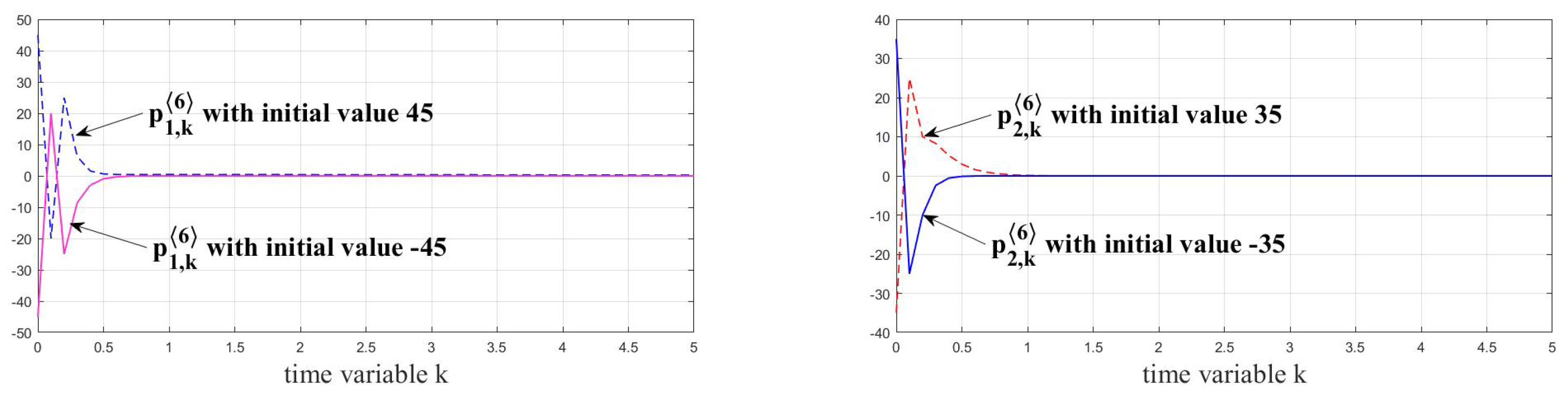
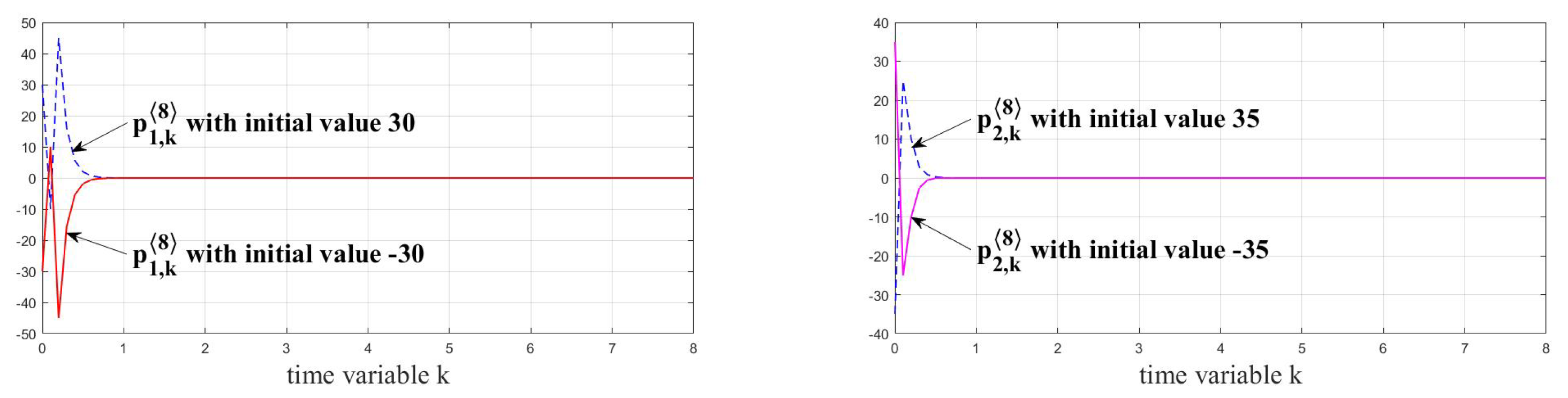
5. Example

This section gives an experimental example to verify the feasibility of the main results for discrete-space and -time stochastic GRNs, which have been addressed in the previous sections of this article.

Considering the following discrete-time stochastic GRNs with discrete spatial diffusions

$$\left\{\begin{array}{cc}\hfill {\displaystyle \left(\begin{array}{c}{\mathbf{m}}_{1,k+1}^{\langle \nu \rangle }\\ {\mathbf{m}}_{2,k+1}^{\langle \nu \rangle }\end{array}\right)=}& \left(\begin{array}{cc}{e}^{-9h}& 0\\ 0& e^{-10h}\end{array}\right)\left(\begin{array}{c}{\mathbf{m}}_{1,k}^{\langle \nu \rangle }\\ {\mathbf{m}}_{2,k}^{\langle \nu \rangle }\end{array}\right)+\left(\begin{array}{cc}\frac{1-e^{-9h}}{9}& 0\\ 0& \frac{1-e^{-10h}}{10}\end{array}\right)[\left(\begin{array}{cc}0.2& 0\\ 0& 0.2\end{array}\right){\tilde{\Delta }}_{\hslash }^2\left(\begin{array}{c}{\mathbf{m}}_{1,k}^{\langle \nu \rangle }\\ {\mathbf{m}}_{2,k}^{\langle \nu \rangle }\end{array}\right)\hfill \\ \hfill & {\displaystyle +\left(\begin{array}{cc}1.2cos(k\pi +\frac{\pi }{4})+e^{-\left|k\right|}& 0.5\\ 0.3& 1.8sin(k\pi +\frac{\pi }{4})+e^{-\left|k\right|}\end{array}\right)\left(\begin{array}{c}{f}_1\left({\mathbf{p}}_{1,k-2}^{\langle \nu \rangle }\right)\\ f_2\left({\mathbf{p}}_{2,k-1}^{\langle \nu \rangle }\right)\end{array}\right)}\hfill \\ \hfill & {\displaystyle +\left(\begin{array}{cc}0.2& 0.1\\ 0& 0.15\end{array}\right)\left(\begin{array}{c}{g}_1\left({\mathbf{p}}_{1,k-1}^{\langle \nu \rangle }\right)w_{11,k}\\ g_2\left({\mathbf{p}}_{2,k-1}^{\langle \nu \rangle }\right)w_{12,k}\end{array}\right)+\left(\begin{array}{c}1+0.2cos(k\pi +\frac{\pi }{4})\\ 0.5+0.5sin(k\pi +\frac{\pi }{4})\end{array}\right)],}\hfill \\ \hfill {\displaystyle \left(\begin{array}{c}{\mathbf{p}}_{1,k+1}^{\langle \nu \rangle }\\ {\mathbf{p}}_{2,k+1}^{\langle \nu \rangle }\end{array}\right)=}& \left(\begin{array}{cc}{e}^{-12h}& 0\\ 0& e^{-15h}\end{array}\right)\left(\begin{array}{c}{\mathbf{p}}_{1,k}^{\langle \nu \rangle }\\ {\mathbf{p}}_{2,k}^{\langle \nu \rangle }\end{array}\right)+\left(\begin{array}{cc}\frac{1-e^{-12h}}{12}& 0\\ 0& \frac{1-e^{-15h}}{15}\end{array}\right)[\left(\begin{array}{cc}0.1& 0\\ 0& 0.1\end{array}\right){\tilde{\Delta }}_{\hslash }^2\left(\begin{array}{c}{\mathbf{p}}_{1,k}^{\langle \nu \rangle }\\ {\mathbf{p}}_{2,k}^{\langle \nu \rangle }\end{array}\right)\hfill \\ \hfill & {\displaystyle +0.1\left(\begin{array}{c}|{\mathbf{m}}_{1,k}^{\langle \nu \rangle }|\\ |{\mathbf{m}}_{2,k}^{\langle \nu \rangle }|\end{array}\right)+\left(\begin{array}{cc}cos(k\pi +\frac{\pi }{3})+e^{-\left|k\right|}& 0.1\\ 0& sin(k\pi +\frac{\pi }{5})+e^{-\left|k\right|}\end{array}\right)\left(\begin{array}{c}{\eta }_1\left({\mathbf{m}}_{1,k-1}^{\langle \nu \rangle }\right)w_{21,k}\\ {\eta }_2\left({\mathbf{m}}_{2,k-2}^{\langle \nu \rangle }\right)w_{22,k}\end{array}\right)],}\hfill \end{array}\right.$$

(22)

where $(\nu ,k)\in (0,10)\times {\mathbb{Z}}_0$,

$${\mathbf{m}}_{i,k}^{\langle \nu \rangle }{|}_{\nu =0}={\mathbf{m}}_{i,k}^{\langle \nu \rangle }{|}_{\nu =10}=0,{\mathbf{p}}_{i,k}^{\langle \nu \rangle }{|}_{\nu =0}={\mathbf{p}}_{i,k}^{\langle \nu \rangle }{|}_{\nu =10}=0,\forall k\in {\mathbb{Z}}_0,i=1,2.$$

Taking $h=0.1$ and $\hslash =0.5$. Corresponding to GRNs Equation (1),

$$a_{1,k}=9,a_{2,k}=10,c_{1,k}=12,c_{2,k}=15,{\mathsf{\Theta }}_{11}={\mathsf{\Theta }}_{22}=0.2,{\Pi }_{11}={\Pi }_{22}=0.1,$$

$${\mathsf{\Theta }}_{12}={\mathsf{\Theta }}_{21}={\Pi }_{12}={\Pi }_{21}=0,b_{11,k}=1.2cos(k\pi +\frac{\pi }{4})+e^{-\left|k\right|},b_{12,k}=0.5,b_{21,k}=0.3,$$

$$b_{22,k}=1.8sin(k\pi +\frac{\pi }{4})+e^{-\left|k\right|},{\sigma }_{1,k}=2,{\sigma }_{2,k}=1,{\gamma }_{11,k}=0.2,{\gamma }_{12,k}=0.1,{\gamma }_{21,k}=0,$$

$${\gamma }_{22,k}=0.15,I_{1,k}=1+0.2cos(k\pi +\frac{\pi }{4}),I_{2,k}=0.5+0.5sin(k\pi +\frac{\pi }{4}),d_{1,k}=d_{2,k}=0.1,$$

$${\varpi }_{11,k}=cos(k\pi +\frac{\pi }{3})+e^{-\left|k\right|},{\varpi }_{12,k}=0.1,{\varpi }_{21,k}=0,{\varpi }_{22,k}=sin(k\pi +\frac{\pi }{5})+e^{-\left|k\right|},$$

$${\displaystyle f_1\left({\mathbf{p}}_{1,k-2}^{\langle \nu \rangle }\right)=\frac{{\left(\frac{{\mathbf{p}}_{1,k-2}^{\langle \nu \rangle }}{15}\right)}^2}{1+{\left(\frac{{\mathbf{p}}_{1,k-2}^{\langle \nu \rangle }}{15}\right)}^2},f_2\left({\mathbf{p}}_{2,k-1}^{\langle \nu \rangle }\right)=\frac{{\left(\frac{{\mathbf{p}}_{2,k-1}^{\langle \nu \rangle }}{15}\right)}^2}{1+{\left(\frac{{\mathbf{p}}_{2,k-1}^{\langle \nu \rangle }}{15}\right)}^2},g_i\left({\mathbf{p}}_{i,k-1}^{\langle \nu \rangle }\right)=\frac{{\left(\frac{{\mathbf{p}}_{i,k-1}^{\langle \nu \rangle }}{20}\right)}^2}{1+{\left(\frac{{\mathbf{p}}_{i,k-1}^{\langle \nu \rangle }}{20}\right)}^2},}$$

$${\eta }_1\left({\mathbf{m}}_{1,k-1}^{\langle \nu \rangle }\right)=\frac{{\left(\frac{{\mathbf{m}}_{1,k-1}^{\langle \nu \rangle }}{10}\right)}^2}{1+{\left(\frac{{\mathbf{m}}_{1,k-1}^{\langle \nu \rangle }}{10}\right)}^2},{\eta }_2\left({\mathbf{m}}_{2,k-2}^{\langle \nu \rangle }\right)=\frac{{\left(\frac{{\mathbf{m}}_{2,k-2}^{\langle \nu \rangle }}{10}\right)}^2}{1+{\left(\frac{{\mathbf{m}}_{2,k-2}^{\langle \nu \rangle }}{10}\right)}^2},i=1,2,\forall (\nu ,k)\in (0,10)\times {\mathbb{Z}}_0.$$

Obviously, $L_1^f=L_2^f=\frac{1}{15}$, $L_1^g=L_2^g=0.05$, $L_1^{\eta }=L_2^{\eta }=0.1$. It follows from the direct calculation that $max\{{\varsigma }_1,{\varsigma }_2\}<1$. Therefore, assumptions $\left({\mathbf{g}}_1\right)$–$\left({\mathbf{g}}_4\right)$ in Theorem 2 are valid, i.e., GRNs Equation (22) possesses a unique weighted pseudo- or $\alpha$-pseudo-almost periodic sequence solution, see Figure 1 and Figure 2. Let ${\widehat{a}}_1=1.25$, ${\widehat{a}}_2=12$, ${\widehat{c}}_1=14$, and ${\widehat{c}}_2=7$. Then, the state feedback controllers corresponding to Equation (14) are listed as follows:

$${\rho }_{1,k}^{\langle ·\rangle }=0.4983{\mathbf{e}}_{1,k}^{\langle ·\rangle },{\rho }_{2,k}^{\langle ·\rangle }=-0.0667{\mathbf{e}}_{2,k}^{\langle ·\rangle },{\varrho }_{1,k}^{\langle ·\rangle }=-0.0546{\mathbf{w}}_{1,k}^{\langle ·\rangle },{\varrho }_{2,k}^{\langle ·\rangle }=0.2735{\mathbf{w}}_{2,k}^{\langle ·\rangle },$$

(23)

where $k\in {\mathbb{Z}}_0.$ Moreover, assumptions $\left({\mathbf{g}}_2\right)$ and $\left({\mathbf{g}}_5\right)$–$\left({\mathbf{g}}_6\right)$ in Theorem 3 hold. Then, the state feedback controller Equation (23) is a finite-time guaranteed cost controller for GRNs Equation (22) with the settling time K satisfying $K<4.0294$, see Figure 3, Figure 4, Figure 5 and Figure 6. Finally, the trajectories of the finite-time exponential stability of GRNs Equation (22) in three-dimensional and two-dimensional spaces are shown in Figure 7, Figure 8, Figure 9 and Figure 10.

In Figure 1 and Figure 2, the pictures show the weighted pseudo-almost periodicity of $\mathbf{m}$ and $\mathbf{p}$ in GRNs Equation (22). From these pictures, we can observe that the solution of GRNs Equation (22) is not weighted pseudo-almost periodic at the beginning of the time, but it becomes almost periodic as the time increases.

In Figure 3 and Figure 4, the pictures show the trajectories of $\mathbf{m}$ and $\mathbf{p}$ in GRNs Equation (22) with feedback controls in the closed loop. By observing these pictures, we can observe that the solutions of GRNs Equation (22) with different initial values realise finite-time exponential stability in three-dimensional space. Figure 5 and Figure 6 give the trajectories of $\mathbf{m}$ and $\mathbf{p}$ of GRNs Equation (22) with feedback controls in the closed loop when $\nu =6$.

Figure 7 and Figure 8 show the solutions of GRNs Equation (22) without feedback control, realising finite-time exponential stability in three-dimensional space. Figure 9 and Figure 10 draw the solutions of GRNs Equation (22) without feedback control, realising finite-time exponential stability when $\nu =8$.

6. Conclusions and Perspectives

Utilizing EED and CFT techniques, discrete stochastic genetic regulatory networks with discrete spatial diffusion are presented, which can be considered as fully discrete configurations of stochastic genetic regulatory networks with reaction diffusion. Based on the constant variable formulation in discrete form, the existence uniqueness, the finite-time guaranteed cost control, and the exponential stability of the weighted pseudo-$\theta$-almost periodic sequence of such discrete stochastic genetic regulatory networks in the mean-square sense are discussed. In addition, Lemmas 2 and 3, among others, have been crucial to the discussion in this paper over the course of the study. Notably, the work in this paper will initiate the development of qualitative problems in discrete-time and discrete-space models, laying the theoretical and practical foundations for future work in this area.

References

- Alon, U. An Introductin to Systems Biology: Design Principles of Biological Circuits; CRC: London, UK, 2006. [Google Scholar]
- Thieffry, D.; Thomas, R. Qualitative analysis of gene networks. Proc. Pac. Symp. Biocomput. 1998, 3, 77–88. [Google Scholar]
- Bao, W.Z.; Yuan, C.A.; Zhang, Y.H. Mutli-features prediction of protein translational modification sites. IEEE/ACM Trans. Comput. Biol. Bioinf. 2018, 15, 1453–1460. [Google Scholar] [CrossRef] [PubMed]
- Somogyi, R.; Sniegoski, C. Modeling the complexity of genetic networks: Understanding multigenic and pleiotropic regulation. Complexity 1996, 1, 45–63. [Google Scholar] [CrossRef]
- de Jong, H. Modeling and simuation of genetic regulatory systems: A literature review. J. Comput. Biol. 2002, 9, 67–103. [Google Scholar] [CrossRef] [PubMed]
- Barabási, A.; Gulbahce, N.; Loscalzo, J. Network medicien: A network-based approach to human disease. Nat. Rev. Genet. 2011, 12, 56–68. [Google Scholar] [CrossRef] [PubMed]
- Song, Q.; Long, L.; Zhao, Z.; Liu, Y.; Alsaadi, F.E. Stability criteria of quatemion-valued neutral-type delayed neural networks. Neurocomputing 2020, 412, 287–294. [Google Scholar] [CrossRef]
- Hood, L.; Health, J.; Phelps, M.; Lin, B. Systems biology and new technologies enable predictive and preventative medicine. Science 2004, 306, 640–643. [Google Scholar] [CrossRef]
- Liu, R.J.; Lu, J.Q.; Lou, J.G.; Alsaedi, A.; Alsaedi, F.E. Set stabiliation of Boolean networks under pinning contril strategy. Neurocomputing 2017, 260, 142–148. [Google Scholar] [CrossRef]
- Possieri, C.; Teel, A.R. Asymptotic stability in probability for stochastic Boolean Networks. Automatica 2017, 83, 1–9. [Google Scholar] [CrossRef]
- Zhang, X.Y.; Wang, Y.T.; Zhang, X. Improved stochastic integral inequalities to stability analysis of stochastic genetic regulatory networks with mixed time-varying delays. IET Control Theory Appl. 2020, 14, 2439–2448. [Google Scholar] [CrossRef]
- Ayachi, M. Existence and exponential stability of weighted pseudo-almost periodic solutions for genetic regulatory networks with time-varying delays. Int. J. Biomath. 2021, 14, 2150006. [Google Scholar] [CrossRef]
- Chen, T.; He, H.Y.; Church, G.M. Modeling gene expression with differential equations. Pac. Symp. Biocomput. 1999, 4, 29–40. [Google Scholar]
- Han, Y.Y.; Zhang, X.; Wang, Y.T. Asymptotic Stability Criteria for genetic regulatory networks with time-varying delays and reaction-diffusion terms. Circ. Syst. Signal Process 2015, 34, 3161–3190. [Google Scholar] [CrossRef]
- Zou, C.Y.; Zhou, C.J.; Zhang, Q.; He, V.Y.; Huang, C. State emstimation for delayed genetic regulatory networks with reaction diffusion terms and Markovian jump. Complex Intell. Syst. 2023, 1–15. [Google Scholar] [CrossRef]
- Xie, Y.P.; Xiao, L.; Wang, L.M.; Wang, G.H. Algebriaic Stability Criteria of Reaction Diffusion Genetic Regulatory Neteorks With Discrete and Distrubted Delays. IEEE Access 2021, 9, 16410–16418. [Google Scholar] [CrossRef]
- Xue, Y.; Liu, C.Y.; Zhang, X. State bounding description and reachable set estimation for discrete-time genetic regulatory networks with time-varying delays and bounded disturbances. IEEE Trans. Syst. Man Cybern. Syst. 2022, 52, 6652–6661. [Google Scholar] [CrossRef]
- Liu, C.Y.; Wang, X.; Xue, Y. Global exponential stability analysis of discrete-time genetic regulatory networks with time-varying discrete delays and unbounded distributed delays. Neurocomputing 2020, 372, 100–108. [Google Scholar] [CrossRef]
- Yue, D.D.; Guan, Z.H.; Chen, J.; Ling, G.; Wu, Y. Bifurcations and chaos of a discrete-time model in genetic regulatory networks. Nonlinear Dyn. 2017, 87, 567–586. [Google Scholar] [CrossRef]
- Zhang, T.W.; Li, Y.K. Global exponential stability of discrete-time almost automorphic Caputo—Fabrizio BAM fuzzy neural networks via exponential Euler technique. Knowl.-Based Syst. 2022, 246, 108675. [Google Scholar] [CrossRef]
- Huang, Z.K.; Mohamad, S.; Gao, F. Multi-almost periodicity in semi-discretizations of a general class of neural networks. Math. Comput. Simul. 2014, 101, 43–60. [Google Scholar] [CrossRef]
- Zhang, T.W.; Han, S.F.; Zhou, J.W. Dynamic behaviours for semi-discrete stochastic Cohen-Grossberg neural networks with time delays. J. Frankl. Inst. 2020, 357, 13006–13040. [Google Scholar] [CrossRef]
- Zhang, T.W.; Qu, H.Z.; Liu, Y.T.; Zhou, J.W. Weighted pseudo θ-almost periodic sequence solution and guaranteed cost control for discrete-time and discrete-space stochastic inertial neural networks. Chaos Solitons Fractals 2023, 173, 113658. [Google Scholar] [CrossRef]
- Zhang, T.W.; Li, Z.H. Switching clusters’ synchronization for discrete space-time complex dynamical networks via boundary feedback controls. Pattern Recognit. 2023, 143, 109763. [Google Scholar] [CrossRef]
- Zhang, T.W.; Liu, Y.T.; Qu, H.Z. Global mean-square exponential stability and random periodicity of discrete-time stochastic inertial neural networks with discrete spatial diffusions and Dirichlet boundary condition. Comput. Math. Appl. 2023, 141, 116–128. [Google Scholar] [CrossRef]
- Xu, G.X.; Bao, H.B.; Cao, J.D. Mean-square exponential input-to-state stability of stochastic gene regulatory networks with maltiple time delays. Neural Process. Lett. 2020, 51, 271–286. [Google Scholar] [CrossRef]
- Zhou, J.; Xu, S.; Shen, H. Finite-time robust stochastic stability of uncertain stochastic delayed reaction-diffusion genetic regulatory networks. Neurocomputing 2011, 74, 2790–2796. [Google Scholar] [CrossRef]
- Wang, W.Q.; Zhong, S.M.; Liu, F. Robust filtering of uncertain stochastic genetic regulatory networks with time-varying delays. Chaos Solitons Fract. 2012, 45, 915–929. [Google Scholar] [CrossRef]
- Wang, B. Random periodic sequence of globally mean-square exponentially stable discrete-time stochastic genetic regulatory networks with discrete spatial diffusions. Electron. Res. Arch. 2023, 31, 3097–3122. [Google Scholar] [CrossRef]
- Zhang, G.P.; Zhu, Q.X. Finite-time guaranteed cost control for uncertain delayed switched nonlinear stochastic systems. J. Frankl. Institeu 2022, 359, 8802–8818. [Google Scholar] [CrossRef]
- Gao, H.; Zhang, H.B.; Shi, K.B.; Zhou, K. Event-triggered finite-time guaranteed cost control for networked Takagi-Sugeno (T-S) fuzzy switched systems under denial of service attacks. Int. J. Robust Nolinear Control 2022, 32, 5764–5775. [Google Scholar] [CrossRef]
- Liu, L.P.; Di, Y.F.; Shang, Y.L.; Fu, Z.M.; Fan, B. Guaranteed Cost and Finite-Time Non-fragile Control of Fractional-Order Positive Switched Systems with Asynchronous Switching and Impulsive Moments. Circuits Syst. Signal Process. 2021, 40, 3143–3160. [Google Scholar] [CrossRef]
- Liu, M.X.; Wu, B.W.; Wang, Y.E.; Liu, L.L. Dynamic Output Feedback Control and Guaranteed Cost Finite-time Boundedness for Uncertain Switched Linear Systems. Int. J. Control Autom. Syst. 2023, 21, 400–409. [Google Scholar] [CrossRef]
- Liu, M.X.; Wu, B.W.; Wang, Y.E.; Liu, L.L. Dynamic Output Feedback control and Guaranteed Cost Finite-Time Boundedness for Switched Linear Systems. Circuits Syst. Signal Process. 2022, 41, 2653–2668. [Google Scholar] [CrossRef]
- Liu, X.K.; Li, W.C.; Yao, C.X.; Li, Y. Finite-Time Guaranteed Cost Control for Markovian Jump Systems with Time-Varying Delays. Mathematics 2022, 10, 2028. [Google Scholar] [CrossRef]
- Zhang, X.; Yin, Y.Y.; Wang, H.; He, S.P. Finite-time dissipative control for time-delay Markov jump systems with conic-type non-linearities under guaranteed cost controller and quantiser. IET Control Theory Appl. 2021, 15, 489–498. [Google Scholar] [CrossRef]
- Luo, Y.P.; Wang, X.E.; Cao, J.D. Guaranteed-cost finite-time consensus of multi-agent systems via intermittent control. Math. Methods Appl. Sci. 2022, 45, 697–717. [Google Scholar] [CrossRef]
- Duan, L.; Di, F.J.; Wang, Z.Y. Existence and global exponential stability of almost periodic solutions of genetic regulatory networks with time-varying delays. J. Exp. Theor. Artif. Intell. 2020, 32, 453–463. [Google Scholar] [CrossRef]
- Luo, Q.; Zhang, R.B.; Liao, X.X. Unconditional global exponential stability in Lagrange sense of genetic regulatory networks with SUM regulatory logic. Cogn. Neurodyn. 2010, 4, 251–261. [Google Scholar] [CrossRef]
- Li, Y.J.; Zhang, X.; Tan, C. Global exponential stability analysis of discrete-time genetic regulatory networks with time delays. Asian J. Control 2013, 15, 1448–1475. [Google Scholar] [CrossRef]
- Xie, Y.P.; Xiao, L.; Ge, M.F.; Wang, L.M.; Wang, G.H. New results on global exponential stability of genetic regulatory networks with diffusion effect and time-varying hybird delays. Neural Process. Lett. 2021, 53, 3947–3963. [Google Scholar] [CrossRef]
- Liu, Z.X.; Yang, X.; Yu, T.T.; Zhang, X.; Wang, X. Global Exponential Satbility Analysis of Coupled Cyclic Genentic Regulatory Networks With Constant Delays. IEEE Trans. Control Netw. Syst. 2021, 8, 1811–1821. [Google Scholar] [CrossRef]
- Zhang, W.L.; Zheng, Z.H. Random almost periodic solutions of random dynamical systems. arXiv 2019, arXiv:1909.01586. [Google Scholar]
- de Fitte, P.R. Almost periodicity and periodicity for nonautonomous random dynamical systems. Stochastics Dyn. 2020, 21, 2150034. [Google Scholar] [CrossRef]
- Marie, N.; Fitte, P.R.D. Almost periodic and periodic solutions of differential equations driven by the fractional Brownian motion with statistical application. Stochastics 2020, 93, 886–906. [Google Scholar] [CrossRef]
- Zhang, C. Pseudo almost periodic solutions of some differential equations. J. Math. Anal. Appl. 1994, 181, 62–76. [Google Scholar] [CrossRef]
- Diagana, T. Weighted pseudo-almost periodic functions and applications. Comptes Rendus Math. 2006, 343, 643–646. [Google Scholar] [CrossRef]
- Es-saiydy, M.; Zitane, M. New composition theorem for weighted stepanov-like pseudo almost periodic functions on time scales and applications. Bol. Soc. Parana. Mat. 2023, in press. [CrossRef]
- Yan, Z. Sensitivity analysis for a fractional stochastic differential equation with S-p-weighted pseudo almost periodic coefficients and infinite delay. Fract. Calc. Appl. Anal. 2022, 25, 2356–2399. [Google Scholar] [CrossRef]
- M’Hamdi, M.S. On the weighted pseudo almost-periodic solutions of static DMAM neural network. Neural Process. Lett. 2022, 54, 4443–4464. [Google Scholar] [CrossRef]
- Hu, P.; Huang, C.M. Delay dependent asymptotic mean square stability analysis of the stochastic exponential Euler method. J. Comput. Appl. Math. 2021, 382, 113068. [Google Scholar] [CrossRef]
- Zhang, T.W.; Li, Y.K. Exponential Euler scheme of multi-delay Caputo-Fabrizio fractional-order differential equations. Appl. Math. Lett. 2022, 124, 107709. [Google Scholar] [CrossRef]
- Bessaih, H.; Garrido-Atienza, M.J.; Köpp, V.; Schmalfuß, B.; Yang, M. Synchronization of stochastic lattice equations. Nonlinear Differ. Equ. Appl. Nodea 2020, 27, 36. [Google Scholar] [CrossRef]
- Han, X.Y.; Kloeden, P.E. Sigmoidal approximations of Heaviside functions in neural lattice models. J. Differ. Equ. 2020, 268, 5283–5300. [Google Scholar] [CrossRef]
- Han, X.Y.; Kloden, P.E.; Usman, B. Upper semi-continuous convergence of attractors for a Hopfield-type lattice model. Nonlinearity 2020, 33, 1881–1906. [Google Scholar] [CrossRef]
- Kuang, J.C. Applied Inequalities; Shandong Science and Technology Press: Shandong, China, 2012. [Google Scholar]
- Arnold, L. Random Dynamical Systems; Springer: Berlin, Germany, 1998. [Google Scholar]
Disclaimer/Publisher’s Note: The statements, opinions and data contained in all publications are solely those of the individual author(s) and contributor(s) and not of MDPI and/or the editor(s). MDPI and/or the editor(s) disclaim responsibility for any injury to people or property resulting from any ideas, methods, instructions or products referred to in the content. |
© 2023 by the authors. Licensee MDPI, Basel, Switzerland. This article is an open access article distributed under the terms and conditions of the Creative Commons Attribution (CC BY) license (https://creativecommons.org/licenses/by/4.0/).
Share and Cite
Sun, S.; Zhang, T.; Li, Z. Weighted Pseudo-θ-Almost Periodic Sequence and Finite-Time Guaranteed Cost Control for Discrete-Space and Discrete-Time Stochastic Genetic Regulatory Networks with Time Delays. Axioms 2023, 12, 682. https://doi.org/10.3390/axioms12070682
Sun S, Zhang T, Li Z. Weighted Pseudo-θ-Almost Periodic Sequence and Finite-Time Guaranteed Cost Control for Discrete-Space and Discrete-Time Stochastic Genetic Regulatory Networks with Time Delays. Axioms. 2023; 12(7):682. https://doi.org/10.3390/axioms12070682
Chicago/Turabian StyleSun, Shumin, Tianwei Zhang, and Zhouhong Li. 2023. "Weighted Pseudo-θ-Almost Periodic Sequence and Finite-Time Guaranteed Cost Control for Discrete-Space and Discrete-Time Stochastic Genetic Regulatory Networks with Time Delays" Axioms 12, no. 7: 682. https://doi.org/10.3390/axioms12070682