Article

A Time-Varying Coefficient Double Threshold GARCH Model with Explanatory Variables

1
School of Economics, Liaoning University, Shenyang 110036, China
2
School of Mathematics and Statistics, Liaoning University, Shenyang 110036, China
*
Authors to whom correspondence should be addressed.
Axioms 2023, 12(5), 476; https://doi.org/10.3390/axioms12050476
Submission received: 25 March 2023 / Revised: 5 May 2023 / Accepted: 11 May 2023 / Published: 15 May 2023
(This article belongs to the Special Issue Mathematical and Statistical Methods and Their Applications)

Abstract

:
In this article, we consider the nonparametric inference for the time-varying coefficient double-threshold generalized autoregressive conditional heteroscedastic models. The quasi-maximum exponential likelihood estimators (QMELEs) of the model’s parameters and the asymptotic properties of the estimators are obtained. The simulation study implies that the distribution of the estimators is asymptotically normal. A real data application to stock returns is given. Both the simulations and real data example imply that the model and the QMELE are proper, compatible and accurately fit the financial time series data of the Nikkei 225.

1. Introduction

The random coefficient autoregressive (RCA) model proposed by [1] is a nonlinear time series models that is widely used when analyzing data generated on economics and finance. The RCA model incorporates a random variable in its autoregressive coefficient part, and thus makes the model able to capture the random influential factors. Refs. [2,3,4,5] studied various problems of inference for non-linear time-series models, including random coefficient models. Subsequently, ref. [6] proposed the generalized random coefficient autoregressive (GRCA) model. Refs. [7,8] studied properties of the RCA model with order 1 (the RCA(1) model). Ref. [9] studied the RCA model with GARCH innovations and its properties.
When analyzing the economic and financial time series, researchers found that the data frequently exhibit apparent evidence of asymmetry. For example, when the stock price is rising (in a bull market), the return yield (volatility) is different from the relevant yield when the price is falling (in a bear market). Refs. [10,11] proposed the threshold autoregressive model (TAR) to capture the asymmetric features shown in the financial time series. By using the threshold variable, the TAR model set up several different regimes with different parameters to describe asymmetric phenomena. Since [12] proposed the autoregressive conditional heteroscedastic (ARCH) model and [13] extended the ARCH models to the generalized autoregressive conditional heteroscedastic (GARCH) models, ref. [14] implied that the asymmetric volatility is exhibited in financial series data obtained from the stock market. Ref. [15] extended the TAR model to the model with conditional heteroscedasticity, which is the self-exciting threshold autoregressive ARCH (SETAR-ARCH) model. Then, ref. [16] proposed the double-threshold autoregressive conditional heteroscedastic (DTARCH) model, which captures asymmetry in the conditional mean and conditional variance at the same time, and used their model to analyze the Hang Seng Index return series in Hong Kong. Ref. [17] extended the DTARCH model to the DTGARCH model and used it to investigate the French Franc/Deutschmark exchange rates. Based on these achievements, several researchers conducted further studies of applications of this model in finance and economics, e.g., [18,19,20,21,22].
In the literature related to the RCA model, the random coefficient is usually affected by an independent and identically distributed random variable. In [1], the random coefficient part is influenced by a white noise sequence. However, in practical application, the random coefficients may depend on some observed data and external factors. For instance, when analyzing the stock data, the return of yield at time t should be influenced by the one at time t 1 and some factors external to the stock market. Ref. [23] proposed the smooth transition autoregressive (STAR) model, and the autoregressive parameters of STAR model incorporated the influence of the observations. Then, ref. [24] used the smooth transition autoregressive (STAR) model to analyze the data of industrial production in West Germany. Since then, STAR models have widely been used in economics and finance. When analyzing the economic and financial data, the models are not only affected by observations but also some external factors. Therefore, incorporating the observations and explanatory variables in the model and influencing the model through the random coefficient part are considered. Refs. [25,26,27] proposed several integer-valued autoregressive models, in which the random coefficients were influenced by observations or explanatory variables. Motivated by the above literature, which shows different approaches of constructing time series models, we incorporate observations and explanatory variables into the autoregressive coefficient part, and investigate a time-varying coefficient double-threshold generalized autoregressive conditional heteroscedastic (TVCDT-GARCH) model.
Ref. [28] studied the estimation of the random coefficient AR(1) processes based on the least squares estimator. Ref. [8] studied the model parameter estimation of the RCA(1) model, and [9] discussed the RCA models with GARCH innovations and its parameter-estimation problem. Ref. [29] found that some parameters of the nonstationary RCA model cannot be estimated using quasi-maximum likelihood estimation (QMLE); then, ref. [30] presented the quasi-likelihood estimation for the stationary and nonstationary process of RCA(1) model. In general, when solving the problem related to the model parameter estimation of the G/ARCH type model, the QMLE is an approach that is frequently used and is discussed by several researchers, such as [31,32,33,34]. However, QMLE requires a finite fourth moment for the error term. Due to the heavy-tailed features of financial time series, this requirement is not easily satisfied in many practical applications, especially in economics and finance. Ref. [35] studied the models with heavy-tailed errors and showed that QMLE is not asymptotically normal. Then, ref. [36] proposed the quasi-maximum exponential likelihood estimators (QMELE) for the ARMA-GARCH model under a fractional moment condition of the error term without specification of the distribution of the error term. Consequently, QMELE exhibits superior performance when dealing with heavy-tailed data in practical applications. These considerations motivate us to study the QMELE of the TVCDT-GARCH model.
As financial data usually involve non-normality and fat tails, the double exponential distribution is better than the normal distribution for characterizing heavy-tailed data. Compared with traditional QMLE, the QMELE is a better approach to esimate model parameters. The time-varying coefficients of our model incorporate not only the information of observations but also the information of external factors. Hence, by using QMELE, we investigate inference for TVCDT-GARCH models, which provides practitioners with an attractive modeling alternative for fitting financial data.
The rest of this paper is organized as follows. In Section 2, we discuss the model, parameter estimation and the asymptotic results. Section 3 shows the results from some simulation studies. In Section 4, we use our results to analyze the real data of the Nikkei 225. Section 5 provides our conclusions and some extensions for further research. We put the proofs in Appendix A.

2. Model and Estimation

Ref. [1] proposed the classic random coefficient autoregressive (RCA) model as the following:
y t = ( φ + b t ) y t 1 + ϵ t , t N .
where ( b t , ϵ t ) are independent and identically distributed pairs of random variables and satisfy
E ( b t , ϵ t ) = ( 0 , 0 ) , c o v ( b t , ϵ t ) = σ b 2 0 0 σ ϵ 2 .
Although the RCA models are widely used in biology, economics and finance, and studied in the literature, there are some drawbacks that can be improved. For instance, when analyzing stock data, the return of yield at time t should be influenced by the one at time t 1 and some external factors; however, in the RCA model, the random coefficient is only affected by the random variable b t . Based on the discussion above, we consider the following time-varying coefficient double threshold GARCH (TVCDT-GARCH) model:
y t = i = 1 p ϕ i , t ( 1 ) y t i + ϵ t , y t d r , i = 1 p ϕ i , t ( 2 ) y t i + ϵ t , y t d > r , ϵ t = η t h t ,
h t = ω 1 + i = 1 q α 1 i ϵ 1 t i 2 + i = 1 s β 1 i h 1 t i , y t d r , ω 2 + i = 1 q α 2 i ϵ 2 t i 2 + i = 1 s β 2 i h 2 t i , y t d > r ,
where
ln ϕ i , t ( j ) 1 ϕ i , t ( j ) = c j , i y t 1 + d j z t ,
where z t represents observations of explanatory variables, { z t } is a stationary sequence, j = { 1 , 2 } , i = { 1 , 2 , , n } , d p , p , q , s and d are positive integers, { η t } are independent and identically distributed noise with E | η t | = 1 , and r is a threshold parameter. Let θ = ( c , δ , r ) be the model parameters with true value θ 0 = ( c 0 , δ 0 , r 0 ) , where δ = ( ω 1 , α 11 , , α 1 q , β 11 , , β 1 s , ω 2 , α 21 , , α 2 q , β 21 , , β 2 s ) and c = ( c 11 , , c 1 p , d 1 , c 21 , , c 2 p , d 2 ) . The parameter space is Θ = Θ c × Θ δ × Θ r , where Θ c R 2 ( p + 1 ) , Θ δ R 0 2 ( q + s + 1 ) , Θ r R , R = ( , ) , R 0 = [ 0 , ) . For the sake of representation, let λ = ( c , δ ) denote the parameters in our model, except the threshold parameter r; then, Θ λ = Θ c × Θ δ . Assume that Θ c and Θ δ are compact, and θ 0 is an interior point of Θ . We consider the following function:
L n ( θ ) = t = 1 n l t ( θ ) , w i t h l t ( θ ) = { l o g h 1 t ( θ ) + | ϵ 1 t | h 1 t ( θ ) } I 1 t + { l o g h 2 t ( θ ) + | ϵ 2 t | h 2 t ( θ ) } I 2 t ,
where I 1 t = I ( y t d r ) and I 2 t = I ( y t d > r ) . We look for θ ^ n , the minimizer of L n ( θ ) on Θ , where
θ ^ n = arg min Θ L n ( θ ) .
θ ^ n is called the QMELE of θ 0 . To estimate θ ^ n , we have to fix the threshold parameter r, then minimize L n ( θ ) on Θ λ and finally derive its minimizer λ ^ n ( r ) . In what follows, we assume that r is already known.
In the circumstances that r is unknown, we can use several methods to estimate the threshold parameter, such as the single grid search (SGS) algorithm (e.g., [37,38,39]) and the nested sub-sample search (NeSS) algorithm ([40]), etc. Researchers then can choose a proper method to locate the threshold parameter. Using the optimization algorithms to optimize the log-likelihood function is an alternative procedure to obtain the threshold parameter. Whether this estimator is proper or not requires judgement. We use the SGS method to estimate the threshold parameter r in our estimation process. When r is fixed, we can calculate the AIC of the model, and the optimal r is the one with the minimum model AIC. Using the SGS method, we search for r over the range of the 20th to the 80th percentile of the sample data with a search step size of 0.01 (1%), and then we obtain the estimated threshold r ^ that corresponds to the minimum model AIC.
Remark 1.
The least absolute deviation (LAD) estimation can also relax the requirement of the moment condition. However, we do not use the LAD method to estimate the parameters of our model. Remark 2.2 in [41] gives a detailed description, and thus we will not consider the LAD method henceforward.
Next, we discuss the asymptotic properties of our estimators. Let A j ( z ) = i = 1 q α j i z i , and B j ( z ) = 1 i = 1 s β j i z i . We need the following assumptions.
Assumption 1.
{ y t } satisfying Equation (1) is strictly stationary and ergodic. The parameter space Θ is compact. ω j > 0 , α j i > 0 , β j i > 0 , i = 1 q α j i + i = 1 s β j i < 1 for i = 1 , 2 , , and j = 1 , 2 .
Assumption 2.
For each θ Θ , A j ( z ) and B j ( z ) have no common root, A j ( 1 ) 0 , α q + β s 0 , and we let A j = ( α j 1 , , α j q ) , A j A j if j j . A similar condition holds for B j = ( β j 1 , , β j s ) , Φ j = ( ϕ j 1 , , ϕ j p ) and ω j .
Assumption 3.
η t 2 has a nondegenerate distribution with E η t 2 < . { η t } is independent and identically distributed with median 0, E | η t | = 1 ; its density function f ( x ) is continuous and satisfies f ( 0 ) > 0 , sup x R f ( x ) < , and sup x R | f ( x ) | < .
Assumption 4.
E [ ξ ρ t 1 3 ] < for any ρ ( 0 , 1 ) , where ξ ρ t = 1 + i = 1 ρ i | y t i | .
Assumption 5.
sup ( y , z ) R 2 | c j , i y + d j z | < , j = { 1 , 2 } , i = { 1 , 2 , . . . . . , p } , and { z t } is a stationary sequence and independent of { ϵ t } .
Remark 2.
For the time-varying coefficients part, we notice that 0 < ϕ i , t ( j ) = e x p ( c j , i y t 1 + d j z t ) e x p ( c j , i y t 1 + d j z t ) + 1 < 1 , j = { 1 , 2 } , i = { 1 , 2 , , p } . With Assumptions 1–5 and similarly to Proposition 1.1 in [42], the parameters of the autoregressive part fit the strictly stationary and ergodic solution condition. Our model is a two-regime threshold model that can be seen as a special case of [43] that then combines the corresponding results of Theorem 1 in [43] with the restrictions on the parameters of the variance part: ω j > 0 , α j i > 0 , β j i > 0 , i = 1 q α j i + i = 1 s β j i < 1 . We can guarantee the stationarity of our model.
For the sake of clarity, let θ ^ s n denote the minimizer of L n ( θ ) on Θ λ for fixed r. The following theorem gives the strong consistency of θ ^ s n .
Theorem 1.
Suppose η t has a zero median with E | η t | = 1 . If Assumptions 1–5 hold, then θ ^ s n θ 0 a.s., as n .
To investigate the rate of convergence of θ ^ s n , we rewrite the log-likelihood function as follows: H n ( u , r ) L n ( λ 0 + u , r ) L n ( λ 0 , r ) , where u { u = ( u 1 , u 2 ) : u + λ 0 Θ λ } ( u i = ( u i 1 , u i 2 , , u i ( p + q + s + 2 ) ) , i = 1 , 2 . ) . Let u ^ n ( r ) = λ ^ ( r ) λ 0 ; then, u ^ n ( r ) is the minimizer of H n ( u , r ) for fixed r. Note that
H n ( u , r ) = H n ( u , r 0 ) + H n ( u , r ) H n ( u , r 0 ) ,
and
H n ( u , r 0 ) = L n ( λ 0 + u , r 0 ) L n ( λ 0 , r 0 ) = i = 1 2 L ˜ i n ( u i , r 0 ) ,
where
L ˜ i n ( u i , r 0 ) = t = 1 n { l o g h i t ( θ 0 + u ) + | ϵ i t ( γ 0 + u i ) | h i t ( θ 0 + u ) l o g h i t ( θ 0 ) | ϵ i t ( γ 0 ) | h i t ( θ 0 ) } I i t .
Now we divide L ˜ i n ( u i , r 0 ) into three parts:
L ˜ i n ( u i , r 0 ) = t = 1 n A i t ( u i , r 0 ) + t = 1 n B i t ( u i , r 0 ) + t = 1 n C i t ( u i , r 0 ) ,
where
A i t ( u i , r 0 ) = 1 h i t ( θ 0 ) [ | ϵ i t ( γ 0 + u 1 ) | | ϵ i t ( γ 0 ) | ] I i t , B i t ( u i , r 0 ) = { l o g h i t ( θ 0 + u ) l o g h i t ( θ 0 ) + | ϵ i t ( γ 0 ) | h i t ( θ 0 + u ) | ϵ i t ( γ 0 ) | h i t ( θ 0 ) } I i t , C i t ( u i , r 0 ) = [ 1 h i t ( θ 0 + u ) 1 h i t ( θ 0 ) ] [ | ϵ i t ( γ 0 + u 1 ) | | ϵ i t ( γ 0 ) | ] I i t .
Let F t 1 = σ { η t 1 , η t 2 , } ; using the equality
| x y | | x | = y [ I ( x > 0 ) I ( x < 0 ) ] + 2 0 y [ I ( x s ) I ( x 0 ) ] d s ,
we have
A i t ( u i , d 0 ) = s i t ( u i ) [ I ( η t > 0 ) I ( η t < 0 ) ] + 2 0 s i t ( u i ) [ I ( η t s ) I ( η t 0 ) ] d s , where s i t ( u i ) = s i t ( 1 ) ( u i ) + s i t ( 2 ) ( u i ) ,
s i t ( 1 ) ( u i ) = u i I i t h i t ( θ 0 ) ϵ i t ( γ 0 ) θ , s i t ( 2 ) ( u i ) = u i I i t 2 h i t ( θ 0 ) 2 ϵ i t ( γ * ) θ θ u i ,
and γ * lies between γ 0 and γ 0 + u i . Let ξ i t ( u i ) = 0 s i t ( u i ) [ I ( η t s ) I ( η t 0 ) ] d s , and note that I ( η t > 0 ) I ( η t < 0 ) = s g n ( η t ) ; then, we have
t = 1 n A i t ( u i , r 0 ) = u i T i n ( 1 ) + Π i n ( 1 ) ( u i ) + Π i n ( 2 ) ( u i ) + Π i n ( 3 ) ( u i ) ,
where
T i n ( 1 ) = t = 1 n I i t h i t ( θ 0 ) ϵ i t ( γ 0 ) θ s g n ( η t ) , Π i n ( 1 ) ( u ) = 2 t = 1 n { ξ i t ( u i ) E [ ξ i t ( u i ) | F t 1 ] } , Π i n ( 2 ) ( u ) = 2 t = 1 n E [ ξ i t ( u i ) | F t 1 ] , a n d Π i n ( 3 ) ( u ) = t = 1 n s i t ( 2 ) ( u i ) s g n ( η t ) .
By Taylor’s expansion, we have
t = 1 n B i t ( u i , r 0 ) = u T i n ( 2 ) + Π i n ( 4 ) ( u i ) + Π i n ( 5 ) ( u i ) ,
where
T i n ( 2 ) = t = 1 n I i t 2 h i t ( θ 0 ) h i t ( θ 0 ) θ ( 1 | η t | ) , Π i n ( 4 ) ( u i ) = u i t = 1 n ( 3 8 | ϵ i t ( γ 0 ) h i t ( θ * ) | 1 4 ) I i t h i t 2 ( θ * ) h i t ( θ * ) θ h i t ( θ * ) θ u i , Π i n ( 5 ) ( u i ) = u i t = 1 n ( 1 4 1 4 | ϵ i t ( γ 0 ) h i t ( θ * ) | ) I i t h i t ( θ * ) 2 h i t ( θ * ) θ θ u i ,
and θ * lies between θ 0 and θ 0 + u . We need three lemmas.
Lemma 1.
Let T i n = T i n ( 1 ) + T i n ( 2 ) for i = 1, 2. If Assumptions 1–5 hold, then
1 n T i n d N ( 0 , Ω i ) a s n ,
where
Ω i = E ( I i t h i t ( θ 0 ) ϵ i t ( γ 0 ) θ ϵ i t ( γ 0 ) θ ) E η t 2 E ( I i t [ h i t ( θ 0 ) ] 3 2 ϵ i t ( γ 0 ) θ h i t ( θ 0 ) θ ) E η t 2 E ( I i t [ h i t ( θ 0 ) ] 3 2 ϵ i t ( γ 0 ) θ h i t ( θ 0 ) θ ) E η t 2 1 4 E ( I i t h i t 2 ( θ 0 ) h i t ( θ 0 ) θ h i t ( θ 0 ) θ ) .
Lemma 2.
If Assumptions 1–5 hold, then for any sequence of random variables a n such that a n = o p ( 1 ) , it follows that, for i = 1, 2,
( a ) Π i n ( 1 ) ( a n ) = o p ( n a n + n a n 2 ) , ( b ) Π i n ( 2 ) ( a n ) = ( n a n ) Σ i ( 1 ) ( n a n ) + o p ( n a n 2 ) , ( c ) Π i n ( 3 ) ( a n ) = o p ( n a n 2 ) , ( d ) Π i n ( 4 ) ( a n ) = ( n a n ) Σ i ( 2 ) ( n a n ) + o p ( n a n 2 ) , ( e ) Π i n ( 5 ) ( a n ) = o p ( n a n 2 ) , ( f ) t = 1 n C i t ( a i , d 0 ) = o p ( n a n 2 ) ,
where
Σ i ( 1 ) = f ( 0 ) E ( I i t h i t ( θ 0 ) ϵ i t ( γ 0 ) θ ϵ i t ( γ 0 ) θ ) , Σ i ( 2 ) = 1 8 E ( I i t h i t 2 ( θ 0 ) h i t ( θ 0 ) θ h i t ( θ 0 ) θ ) .
Lemma 3.
If Assumptions 1–5 hold, then
sup r r 0 B / n | H n ( u ^ n ( r ) , r ) H n ( u ^ n ( r ) , r 0 ) | = o p ( sup r r 0 B / n n u ^ n ( r ) ) .
Then, we can establish the asymptotic normality of θ ^ s n .
Theorem 2.
If Assumptions 1–5 hold, then
(1) n ( θ ^ s n θ 0 ) = O p ( 1 ) as n ,
(2) n ( θ ^ s n θ 0 ) d N ( 0 , 1 4 Σ 0 1 Ω 0 Σ 0 1 ) as n ,
where Σ 0 = d i a g ( Σ 1 , Σ 2 ) and Ω 0 = d i a g ( Ω 1 , Ω 2 ) with Σ i = d i a g { Σ i ( 1 ) , Σ i ( 2 ) } ,
for i = 1 , 2 .
The proofs of Lemmas and Theorems are given in Appendix A.
When we analyze the real data of the Nikkei 225, we calculate the asymptotic standard deviation using χ ^ n = 1 4 Σ ^ n 1 Ω ^ n Σ ^ n 1 , where Σ ^ n = d i a g ( Σ ^ 1 , Σ ^ 2 ) and Ω ^ n = d i a g ( Ω ^ 1 , Ω ^ 2 ) . For i = 1 , 2 , Σ ^ i and Ω ^ i are estimated by
Σ ^ i n = d i a g { f ^ ( 0 ) κ ^ i n ( 1 ) , 1 8 κ ^ i n ( 2 ) } , Ω ^ i n = κ ^ i n ( 1 ) 1 2 μ ^ κ ^ i n ( 3 ) 1 2 μ ^ κ ^ i n ( 3 ) 1 4 ( ν ^ 1 ) κ ^ i n ( 2 ) ,
where
κ ^ i n ( 1 ) = 1 n t = 1 n I i t h i t ( θ ^ n ) ϵ i t ( γ ^ n ) θ ϵ i t ( γ ^ n ) θ , κ ^ i n ( 2 ) = 1 n t = 1 n I i t h i t 2 ( θ ^ n ) h i t ( θ ^ n ) θ h i t ( θ ^ n ) θ , κ ^ i n ( 3 ) = 1 n t = 1 n I i t [ h i t ( θ ^ n ) ] 3 2 ϵ i t ( γ ^ n ) θ h i t ( θ ^ n ) θ , μ ^ = 1 n t = 1 n η ^ t , ν ^ = 1 n t = 1 n η ^ t 2 .
We can obtain f ^ ( 0 ) from the following function:
f ^ ( 0 ) = 1 n b n t = 1 n K ( η ^ t b n ) ,
where K ( x ) is the kernel function and b n is the bandwidth. In the simulation study, we choose the normal kernel function and a same bandwidth with [44], b = 1.06 · s n 0.2 , where s is the sample standard deviation. By replacing the true value θ 0 with our estimator θ ^ s n in theoretical asymptotic variance, we obtain the consistent asymptotic variance estimation. Researchers can flexibly use the results above to work on the studies they are interested in, such as constructing confidence intervals or test procedure to study some statistical test problems, based on their own requirements.

3. Simulation Studies

In this section, we compare the estimation performance results of QMELE and QMLE under the circumstances that the error terms follow different distributions. The data-generating processes (DGPs) are as follows.
D G P 1 :
y t = ϕ 1 t · y t 1 + η t 0.3 + 0.2 · ϵ 1 t 1 2 + 0.4 · h 1 t 1 , y t 1 1 , ϕ 2 t · y t 1 + η t 0.1 + 0.3 · ϵ 2 t 1 2 + 0.5 · h 2 t 1 , y t 1 > 1 ,
ln ϕ 1 t 1 ϕ 1 t = 0.8 · y t 1 , y t 1 1 , ln ϕ 2 t 1 ϕ 2 t = 0.3 · y t 1 , y t 1 > 1 ,
D G P 2 :
y t = ϕ 1 t · y t 1 + η t 0.1 + 0.5 · ϵ 1 t 1 2 + 0.3 · h 1 t 1 , y t 1 0 , ϕ 2 t · y t 1 + η t 0.1 + 0.2 · ϵ 2 t 1 2 + 0.6 · h 2 t 1 , y t 1 > 0 ,
ln ϕ 1 t 1 ϕ 1 t = 0.7 · y t 1 + 0.2 · z t , y t 1 0 , ln ϕ 2 t 1 ϕ 2 t = 0.3 · y t 1 + 0.5 · z t , y t 1 > 0 ,
where z t = 0.6 z t 1 + ε t , ε t N ( 0 , 1 ) .
The data of these DGPs can be generated by transforming the time-varying coefficient part into the equation of observations or explanatory variables, and these generating processes do not need the support of any complicated algorithm. We let η t N ( 0 , π / 2 ) , L a p l a c e ( 0 , 1 ) and π 2 3 t 3 to ensure E | η t | = 1 in these DGPs, and replicate 1000 times in each process. Table 1 and Table 2 present the simulation results for D G P 1 and D G P 2 respectively. In these tables, SD and ASD are the standard deviation and asymptotic standard deviation of the estimators, and bias equals the difference between the average of each estimator and the corresponding true value of the parameter. The ASDs of the parameter estimators of QMELE are calculated via Σ ^ i n and Ω ^ i n , which we demonstrated in Section 2.
From Table 1 and Table 2, we can see that when the sample size n increases, the mean of QMELE gets closer to the corresponding true values, regardless of the distribution of η t . As n increases, all of the bias, SD and ASD decrease. The simulation results imply that when η t follows the normal distribution, the estimation results of standard QMLE are relatively normal but display greater biases than the corresponding results of QMELE. When η t follows the Laplace distribution and the T-distribution, the performance of the standard QMLE is not desirable; inversely, QMELE has much better performance.
From the simulation results, we can clearly see that when the error terms follow different distributions, the QMELE are consistent and perform much better than standard QMLE. Especially when the distribution of the error term is not normal, the QMELE provides more precise results and shows obvious advantages.

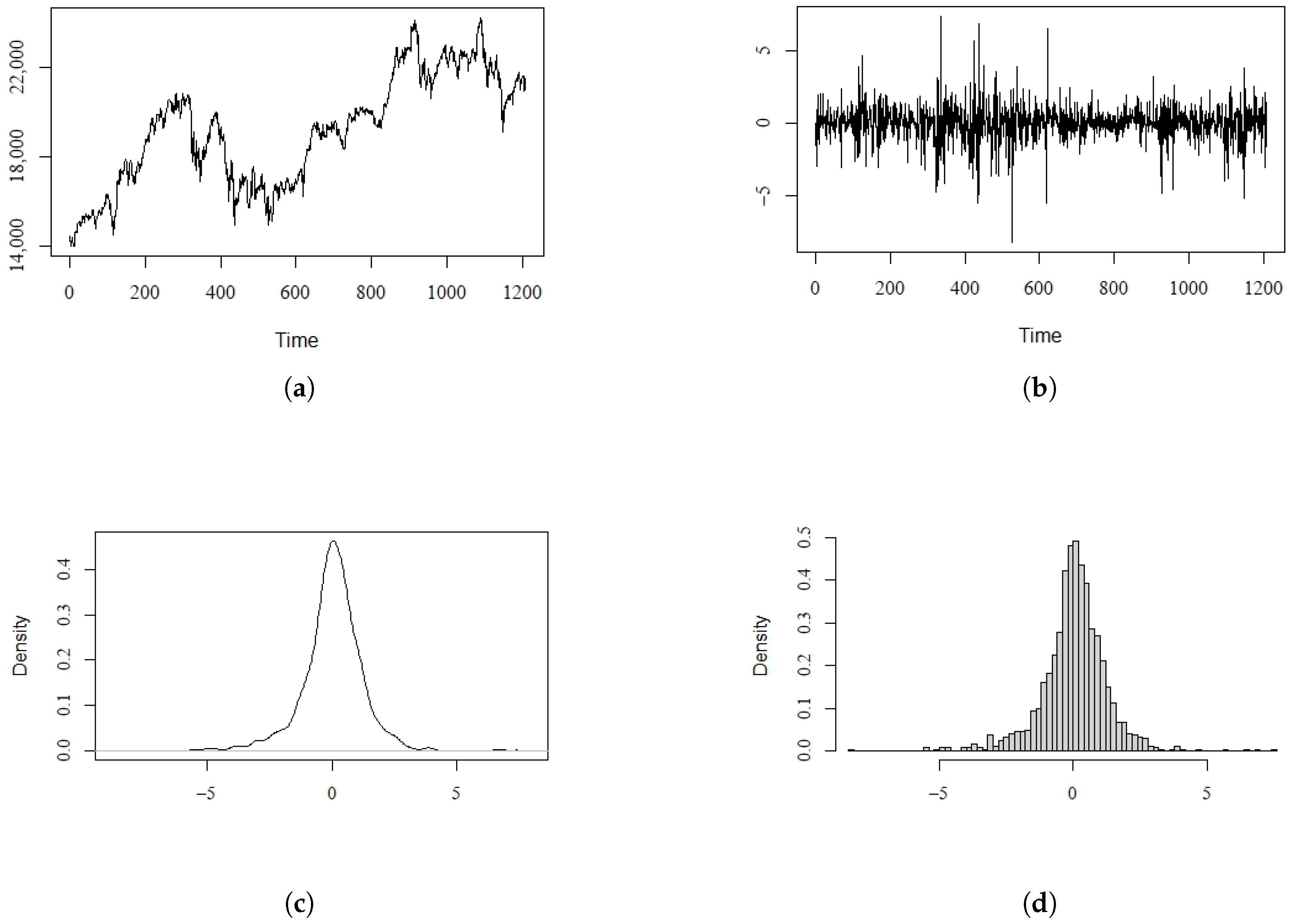
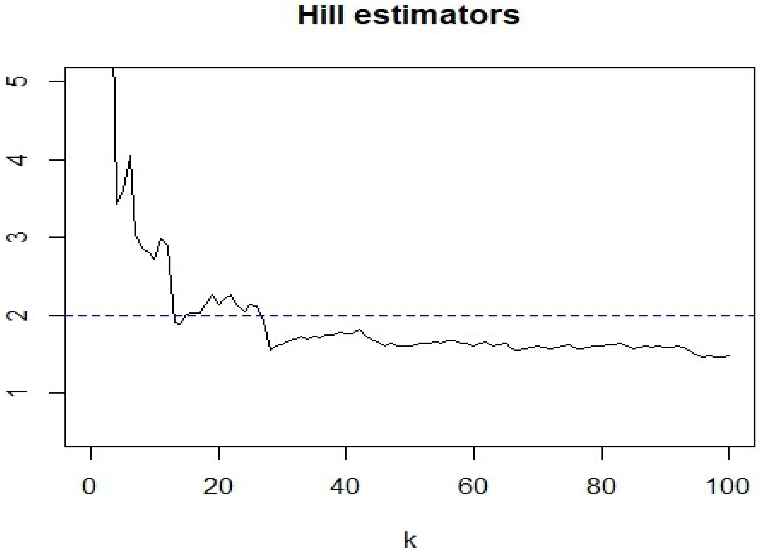
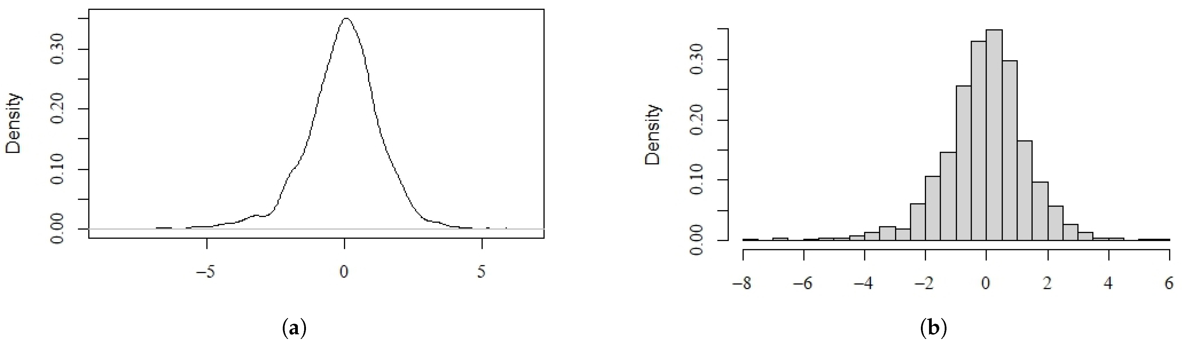
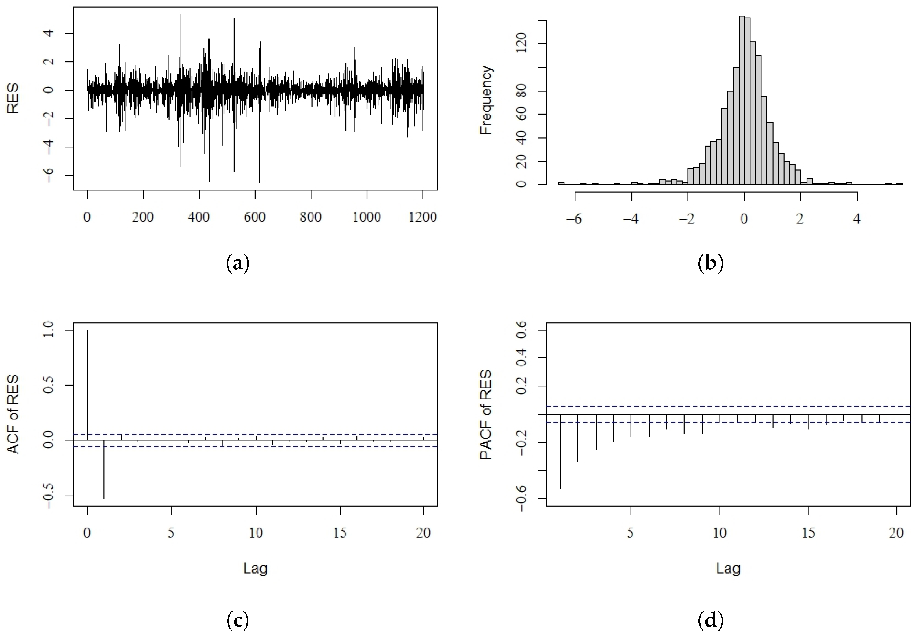
4. Real Data Example

In this section, we provide our analysis of a real data set of the Nikkei 225 in the Japanese stock market. The original data express the closing price on each trading day from 1 May 2014 to 1 April 2019, and there are 1208 valid observations. The explanatory variable is the corresponding daily volume ( z t ). Figure 1a presents the the original data of the closing price on each trading day, which we denote as p t . Figure 1b shows the rescaled 100 times log return, which we denote as { y t } t = 1 1207 : y t = 100 · l o g p t + 1 p t .
Figure 1c,d present the density plots and the histogram of the log return, respectively. From these two nonparametric plots, we can see that the log return data exhibit the characteristics of non-normality and fat tails.
In order to estimate the tail index of { y t 2 } , we use the Hill’s estimator as follows:
H ^ ( k ) = { 1 k i = 1 k [ l o g y ^ n i 2 l o g y ^ n k 2 ] } 1 ,
where k = 1 , 2 , , 100 , and y ^ i 2 is the ith order statistic of { y t 2 } . From Figure 2, we can clearly see that when k > 40 , 1 < H ^ ( k ) < 2 . Thus, the tail index of { y t 2 } lies between 1 and 2, which means E y t 4 = . Since this result does not satisfy the assumption of the asymptotic normality of QMLE, we use the QMELE to estimate the model parameters. First, we need to determine d and locate the threshold parameter r. Following several studies that analyze the stock return series (Chen et al., 2006 [18]; Yang and Chang, 2008 [19]; Chen et al. 2016 [22]), we believe that d = 1 is an appropriate choice. By using the SGS method, we obtain r ^ = 0.0151 and the fitted model
y t = ϕ t ( 1 ) y t 1 + η t 0.0086 + 0.1210 · ϵ t 1 2 + 0.7928 · h t 1 , y t d 0.0151 , ( 0.0145 ) ( 0.0217 ) ( 0.0449 ) ϕ t ( 2 ) y t 1 + η t 0.000113 + 0.0115 · ϵ t 1 2 + 0.8302 · h t 1 , y t d > 0.0151 , ( 0.009829 ) ( 0.0151 ) ( 0.0351 )
ϕ t ( 1 ) = 17.2753 · y t 1 0.4812 · z t , ( 5.8739 ) ( 0.0001387 ) ϕ t ( 2 ) = 1.8262 · y t 1 2.1476 · z t , ( 0.5202 ) ( 0.0006448 )
where the standard errors are given in parentheses. The estimated value of E | η ^ t | is 1.0238, which is very close to 1. Figure 3 shows the density histogram and density plots of η ^ t . We can see that the distribution of η ^ t is asymmetric and heavy tailed and very similar to a double exponential distribution. This evidence determines the choice of using QMELE to fit these Nikkei 225 log return data. Figure 4 shows the diagnostic checking plots for our fitted model. The estimated residuals indicate that the series is stationary. In addition, the histogram plot implies that the standardized residuals are approximately normal, which reveals that our fitted model is suitable. As a comparison, we present the DT-GARCH fitted model of the same data, which is as follows:
y t = 0.1551 y t 1 + ϵ t , y t 1 0.0151 , ( 0.0581 ) 0.0749 y t 1 + ϵ t , y t 1 > 0.0151 , ( 0.0422 ) ϵ t = η t h t ,
h t = 0.1008 + 1264 ϵ t 1 2 + 0.7702 h t 1 , y t 1 0.0151 , ( 0.0169 ) ( 0.0239 ) ( 0.0498 ) 0.0135 + 0.0114 ϵ t 1 2 + 0.8059 h t 1 , y t 1 > 0.0151 , ( 0.0106 ) ( 0.0148 ) ( 0.0321 )
Table 3 displays the AIC of these two fitted models, from which we can see that the AIC of the TVCDT-GARCH model is smaller than the one of the DT-GARCH model.
In conclusion, the real data application reveals that the TVCDT-GARCH model is better than the DT-GARCH model, and the QMELE is proper, compatible, and more accurate than the traditional QMLE. This is not surprising, so in the TVCDT-GARCH model, we consider the influence of the explanatory variable (daily volume). Thus, the model contains more information and can fit the real data better than the DT-GARCH model. Futhermore, the distribution of η t exhibits asymmetric and heavy-tailed features, which is a frequent phenomenon involving financial time series, so we think that using QMELE in parameter-estimation procedures is a pragmatic alternative for practitioners.

5. Conclusions

In this article, we studied the use of the quasi-maximum exponential likelihood estimators (QMELE) to fit the TVCDT-GARCH model. We presented the consistency and the asymptotic normality of the QMELE for the model parameters. The simulation study provided the performance of these estimators. The application of the Nikkei 225 log return series revealed that the TVCDT-GARCH model is appropriate and feasible for analyzing the data, and QMELE provides researchers with a better approach than traditional QMLEs. For further study, the explanatory variables may be developed to higher dimensions, and the models may involve multiple threshold parameters under certain circumstances. These discussions will help us to extend our research in the future.

Author Contributions

Conceptualization, T.Z., L.F., D.W. and Z.Y.; methodology, T.Z. and D.W.; software, T.Z.; validation, T.Z., L.F., D.W. and Z.Y.; formal analysis, T.Z., L.F., D.W. and Z.Y.; investigation, T.Z., L.F., D.W. and Z.Y.; resources, L.F. and D.W.; data curation, T.Z. and D.W.; writing—original draft preparation, T.Z.; writing—review and editing, T.Z., L.F., D.W. and Z.Y.; visualization, T.Z.; supervision, L.F. and D.W.; project administration, L.F., D.W. and Z.Y.; funding acquisition, D.W. All authors have read and agreed to the published version of the manuscript.

Funding

This work is supported by the National Natural Science Foundation of China (No. 12271231, 12001229, 11901053), the National Social Science Foundation of China (No. 21BTJ043, No. 20BTJ056), and the Social Science Foundation of Liaoning Province (No. L22ZD065).

Data Availability Statement

Data are available on the website: hk.finance.yahoo.com, accessed on 1 January 2023.

Acknowledgments

We gratefully acknowledge the anonymous reviewers and editors for their insightful comments on and suggestions for this paper.

Conflicts of Interest

The authors declare no conflict of interest.

Abbreviations

The following abbreviations are used in this manuscript:
ACFAutocorrelation Function Plot
PACFPartial Autocorrelation Function Plot

Appendix A

We need Lemma A1 and Lemma A2 for our proofs; hence, we list two lemmas below.
Lemma A1.
Let ξ p t = 1 + i = 0 ρ i | y t i | , where ρ ( 0 , 1 ) . If Assumptions (1)–(4) hold, then there exist constants C and ρ ( 0 , 1 ) such that the following holds uniformly in Θ:
( 1 ) sup Θ | ϵ t 1 ( γ ) | C ξ p t 1 , sup Θ | | ϵ t ( γ ) γ | | C ξ p t 1 , a n d sup Θ | | 2 ϵ t ( γ ) γ γ | | C ξ p t 1 ;
( 2 ) sup Θ h t ( θ ) C ξ p t 1 ;
( 3 ) sup Θ | | 1 h t ( θ ) h t ( θ ) δ | | C ξ p t 1 ;
( 4 ) sup Θ | | 1 h t ( θ ) h t ( θ ) γ | | C ξ p t 1 .
Lemma A2.
For any θ * Θ , let B η ( θ * ) = { θ Θ : θ θ * < η } be an open neighborhood of θ * with radius η > 0 . If Assumptions (1)–(4) hold, then we have the following:
(a) E [ sup θ Θ l t ( θ ) ] < ;
(b) E [ l t ( θ ) ] has an unique minimum at θ 0 ;
(c) E [ sup θ B η ( θ * ) | l t ( θ ) l t ( θ * ) | ] 0 as η 0 .
Lemma A1 is taken from Lemma A2 in [45] and Lemma A1 of [36]. Lemma 1 is straightforward and follows from the central limit theorem for a martingale difference sequence. For Lemma 2, by letting ω t 1 in Lemmas 2.2 and 2.3 of [36], we can directly obtain Lemma 2.2. The detailed proofs of Lemma A2, Lemma 3, Theorem 1 and Theorem 2 can be found in the appendix of [41], and, hence, we omit the proofs of these lemmas and theorems.

References

  1. Nicholls, D.F.; Quinn, B.G. Random Coefficient Autoregressive Models: An Introduction; Springer: New York, NY, USA, 1982. [Google Scholar]
  2. Tjostheim, D. Estimation in nonlinear time series models. Stoch. Process. Their Appl. 1986, 21, 251–273. [Google Scholar] [CrossRef]
  3. Kim, Y.W.; Basawa, I.V. Empirical Bayes estimation for first order autoregressive processes. Aust. J. Stat. 1992, 34, 105–114. [Google Scholar] [CrossRef]
  4. Hwang, S.Y.; Basawa, I.V. Asymptotic optimal inference for a class of nonlinear time series models. Stoch. Process. Their Appl. 1993, 46, 91–113. [Google Scholar] [CrossRef]
  5. Hwang, S.Y.; Basawa, I.V. Large sample inference for conditional exponential families with applications to nonlinear time series. J. Stat. Plan. Inference 1994, 38, 141–157. [Google Scholar] [CrossRef]
  6. Hwang, S.Y.; Basawa, I.V. Parameter estimation for generalized random coefficient autoregressive processes. J. Stat. Plan. Inference 1998, 68, 323–337. [Google Scholar] [CrossRef]
  7. Aue, A. Strong approximation for RCA(1) time series with applications. Stat. Probab. Lett. 2004, 68, 369–382. [Google Scholar] [CrossRef]
  8. Aue, A.; Horvath, L.; Steinebach, J. Estimation in Random Coefficient Autoregressive Models. J. Time Ser. Anal. 2006, 27, 61–76. [Google Scholar] [CrossRef]
  9. Thavaneswaran, A.; Appadoo, S.S.; Ghahramani, M. RCA models with GARCH innovations. Appl. Math. Lett. 2009, 22, 110–114. [Google Scholar] [CrossRef]
  10. Tong, H. On a Threshold Model; Sijhoff & Noordhoff: Amsterdam, The Netherlands, 1978. [Google Scholar]
  11. Tong, H.; Lim, K.S. Threshold autoregression, limit cycles and cyclical data. J. R. Stat. Soc. Ser. B (Methodol.) 1980, 42, 245–268. [Google Scholar] [CrossRef]
  12. Engle, R.F. Autoregressive Conditional Heteroscedasticity with Estimates of the Variance of United Kingdom Inflation. Econometrica 1982, 50, 987–1007. [Google Scholar] [CrossRef]
  13. Bollerslev, T. Generalized autoregressive conditional heteroskedasticity. J. Econom. 1986, 31, 307–327. [Google Scholar] [CrossRef]
  14. Karpoff, J.M. The Relation between Price Changes and Trading Volume: A Survey. J. Financ. Quant. Anal. 1987, 22, 109–126. [Google Scholar] [CrossRef]
  15. Tong, H. Non-Linear Time Series: A Dynamical System Approach; Oxford University Press: Oxford, UK, 1990. [Google Scholar]
  16. Li, C.W.; Li, W.K. On a Double-Threshold Autoregressive Heteroscedastic Time Series Model. J. Appl. Econometr. 1996, 11, 253–274. [Google Scholar] [CrossRef]
  17. Brooks, C. A Double-threshold GARCH Model for the French Franc/Deutschmark exchange rate. J. Forecast. 2001, 20, 135–143. [Google Scholar] [CrossRef]
  18. Chen, C.W.S.; Yang, M.J.; Gerlach, R.; Jim, L.H. The asymmetric reactions of mean and volatility of stock returns to domestic and international information based on a four-regime double-threshold GARCH model. Phys. Stat. Mech. Appl. 2006, 366, 401–418. [Google Scholar] [CrossRef]
  19. Yang, Y.L.; Chang, C.L. A double-threshold GARCH model of stock market and currency shocks on stock returns. Math. Comput. Simul. 2008, 79, 458–474. [Google Scholar] [CrossRef]
  20. Chen, C.W.S.; Gerlach, R. Semi-parametric quantile estimation for double threshold autoregressive models with heteroskedasticity. Comput. Stat. 2013, 28, 1103–1131. [Google Scholar] [CrossRef]
  21. Chen, C.W.S.; Chen, M.; Chen, H. Pairs Trading via Three-Regime Threshold Autoregressive GARCH Models. In Proceedings of the 7th International Conference of the Thailand Econometric Society, TES 2014, Chiang Mai, Thailand, 8–10 January 2014; pp. 127–140. [Google Scholar]
  22. Chen, C.W.S.; So, M.K.P.; Chiang, T.C. Evidence of Stock Returns and Abnormal Trading Volume: A Threshold Quantile Regression Approach. Jpn. Econ. Rev. 2016, 67, 96–124. [Google Scholar] [CrossRef]
  23. Luukkonen, R.; Saikkonen, P.; Teräsvirta, T. Testing linearity against smooth transition autoregressive models. Biometrika 1988, 75, 491–499. [Google Scholar] [CrossRef]
  24. Teräsvirta, T. Specification, estimation, and evaluation of smooth transition autoregressive models. J. Am. Stat. Assoc. 1994, 89, 208–218. [Google Scholar]
  25. Zheng, H.T.; Basawa, I.V. First-order observation-driven integer-valued autoregressive processes. Stat. Probab. Lett. 2008, 78, 1–9. [Google Scholar] [CrossRef]
  26. Yu, M.J.; Wang, D.H.; Yang, K. A class of observation-driven random coefficient INAR(1) processes based on negative binomial thinning. J. Korean Stat. Soc. 2019, 48, 248–264. [Google Scholar] [CrossRef]
  27. Yang, K.; Li, H.; Wang, D.H.; Zhang, C.H. Random coefficients integer-valued threshold autoregressive processes driven by logistic regression. AStA Adv. Stat. Anal. 2021, 105, 533–557. [Google Scholar] [CrossRef]
  28. Hwang, S.Y.; Basawa, I.V. Explosive Random Coefficient AR(1) Processes and Related Asymptotics for Least Squares Estimation. J. Time Ser. Anal. 2005, 26, 807–824. [Google Scholar] [CrossRef]
  29. Berkes, I.; Horvath, L.; Ling, S.Q. Estimation in nonstationary random coefficient autoregressive models. J. Time Ser. Anal. 2009, 30, 395–416. [Google Scholar] [CrossRef]
  30. Aue, A.; Horvath, L. Quasi-likelihood estimation in stationary and nonstationary autoregressive models with random coefficients. Stat. Sin. 2011, 21, 973–999. [Google Scholar]
  31. Weiss, A. Asymptotic theory for ARCH models: Estimation and testing. Econom. Theory 1986, 2, 107–131. [Google Scholar] [CrossRef]
  32. Engle, R.F.; Bollerslev, T. Modelling the persistence of conditional variances. Econom. Rev. 1986, 5, 1–50. [Google Scholar] [CrossRef]
  33. Berkes, I.; Horvath, L.; Kokoszka, P. GARCH processes: Structure and estimation. Bernoulli 2003, 9, 201–227. [Google Scholar] [CrossRef]
  34. Francq, C.; Zokaian, J.M. Maximum Likelihood Estimation of Pure GARCH and ARMA-GARCH Processes. Bernoulli 2004, 10, 605–637. [Google Scholar] [CrossRef]
  35. Hall, P.; Yao, Q. Inference in ARCH and GARCH models with heavy-tailed errors. Econometrica 2003, 71, 285–317. [Google Scholar] [CrossRef]
  36. Zhu, K.; Ling, S.Q. Global self-weighted and local quasi-maximum exponential likelihood estimators for ARMA-GARCH/IGARCH models. Ann. Stat. 2011, 39, 2131–2163. [Google Scholar] [CrossRef]
  37. Tsay, R.S. Testing and modeling threshold autoregressive processes. J. Am. Stat. Assoc. 1989, 84, 231–240. [Google Scholar] [CrossRef]
  38. Li, D.; Ling, S.Q. On the least squares estimation of multiple-regime threshold autoregressive models. J. Econom. 2012, 167, 240–253. [Google Scholar] [CrossRef]
  39. Yu, P. Likelihood estimation and inference in threshold regression. J. Econom. 2012, 167, 274–294. [Google Scholar] [CrossRef]
  40. Li, D.; Tong, H. Nested sub-sample search algorithm for estimation of threshold models. Stat. Sin. 2016, 26, 1543–1554. [Google Scholar] [CrossRef]
  41. Zhang, T.W.; Wang, D.H.; Yang, K. Quasi-maximum exponential likelihood estimation for double-threshold GARCH models. Can. J. Stat. 2021, 49, 1152–1178. [Google Scholar] [CrossRef]
  42. Sheng, D.S.; Wang, D.H.; Kang, Y. A new RCAR(1) model based on explanatory variables and observations. Commun. Stat.-Theory Methods 2022. [Google Scholar] [CrossRef]
  43. Li, G.D.; Guan, B.; Li, W.K.; Yu, P.L.H. Hysteretic autoregressive time series models. Biometrika 2015, 102, 717–723. [Google Scholar] [CrossRef]
  44. Silverman, B.W. Density Estimation for Statistics and Data Analysis; Chapman and Hall: New York, NY, USA, 1986. [Google Scholar]
  45. Ling, S.Q. Self-weighted and local quasi-maximum likelihood estimators for ARMA-GARCH/IGARCH models. J. Econom. 2007, 140, 849–873. [Google Scholar] [CrossRef]
Figure 1. The data of the Nikkei 225. (a) Original closing price. (b) 100 times log return. (c) Density plots of log return. (d) Frequency histogram of log return.
Axioms 12 00476 g001
Figure 2. The Hill’s estimators of y t 2 .
Axioms 12 00476 g002
Figure 3. The frequency histogram and density plots of η ^ t . (a) Density plots. (b) Frequency histogram.
Axioms 12 00476 g003
Figure 4. Diagnostic checking plots for the Nikkei 225 (log return) data. (a) Standardized residuals; (b) histogram of standardized residuals; (c) ACF plot of residuals; (d) PACF plot of residuals.
Axioms 12 00476 g004
Table 1. Estimation performance results of D G P 1 (QMELE vs. standard QMLE ).
Parameters c 11 ω 1 α 11 β 11 c 21 ω 2 α 21 β 21 r c 11 ω 1 α 11 β 11 c 21 ω 2 α 21 β 21 r
nTrue Value0.80.30.20.40.30.10.30.51 0.80.30.20.40.30.10.30.51
QMELE Standard QMLE
η t N ( 0 , π 2 )
300Bias0.10070.04810.0039−0.0457−0.02360.0365−0.0077−0.01840.0210 −0.01830.18700.10130.0089−0.02630.08280.1431−0.0126−0.1083
SD0.41950.16910.12110.23410.15840.18790.12310.18770.1306 0.32060.20720.15710.19660.11390.25330.16430.17170.1589
ASD0.76500.15170.14010.18950.24460.16210.10200.1707 0.26970.19190.12780.16540.05880.22410.14360.1638
600Bias0.05860.03950.0152−0.0461−0.01470.0258−0.0075−0.01360.0294 −0.04080.16810.10190.0171−0.01340.07280.1464−0.0036−0.1193
SD0.28600.12200.07840.14540.09550.11990.08370.10930.1049 0.26730.15230.11850.14240.07910.15880.10680.10610.1491
ASD0.49600.10080.06820.12890.11120.10260.07330.1144 0.19530.14200.09650.12580.04070.14160.10340.1098
900Bias0.05640.03280.0153−0.0403−0.00390.0219−0.0008−0.01760.0177 −0.06000.16510.10130.0205−0.01030.06790.14440.0036−0.1163
SD0.24560.11350.06650.12010.07500.09330.06260.08640.0945 0.18400.14050.09160.11320.06940.11390.08670.07980.1219
ASD0.43460.08930.06360.11300.07980.07640.05960.0893 0.15690.12290.08210.10500.03450.10810.08380.0867
η t L a p l a c e ( 0 , 1 )
300Bias0.08790.03150.0132−0.00710.00270.0324−0.01200.-00290.0238 −0.14110.26650.19330.0543−0.00940.13660.2501−0.0133-0.2345
SD0.42550.32100.14800.28140.24190.18180.13220.16760.1953 0.37700.32460.28380.26250.14090.28430.24670.16240.2522
ASD0.91720.24650.14070.24240.16720.15600.10860.1498 0.43440.31310.23610.19980.09050.26970.19770.1553
600Bias0.02660.01690.03790.00370.00440.0171−0.0085−0.00250.0140 −0.15100.27460.18520.0438−0.00500.12840.2671−0.0070−0.2326
SD0.34770.16250.12540.22690.11970.09230.07900.09230.1361 0.26980.28850.26090.19270.10190.17690.17810.10630.2089
ASD0.79760.17440.14170.18690.12230.08030.07540.0923 0.42360.32020.59720.17110.06770.16640.15240.1054
900Bias0.05030.01340.01310.00070.00170.0142−0.0017−0.00730.0145 −0.17300.27290.18610.03880.00400.11630.2783−0.0051−0.2459
SD0.30700.13060.11450.17610.08930.06840.06310.06740.1015 0.23590.23000.19480.16920.08560.13080.13710.07980.1986
ASD0.49790.12860.09850.14580.08540.05740.06160.0719 0.29800.24280.18460.16430.05510.11980.12610.0810
η t ( π 2 3 ) t 3
300Bias0.04600.02540.03610.00620.00940.0353−0.0110−0.01750.0181 −0.20240.28280.21060.12210.01820.15520.3058−0.0198-0.2972
SD0.38740.27620.23360.31340.16960.17850.15160.18370.1897 0.54920.54340.46230.38840.36930.36810.40190.19900.4593
ASD0.98680.26490.34770.26150.23220.15260.12040.1602 0.56550.42920.33560.23990.14690.35800.27900.1928
600Bias0.07440.02210.0321−0.00300.00760.01970.0061−0.00950.0157 −0.22570.30670.21340.11140.01390.16500.3656−0.0168−0.3080
SD0.31700.17610.20350.25390.13370.09530.09710.10080.1807 0.39580.38140.42690.38020.22850.27140.38760.14160.3693
ASD0.72930.22120.18500.21290.15350.07960.08870.1002 0.54300.44990.36540.25850.16190.23690.24510.1423
900Bias0.05200.02060.0228−0.00160.00170.01290.0004−0.00940.0061 −0.22300.28760.23410.10720.01710.15150.3606−0.0065−0.2269
SD0.29630.15920.18570.19340.11090.06950.07520.07560.1606 0.37030.36290.39250.29760.17300.19370.33820.12240.3537
ASD0.66930.18320.15870.18250.09650.05580.07320.0921 0.53290.37520.35680.24860.11120.17980.21850.1162
Table 2. Estimation performance results of D G P 2 (QMELE vs. Standard QMLE ).
Parameters c 11 d 1 ω 1 α 11 β 11 c 21 d 2 ω 2 α 21 β 21 r c 11 d 1 ω 1 α 11 β 11 c 21 d 2 ω 2 α 21 β 21 r
nTrue Value0.70.20.10.50.30.30.50.10.20.60 0.70.20.10.50.30.30.50.10.20.60
QMELE Standard QMLE
η t N ( 0 , π 2 )
300Bias0.0359−0.01370.0481−0.03280.0155−0.00960.03200.0422−0.0195−0.0178−0.0383 −0.0959−0.09170.12590.22740.0363−0.0223−0.01260.18000.07830.0138−0.2076
SD0.54090.53060.08470.23380.14850.20100.38380.11250.09260.13540.3876 0.27590.29870.11850.22730.14750.11710.24920.16770.12130.12960.3679
ASD1.42291.12410.19530.15000.20430.18470.50380.07680.09080.1192 0.31050.37800.39150.23900.20670.06210.16510.10510.11720.1092
600Bias0.0198−0.00960.0458−0.01160.0102−0.00060.01460.0295−0.0191−0.0035−0.0181 −0.1068−0.06560.11970.21450.0495−0.0100−0.01670.15220.00970.0237−0.1926
SD0.28240.30300.09400.14760.14510.10570.25270.07000.06670.08180.3152 0.18870.20990.08200.17820.10740.07690.16000.10490.09720.08450.2622
ASD0.56580.58570.07700.11480.13350.17990.32720.05260.06380.0826 0.20920.27390.13850.15600.12550.03890.11550.07060.08330.0748
900Bias0.0046−0.01090.0426−0.01870.01850.00590.01530.0198−0.01660.00190.0009 −0.1023−0.06850.12420.20120.0554−0.0090−0.01880.14480.09120.0307−0.1842
SD0.30390.25150.06480.19710.10640.13430.23730.05420.05510.06740.2467 0.16930.16910.08240.14520.10050.05930.13320.08480.08340.06760.2431
ASD0.66370.53100.05520.09060.09160.20170.25950.04210.05240.0671 0.17560.18830.10450.12910.10110.03290.09820.05740.06810.0608
η t L a p l a c e ( 0 , 1 )
300Bias0.0313−0.01200.04860.00560.01910.00140.02380.0368−0.0076−0.0164−0.0621 −0.1206−0.17710.19240.40320.05850.0047−0.06410.27740.15120.0214−0.3335
SD0.31930.38970.10950.26400.20000.11720.27730.11650.10370.12240.4687 0.43130.45470.25270.49250.21870.17160.39330.25750.19040.15130.5577
ASD1.32261.58660.37960.26240.38780.15250.43860.08340.10690.1185 1.16421.11361.25070.51340.41340.12860.33950.16320.18040.1230
600Bias0.0017−0.02260.05140.01350.01350.00020.01540.0266-0.0064-0.0123−0.0289 −0.1515−0.16250.19360.38080.06360.0094−0.06310.24440.18410.01000.4300
SD0.32270.38900.10520.21810.13350.07160.23010.07230.07050.08050.3505 0.33110.37390.16990.35820.20840.11880.34810.16620.16640.09780.4905
ASD0.85160.91700.19920.18110.23170.08310.28780.05700.07530.0816 0.68770.93541.03920.48910.60410.12110.25330.11250.13320.0848
900Bias0.0030−0.00690.05040.00610.01730.00560.02150.0192−0.0101−0.0014−0.0393 −0.1409−0.15520.19970.36130.07400.0146−0.05300.22730.19800.0318−0.3594
SD0.24280.27480.08460.19180.13050.08690.18850.05500.05930.06230.3283 0.34400.32440.17040.29860.16440.15520.32820.12900.14590.08340.4708
ASD0.59470.63940.14590.16830.18940.10040.29740.04520.05920.0651 0.83451.03950.86020.37040.26560.08640.22900.09150.11070.0691
η t ( π 2 3 ) t 3
300Bias0.0433−0.00230.06260.02290.00300.01540.01120.0438−0.0093−0.0229−0.0537 −0.1922−0.22680.24130.44130.08250.0270−0.08130.33280.19050.0208−0.3948
SD0.37660.37970.14790.32300.22280.29490.30530.12840.11310.13620.4103 0.56780.63240.30590.63100.29670.25490.54790.39340.32450.19240.7518
ASD1.68081.38410.39480.31330.47110.15280.42420.09210.12360.1341 2.11213.53924.83411.20460.69660.30200.73810.28890.31470.1813
600Bias0.0107−0.01940.05500.01150.02760.0079−0.01950.0282−0.0095-0.0107-0.0467 -0.1745-0.21910.24230.45050.08550.0376-0.13910.30910.23090.0266-0.4178
SD0.30620.59620.18081.30400.19330.10420.43180.08650.08500.09480.4613 0.40700.51250.36490.60250.26150.24360.51460.32190.29680.14200.6121
ASD0.74850.86550.39990.27820.21640.12420.44060.06380.08790.0947 1.97902.86214.01551.31840.77230.53500.82050.28760.29600.1757
900Bias0.0111-0.01580.05440.01210.02800.01240.00820.0208-0.0076-0.0082-0.0466 -0.1752-0.19760.22170.40250.09380.0281-0.12990.30510.25090.0400-0.3946
SD0.30030.35180.15120.26890.18550.15210.26430.06340.07070.07190.3832 0.33320.43590.24500.44160.20840.18440.42310.30720.28670.12720.5482
ASD0.80890.87410.19640.23150.17940.12360.34300.05110.07190.0767 1.40531.89314.52130.91270.52230.20290.46960.19300.22970.1177
Table 3. AIC of two fitted models.
TVCDT-GARCHDT-GARCH
AIC1922.5221925.186
Disclaimer/Publisher’s Note: The statements, opinions and data contained in all publications are solely those of the individual author(s) and contributor(s) and not of MDPI and/or the editor(s). MDPI and/or the editor(s) disclaim responsibility for any injury to people or property resulting from any ideas, methods, instructions or products referred to in the content.

