Article

A New Probability Distribution: Model, Theory and Analyzing the Recovery Time Data

by
Huda M. Alshanbari
1,
Omalsad Hamood Odhah
1,
Zubair Ahmad
2,*,
Faridoon Khan
3 and
Abd Al-Aziz Hosni El-Bagoury
4
1
Department of Mathematical Sciences, College of Science, Princess Nourah bint Abdulrahman University, P.O. Box 84428, Riyadh 11671, Saudi Arabia
2
Department of Statistics, Quaid-i-Azam University, Islamabad 44000, Pakistan
3
Pakistan Institute of Development Economics, Islamabad 44000, Pakistan
4
Basic Sciences Department, Higher Institute of Engineering and Technology, El-Mahala El-Kobra 31951, Egypt
*
Author to whom correspondence should be addressed.
Axioms 2023, 12(5), 477; https://doi.org/10.3390/axioms12050477
Submission received: 3 March 2023 / Revised: 30 April 2023 / Accepted: 8 May 2023 / Published: 15 May 2023

Abstract

:
Probability models are frequently used in numerous healthcare, sports, and policy studies. These probability models use datasets to identify patterns, analyze lifetime scenarios, predict outcomes of interest, etc. Therefore, numerous probability models have been studied, introduced, and implemented. In this paper, we also propose a novel probability model for analyzing data in different sectors, particularly in biomedical and sports sciences. The probability model is called a new modified exponential-Weibull distribution. The heavy-tailed characteristics along with some other mathematical properties are derived. Furthermore, the estimators of the new modified exponential-Weibull are derived. A simulation study of the new modified exponential-Weibull model is also provided. To illustrate the new modified exponential-Weibull model, a practical dataset is analyzed. The dataset consists of seventy-eight observations and represents the recovery time after the injuries in different basketball matches.

1. Introduction

The development and introduction of novel statistical methodologies is an interesting area of research [1]. Numerous statistical models have been extended and proposed for data modeling in different sectors. For example, (i) Ref. [2] implemented statistical models in the epidemiology sector, (ii) Ref. [3] used the Weibull model for data modeling in the energy sector, (iii) Refs. [4,5] used the Gumbel distribution in the hydrological sector, (iv) Ref. [6] implemented a new version of the Lomax model in the engineering and medical sectors, (v) Ref. [7] introduced an updated form of the Pareto distribution distribution for analyzing the fire insurance dataset, (vi) Ref. [8] used the inverse Rayleigh model in the industrial sector, (vii) Ref. [9] applied the Gamma distribution in the engineering sector, (viii) Ref. [10] applied the uniform distribution in chemical engineering, (ix) Ref. [11] implemented the uniform distribution in the material sciences, and (x) Ref. [12] applied a new version of the logistic model in the actuarial sciences, among others.
Among the above sectors, the statistical distributions have wider applications in the medical, sports, and other related sectors. For example, (i) Ref. [13] used an updated form of the inverse Weibull model for analyzing a breast cancer dataset, (ii) Ref. [14] used the odd Weibull inverse Topp–Leone model for analyzing COVID-19 data, (iii) Ref. [15] introduced a novel statistical model for analyzing COVID-19 data in China, (iv) Ref. [16] provided a comparison of different statistical models for leukemia data, (v) Ref. [17] used a new alpha power Weibull model for analyzing the waiting time till the first goal in different football matches, and (vi) Ref. [18] implemented a double Poisson model to predict football results.
Among the abovementioned statistical/probability models, the Weibull distribution holds a special place [19]. The Weibull distribution has been implemented by many researchers for data modeling in different fields. For example, (i) Ref. [20] used the Weibull distribution to describe precipitation; (ii) Ref. [21] used the q-Weibull distribution for analyzing dielectric breakdown data (for more applicabilities of the q-Weibull distribution, we refer to [22,23,24]; (iii) Ref. [25] found that the Weibull distribution is one of the most popular distributions to describe wind speed; and (iv) Ref. [26] introduced a system of distributions that generalize the exponential and Weibull distributions suitable for hydroclimatic variables.
Let T x ; Λ be the CDF of the Weibull random variable, say X, with ϕ 1 (shape parameter) and ϕ 2 (scale parameter). Then, the CDF of X T x ; Λ , is given by
T x ; Λ = 1 e ϕ 2 x ϕ 1 , x 0 , ϕ 1 , ϕ 2 > 0 ,
where Λ = ϕ 1 , ϕ 2 .
Corresponding to T x ; Λ , the PDF t x ; Λ and hazard function (HF) h x ; Λ of the Weibull model are given by
t x ; Λ = ϕ 1 ϕ 2 x ϕ 1 1 e ϕ 2 x ϕ 1 , x , ϕ 1 , ϕ 2 > 0 ,
and
h x ; Λ = ϕ 1 ϕ 2 x ϕ 1 1 , x , ϕ 1 , ϕ 2 > 0 ,
respectively.
From h x ; Λ of the Weibull model in Equation (2), it is obvious that h x ; Λ has three possible shapes, including
  • Increasing, if ϕ 1 > 1 ;
  • Decreasing, if ϕ 1 < 1 ;
  • Constant, if ϕ 1 = 1 .
From Equation (2), it is obvious that the Weibull distribution has three possible shapes. To improve the characteristics of the Weibull model, numerous statistical methodologies have been proposed. For example, Ref. [27] proposed the logarithmic-U (Log-U) method. The CDF F x ; δ , λ , Λ of the Log-U family is
F x ; δ , λ , Λ = 1 1 λ U x ; Λ λ log U x ; Λ δ , x R ,
where δ R + , λ R + , Λ is a parameter vector, and U x ; Λ represents the CDF of the baseline model associated with the Log-U family of distributions.
Ref. [28] suggested another approach, called a new modified-G (for short “NM-G”) family. The CDF F x ; κ , Λ of the NM-G family is
F x ; κ , Λ = G x ; Λ κ κ 1 + G x ; Λ , x R ,
where κ 1 , κ 1 , and G x ; Λ is the CDF of the baseline distribution associated with the NM-G family of distributions.
Another useful approach for updating the characteristics of the statistical models is called a new modified exponential-X (NME-X) family [29]. The CDF F x ; α , Λ of the NME-X family is
F x ; α , Λ = 1 α 2 T ¯ x ; Λ α + T x ; Λ 2 , x R ,
where α > 0 , T ¯ x ; Λ = 1 T x ; Λ , and T x ; Λ is the CDF of the baseline distribution associated with the NME-X family.
The PDF f x ; α , Λ corresponding to Equation (3) is expressed by
F x ; α , Λ = α 2 t x ; Λ α + T x ; Λ 3 α + 2 T x ; Λ ,
where d d x T x ; Λ = t x ; Λ .
Furthermore, corresponding to Equations (3) and (4), the survival function (SF) S x ; α , Λ = 1 F x ; α , Λ and hazard function (HF) h x ; α , Λ = f x ; α , Λ 1 F x ; α , Λ are given, respectively, by
S x ; α , Λ = α 2 T ¯ x ; Λ α + T x ; Λ 2 ,
and
h x ; α , Λ = t x ; Λ T ¯ x ; Λ α + T x ; Λ α + 2 T x ; Λ .
In this paper, we incorporate the NME-X approach to introduce a novel extended version of the Weibull model, called a new modified exponential-Weibull (NME-Weibull) distribution. The NME-Weibull is a more flexible form of the Weibull model. This fact is shown by plotting the shapes of its HF and applying it to a healthcare-related dataset.

2. An NME-Weibull Model

Suppose X has an NME-Weibull model, if CDF F x ; α , Λ is
F x ; α , Λ = 1 α 2 e ϕ 2 x ϕ 1 α + 1 e ϕ 2 x ϕ 1 2 , x 0 .
Corresponding to Equation (6), the PDF f x ; α , Λ of the NME-Weibull model is
f x ; α , Λ = α 2 ϕ 1 ϕ 2 x ϕ 1 1 e ϕ 2 x ϕ 1 α + 1 e ϕ 2 x ϕ 1 3 α + 2 1 e ϕ 2 x ϕ 1 .
Some possible shapes of f x ; α , Λ of the NME-Weibull model are provided in Figure 1. From the plots in Figure 1, we can see that f x ; α , Λ of the NME-Weibull model has four shapes, including (i) decreasing, (ii) positively skewed, (iii) symmetrical, and (iv) negatively skewed.
Furthermore, plots of the SF S x ; α , Λ , HF h x ; α , Λ , and cumulative HF H x ; α , Λ of the NME-Weibull model are given by
S x ; α , Λ = α 2 e ϕ 2 x ϕ 1 α + 1 e ϕ 2 x ϕ 1 2 ,
h x ; α , Λ = ϕ 1 ϕ 2 x ϕ 1 1 α + 1 e ϕ 2 x ϕ 1 α + 2 1 e ϕ 2 x ϕ 1 ,
and
H x ; α , Λ = log α 2 e ϕ 2 x ϕ 1 α + 1 e ϕ 2 x ϕ 1 2 ,
respectively.
Some possible shapes of h x ; α , Λ of the NME-Weibull model are sketched in Figure 2. The plots in Figure 2 reveal that h x ; α , Λ of the NME-Weibull model has four shapes, including (i) decreasing, (ii) unimodal, (iii) modified unimodal, and (iv) increasing.

3. Properties

This section offers different properties of the NME-Weibull model, including the (i) shapes of NME-Weibull PDF and HF, (ii) heavy-tailed (HT) characteristic, (iii) quantile function (QF), (iv) r th mean, and (v) moment generator function (MGF).

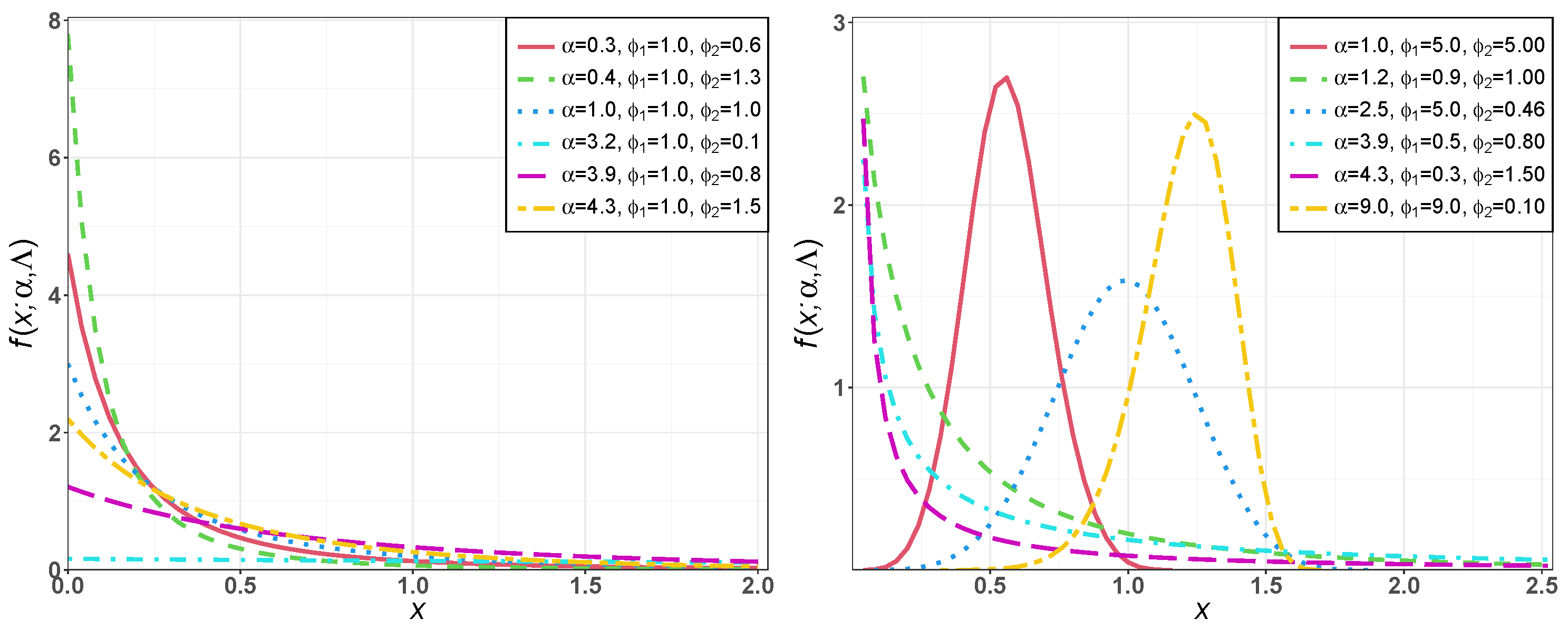
3.1. Shapes of NME-Weibull PDF and HF

The behaviors of the PDF of the NME-Weibull distribution when x 0 and x are, respectively, given by
lim x 0 f x ; α , Λ = if ϕ 1 < 1 , α + 2 α ϕ 2 if ϕ 1 = 1 , 0 if ϕ 1 > 1 ,
lim x f x ; α , Λ = 0 .
This clearly appears in Figure 1.
Similarly, the behaviors of the HF when x 0 and x are, respectively, given by
lim x 0 h x ; α , Λ = if ϕ 1 < 1 , α + 2 α ϕ 2 if ϕ 1 = 1 , 0 if ϕ 1 > 1 ,
lim x h x ; α , Λ = 0 if ϕ 1 < 1 , ϕ 2 if ϕ 1 = 1 , if ϕ 1 > 1 .
This clearly appears in Figure 2.

3.2. The HT Characteristic

The probability distributions that posses the HT property/characteristic are competent for modeling data in applied sciences. The HT distributions are especially very prominent in the financial sectors and extreme value theory [30]. However, there are only a few probability distributions that possess the HT property [31]. Therefore, researchers have been trying to develop new probability distributions that possess the HT property.
Here, we derive the HT characteristic of the NME-Weibull model. The HT probability models possess a very useful characteristic called a regular variation property (RVP). The regularly varying function (RVF) is a function of a real variable that behaves similar to a power law function at infinity (i.e., x ). For more detail, we refer the reader to [32]. According to Karamata’s theorem of [33], using the SF, we have
Theorem 1. 
If T ¯ x ; Λ = 1 T x ; Λ is the SF of the regularly varying probability model, then S x ; α , Λ = 1 F x ; α , Λ is also a regularly varying probability model.
Proof. 
Suppose that lim x T ¯ τ x ; Λ T ¯ x ; Λ = p τ is a finite and nonzero function τ > 0 . Then, using Equation (5), we have
S τ x ; α , Λ S x ; α , Λ = α 2 T ¯ τ x ; Λ α + T τ x ; Λ 2 α 2 T ¯ x ; Λ α + T x ; Λ 2 = α 2 T ¯ τ x ; Λ α + T τ x ; Λ 2 × α + T x ; Λ 2 α 2 T ¯ x ; Λ = α 2 T ¯ τ x ; Λ α 2 T ¯ x ; Λ × α + T x ; Λ 2 α + T τ x ; Λ 2 = T ¯ τ x ; Λ T ¯ x ; Λ × α + T x ; Λ 2 α + T τ x ; Λ 2 .
Then,
lim x S τ x ; α , Λ S x ; α , Λ = lim x T ¯ τ x ; Λ T ¯ x ; Λ × α + T x ; Λ 2 α + T τ x ; Λ 2 lim x = p τ × lim x α + T x ; Λ 2 α + T τ x ; Λ 2 .
Using T x ; Λ = 1 e ϕ 2 x ϕ 1 in Equation (8), we obtain
lim x S τ x ; α , Λ S x ; α , Λ = p τ × lim x α + 1 e ϕ 2 x ϕ 1 2 α + 1 e ϕ 2 ( τ x ) ϕ 1 2 = p τ × α + 1 lim x e ϕ 2 x ϕ 1 2 α + 1 lim x e ϕ 2 ( τ . x ) ϕ 1 2 .
Now, since τ , ϕ 1 , ϕ 2 > 0 , then
lim x e ϕ 2 x ϕ 1 = lim x 1 e ϕ 2 x ϕ 1 = 1 lim x e ϕ 2 x ϕ 1 = 1 e ϕ 2 lim x x ϕ 1 0 ,
and
lim x e ϕ 2 ( τ . x ) ϕ 1 = lim x 1 e ϕ 2 ( τ . x ) ϕ 1 = 1 lim x e ϕ 2 ( τ . x ) ϕ 1 = 1 e ϕ 2 lim x ( τ . x ) ϕ 1 0 .
Thus,
lim x S τ x ; α , Λ S x ; α , Λ = p τ × α + 1 0 2 α + 1 0 2 , = p τ × α + 1 2 α + 1 2 , = p τ .
This function in Equation (9) shows that lim x S τ x ; α , Λ S x ; α , Λ is finite and a nonzero function τ > 0 . Therefore, the function S x ; α , Λ satisfies the RVP. It is important to note that by Karamata’s characterization theorem, the function p has the form p τ = τ σ , where σ R is called the index of regular variation, and τ > 0 .

3.3. The Quantile Function

The quantile function (QF) of the NME-Weibull distribution), say Q ( u ) , where 0 < u < 1 , can be obtained by solving the equation F ( Q ( u ) ) = u in Equation (6) for Q ( u ) in terms of u, and this implies
Q ( u ) = 1 ϕ 2 log 2 ( α + 1 ) u α ( α + 2 ) 2 α ( α + 2 ) 2 4 ( α + 1 ) u 2 ( α + 1 ) 2 ( u 1 ) 1 ϕ 1 .

3.4. The rth Moment

This subsection offers the computation of the r th moment of the NME-Weibull distribution. Suppose that X has the NME-Weibull model with PDF f x ; α , Λ , then the r th moment of X, expressed by μ r , is derived as
μ r = E [ X r ] = 0 x r f x ; α , Λ d x ; r = 0 , 1 , 2 ,
Substituting f x ; α , Λ , defined in Equation (7), into Equation (10), we obtain
μ r = 0 x r α 2 ϕ 1 ϕ 2 x ϕ 1 1 e ϕ 2 x ϕ 1 α + 1 e ϕ 2 x ϕ 1 3 α + 2 1 e ϕ 2 x ϕ 1 d x
= 0 α 1 ϕ 1 ϕ 2 e ϕ 2 x ϕ 1 1 + α 1 1 e ϕ 2 x ϕ 1 3 x r + ϕ 1 1 ( α + 1 ) + e ϕ 2 x ϕ 1 d x .
By using the generalized binomial expansion for negative exponent when | t | < 1 , and binomial expansion for positive exponent, respectively,
1 + t n = i = 0 ( 1 ) i n + i 1 i t i
1 + t n = i = 0 n n i t i .
Using n = 3 and t = α 1 1 e ϕ 2 x ϕ 1 for the negative exponent, and n = i and t = e ϕ 2 x ϕ 1 for the positive exponent in Equation (12), we obtain
1 + α 1 1 e ϕ 2 x ϕ 1 3 = i = 0 ( 1 ) i i + 2 i α i 1 e ϕ 2 x ϕ 1 i = i = 0 j = 0 i i + 2 i i j ( 1 ) i + j α i e j ϕ 2 x ϕ 1 ,
provided that α > 1 e ϕ 2 x ϕ 1 for all x , ϕ 1 , ϕ 2 > 0 .
Using Equation (13) in Equation (11), we obtain
μ r = ( α + 1 ) ϕ 1 ϕ 2 i = 0 j = 0 i i + 2 i i j ( 1 ) i + j α i 1 0 x r + ϕ 1 1 e ( j + 1 ) ϕ 2 x ϕ 1 d x + ϕ 1 ϕ 2 i = 0 j = 0 i i + 2 i i j ( 1 ) i + j α i 1 0 x r + ϕ 1 1 e ( j + 2 ) ϕ 2 x ϕ 1 d x , = α + 1 ϕ 2 r ϕ 1 Γ r ϕ 1 + 1 i = 0 j = 0 i i + 2 i i j ( 1 ) i + j α i + 1 ( j + 1 ) r ϕ 1 + 1 + 1 ϕ 2 r ϕ 1 Γ r ϕ 1 + 1 i = 0 j = 0 i i + 2 i i j ( 1 ) i + j α i + 1 ( j + 2 ) r ϕ 1 + 1 , = i = 0 j = 0 i i + 2 i i j ( 1 ) i + j α i + 1   ϕ 2 r ϕ 1 α + 1 ( j + 1 ) r ϕ 1 + 1 + 1 ( j + 2 ) r ϕ 1 + 1 Γ r ϕ 1 + 1 .

3.5. The MGF

Here, we derive the MGF M X t of the NME-Weibull distribution. If X has the NME-Weibull distribution, then by using the Maclaurin series and Equation (14), the MGF of X can be written as
M X ( t ) = E [ e t X ] , = r = 0 t r r ! μ r , = r = 0 i = 0 j = 0 i i + 2 i i j ( 1 ) i + j α i + 1 r ! ϕ 2 r ϕ 1 α + 1 ( j + 1 ) r ϕ 1 + 1 + 1 ( j + 2 ) r ϕ 1 + 1 × Γ r ϕ 1 + 1 t r .

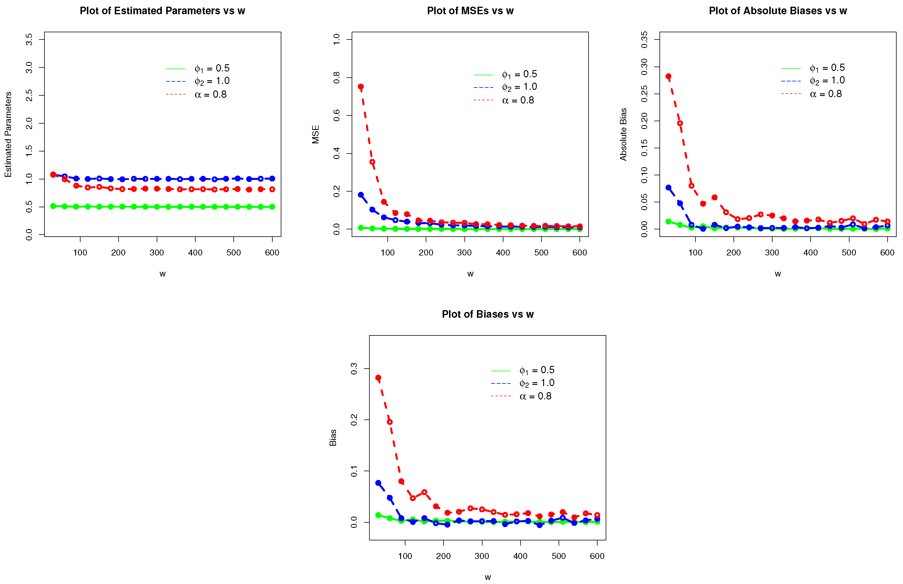
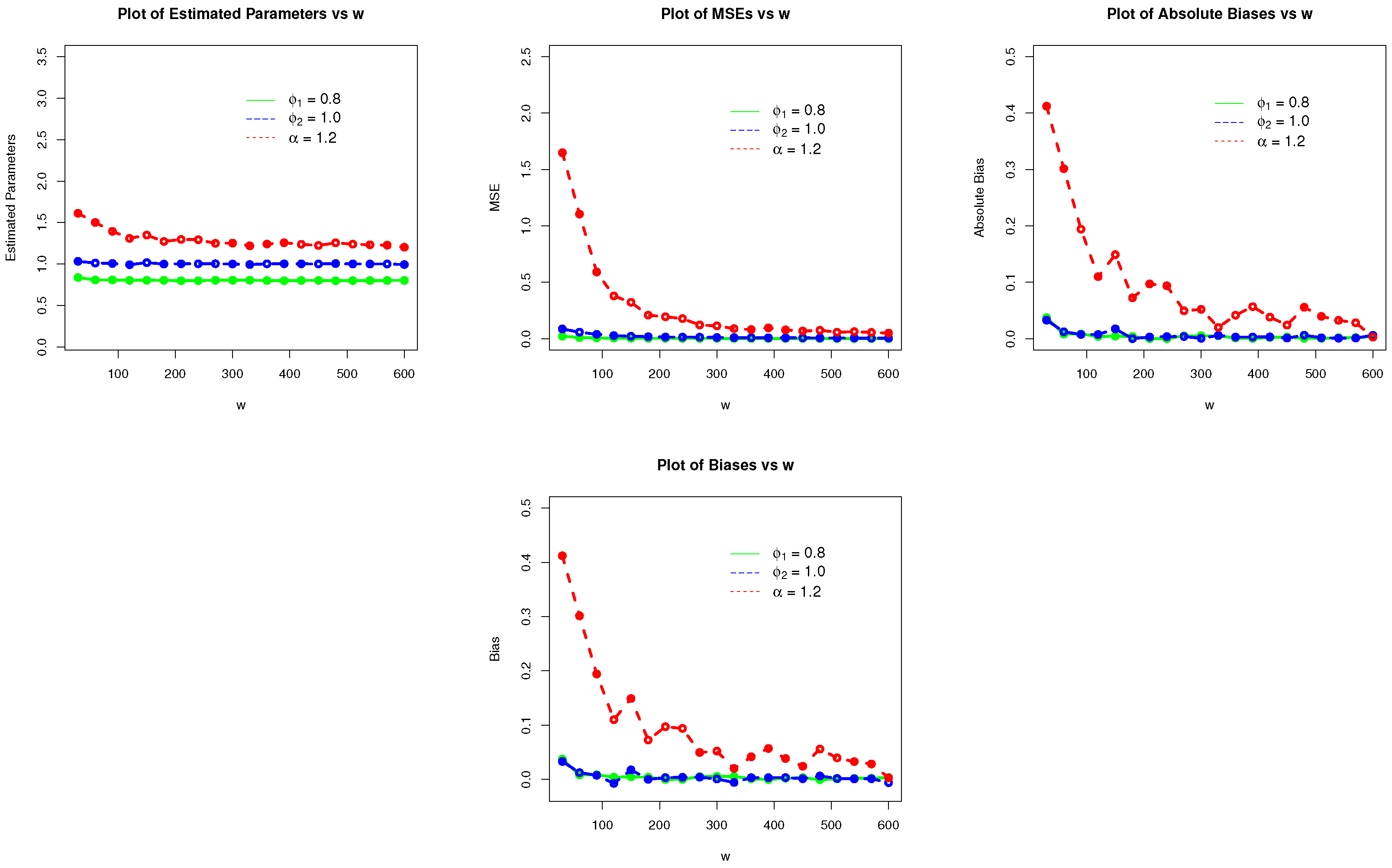
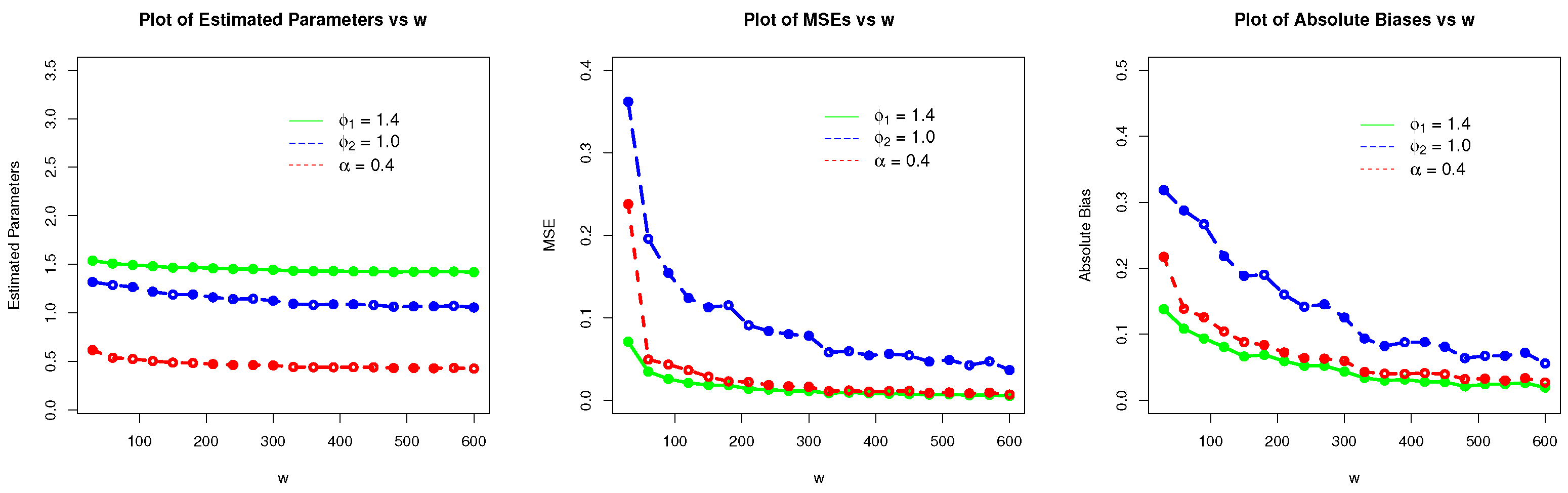
4. Estimation and Simulation

In this section, we use the ML (maximum likelihood) estimation approach to obtain the ML estimators α ^ , ϕ 1 ^ , and ϕ 2 ^ of the NME-Weibull parameters α , ϕ 1 , and ϕ 2 , respectively.
Suppose that X 1 , X 2 , , X w is a set of RS (random sample) of size, say w, taken from f x ; α , Λ . Then, linking to f x ; α , Λ , the LF (likelihood function), say Φ x ; α , Λ , is given by
Φ x ; α , Λ = i = 1 w f x i ; α , Λ ,
Using Equation (7) in Equation (15), we have
Φ x ; α , Λ = i = 1 w α 2 ϕ 1 ϕ 2 x i ϕ 1 1 e ϕ 2 x i ϕ 1 α + 1 e ϕ 2 x i ϕ 1 3 α + 2 1 e ϕ 2 x i ϕ 1 .
Corresponding to Equation (16), the log LF, say Ψ x ; α , Λ , is given by
Ψ x ; α , Λ = 2 w log α + w log ϕ 1 + w log ϕ 2 + ϕ 1 1 i = 1 w log x i ϕ 2 i = 1 w x i ϕ 1 + i = 1 w log α + 2 1 e ϕ 2 x i ϕ 1 3 i = 1 w log α + 1 e ϕ 2 x i ϕ 1 .
With respect to α , ϕ 1 , and ϕ 2 , the partial derivatives of Ψ x ; α , Λ are given by
α Ψ x ; α , Λ = 2 w α + i = 1 w 1 α + 2 1 e ϕ 2 x i ϕ 1 3 i = 1 w 1 α + 1 e ϕ 2 x i ϕ 1 ,
ϕ 1 Ψ x ; α , Λ = w ϕ 1 + i = 1 w log x i ϕ 2 i = 1 w log x i x i ϕ 1 i = 1 w log x i ϕ 2 x i ϕ 1 e ϕ 2 x i ϕ 1 α + 2 1 e ϕ 2 x i ϕ 1 , 3 i = 1 w log x i ϕ 2 x i ϕ 1 e ϕ 2 x i ϕ 1 α + 1 e ϕ 2 x i ϕ 1
and
ϕ 2 Ψ x ; α , Λ = w ϕ 2 i = 1 w x i ϕ 1 i = 1 w x i ϕ 1 e ϕ 2 x i ϕ 1 α + 2 1 e ϕ 2 x i ϕ 1 3 i = 1 w x i ϕ 1 e ϕ 2 x i ϕ 1 α + 1 e ϕ 2 x i ϕ 1 ,
respectively.
Setting α Ψ x ; α , Λ , ϕ 1 Ψ x ; α , Λ , and ϕ 2 Ψ x ; α , Λ to zero and solving them, we obtain the MLEs α ^ M L E , ϕ 1 ^ M L E , and ϕ 2 ^ M L E , respectively.
After obtaining the MLEs α ^ M L E , ϕ 1 ^ M L E , ϕ 2 ^ M L E of the NME-Weibull parameters, the next step is to investigate the performances of α ^ M L E , ϕ 1 ^ M L E , and ϕ 2 ^ M L E via a simulation study (SS).
The SS to evaluate α ^ M L E , ϕ 1 ^ M L E , and ϕ 2 ^ M L E is carried by three different combinations of α , ϕ 1 , and ϕ 2 . The combination values of α , ϕ 1 , and ϕ 2 are given by (i) α = 0.5 , ϕ 1 = 1.0 , ϕ 2 = 0.8 , (ii) α = 0.8 , ϕ 1 = 1.0 , ϕ 2 = 1.2 , and (iii) α = 1.4 , ϕ 1 = 1.0 , ϕ 2 = 0.4 . It is important to note that there are no hard and fast rules to select the initial values of the parameters to carry out the simulation studies. We can choose any values of the parameters within their range.
The SS is carried out by selecting an RS, say w = 30 , 60 , 90 , , 600 from f x ; α , Λ , using the inverse CDF method.
Finally, some statistical measures such as (i) MSEs, (ii) biases, and (iii) absolute biases are selected to see the performances of α ^ M L E , ϕ 1 ^ M L E , and ϕ 2 ^ M L E . The values of these statistical measures are, respectively, obtained as
M S E ( γ ^ ) = 1 600 i = 1 w γ ^ γ 2 ,
B i a s ( γ ^ ) = 1 600 i = 1 w γ ^ γ ,
and
| A b s o l u t e B i a s ( γ ^ ) | = | 1 600 i = 1 w γ ^ γ | ,
where γ ^ = α , ϕ 1 , ϕ 2 .
Corresponding to (a) α = 0.5 , ϕ 1 = 1.0 , ϕ 2 = 0.8 , (b) α = 0.8 , ϕ 1 = 1.0 , ϕ 2 = 1.2 , and (c) α = 1.4 , ϕ 1 = 1.0 , ϕ 2 = 0.4 , the results of the SS of the NME-Weibull model are presented in Table 1, Table 2 and Table 3. The results of the SS of the NME-Weibull model are also illustrated visually in Figure 3, Figure 4 and Figure 5. From the numerical illustration (i.e., Table 1, Table 2 and Table 3) and visual illustration (i.e., Figure 3, Figure 4 and Figure 5) of the simulation studies, we can easily observe that as the size of the samples increases, the
  • MLEs α ^ M L E , ϕ 1 ^ M L E , and ϕ 2 ^ M L E tend to stable.
  • MSEs of α ^ M L E , ϕ 1 ^ M L E , and ϕ 2 ^ M L E decrease.
  • Biases of α ^ M L E , ϕ 1 ^ M L E , and ϕ 2 ^ M L E tend to zero.

5. Practical Application

Here, we provide a practical application/illustration of the NME-Weibull distribution by analyzing the recovery time of the basketball players after an injury. Some basic measures (BMs) of the recovery time of the basketball players’ dataset are range = 15.47, variance = 15.93316, median = 8.710, minimum = 1.170, mean = 8.488, skewness = −0.00871759, 1 st quartile = 6.240, kurtosis = 2.230146, 3 rd quartile = 11.440, and maximum = 16.640. A visual display of the behavior of the recovery time of the basketball players’ dataset is provided in Figure 6.
The numerical results (fitting power) of the NME-Weibull distribution are compared with the
  • Weibull distribution with CDF, given by
    T x ; Λ = 1 e ϕ 2 x ϕ 1 , x 0 , ϕ 1 , ϕ 2 > 0 .
  • Exponentiated Weibull (E-Weibull) distribution with CDF, expressed by
    T x ; τ , Λ = 1 e ϕ 2 x ϕ 1 τ , x 0 , ϕ 1 , ϕ 2 , τ > 0 .
  • Marshall Olkin Weibull (MO-Weibull) distribution with CDF, given below:
    T x ; η , Λ = 1 e ϕ 2 x ϕ 1 1 1 η e ϕ 2 x ϕ 1 , x 0 , ϕ 1 , ϕ 2 , η > 0 .
  • Flexible Weibull (F-Weibull) distribution with CDF, provided below:
    T x ; Λ = 1 e e ϕ 1 x ϕ 2 x , x 0 , ϕ 1 , ϕ 2 > 0 .
We select four information criteria (IC) to see the best fitting power of the NME-Weibull and other competing distributions. The values of these IC are computed as
A I C = 2 w Ψ x ; α , Λ ,
B I C = w log n 2 Ψ x ; α , Λ ,
C A I C = w log n 2 Ψ x ; α , Λ ,
and
H Q I C = 2 w log log n 2 Ψ x ; α , Λ ,
respectively.
Using the recovery time of the basketball players, the values of the MLEs α ^ M L E , ϕ 1 ^ M L E , ϕ 2 ^ M L E , η ^ M L E , and τ ^ M L E are presented in Table 4, whereas the values of the IC of the fitted models are provided in Table 5. As a rule of thumb, a probability model with the lowest values of the IC quantities is called the best competing model. Based on the numerical illustration in Table 5, it is clear that the NME-Weibull distribution is the best-suited model for analyzing the considered recovery time of the basketball players’ dataset.
Furthermore, the fitting results of the fitted distributions are compared visually in Figure 7. For this purpose, the plots of the fitted PDF, fitted CDF, fitted SF, and QQ (quantile–quantile) function are considered. The plots in Figure 7 reveal the best fitting capability of the NME-Weibull distribution as it closely follows the plots of the fitted PDF, CDF, and SF.

6. Concluding Remarks

The prime goal of this research was to propose a novel probability model for analyzing datasets in the sports and healthcare sector. The new model was named NME-Weibull distribution. Several properties along with the HT characteristics were calculated. The MLEs of the NME-Weibull distribution were also obtained. To illustrate the NME-Weibull distribution, a practical application was presented. The dataset represented the recovery time after the injuries in different basketball matches. The comparison of the NME-Weibull distribution was made with four other competing probability models. Based on four IC quantities, it was observed that the NME-Weibull distribution was the best competing model for analyzing the recovery time after the injuries in different basketball matches.
Since the proposed model is continuous-type distribution, it can only be applied to continuous phenomena. In the future, we are motivated to introduce a discrete version of the NME-Weibull distribution for analyzing the discrete datasets. We are also committed to introducing the bivariate version of the NME-Weibull distribution for analyzing the bivariate datasets. Furthermore, a regression model based on the NME-Weibull distribution can also be considered in the future.

Author Contributions

Conceptualization, H.M.A., O.H.O. and Z.A; methodology, H.M.A., O.H.O., and Z.A.; software, H.M.A., Z.A., F.K. and A.A.-A.H.E.-B.; validation, H.M.A. and Z.A.; formal analysis, H.M.A., O.H.O., Z.A. and F.K.; investigation, O.H.O. and A.A.-A.H.E.-B.; data curation, Z.A. and F.K.; writing—original draft preparation, H.M.A., O.H.O., Z.A., F.K. and A.A.-A.H.E.-B.; writing—review and editing, H.M.A., O.H.O. and Z.A.; visualization, H.M.A., Z.A., F.K. and A.A.-A.H.E.-B. All authors have read and agreed to the published version of the manuscript.

Funding

The authors extend their appreciation to the Deputyship for Research & Innovation, Ministry of Education in Saudi Arabia for funding this research work through the project number RI-44-0440.

Data Availability Statement

The data is available from the corresponding author upon reasonable request.

Conflicts of Interest

The authors declare no conflict of interest.

References

  1. Ahmad, Z.; Hamedani, G.G.; Butt, N.S. Recent developments in distribution theory: A brief survey and some new generalized classes of distributions. Pak. J. Stat. Oper. Res. 2019, 15, 87–110. [Google Scholar] [CrossRef]
  2. Bannick, M.S.; McGaughey, M.; Flaxman, A.D. Ensemble modelling in descriptive epidemiology: Burden of disease estimation. Int. J. Epidemiol. 2020, 49, 2065–2073. [Google Scholar] [CrossRef]
  3. Deep, S.; Sarkar, A.; Ghawat, M.; Rajak, M.K. Estimation of the wind energy potential for coastal locations in India using the Weibull model. Renew. Energy 2020, 161, 319–339. [Google Scholar] [CrossRef]
  4. Mathlouthi, M.; Lebdi, F. Estimating extreme dry spell risk in Ichkeul Lake Basin (Northern Tunisia): A comparative analysis of annual maxima series with a Gumbel distribution. Proc. Int. Assoc. Hydrol. Sci. 2020, 383, 241–248. [Google Scholar] [CrossRef]
  5. Mori, H.; Chen, X.; Leung, Y.F.; Shimokawa, D.; Lo, M.K. Landslide hazard assessment by smoothed particle hydrodynamics with spatially variable soil properties and statistical rainfall distribution. Can. Geotech. J. 2020, 57, 1953–1969. [Google Scholar] [CrossRef]
  6. Alotaibi, R.; Okasha, H.; Rezk, H.; Almarashi, A.M.; Nassar, M. On a new flexible Lomax distribution: Statistical properties and estimation procedures with applications to engineering and medical data. AIMS Math. 2021, 6, 13976–13999. [Google Scholar] [CrossRef]
  7. Benatmane, C.; Zeghdoudi, H.; Shanker, R.; Lazri, N. Composite Rayleigh-Pareto distribution: Application to real fire insurance losses data set. J. Stat. Manag. Syst. 2021, 24, 545–557. [Google Scholar] [CrossRef]
  8. Shafqat, A.; Huang, Z.; Aslam, M. Design of X-bar control chart based on Inverse Rayleigh Distribution under repetitive group sampling. Ain Shams Eng. J. 2021, 12, 943–953. [Google Scholar] [CrossRef]
  9. Alevizakos, V.; Koukouvinos, C. Monitoring reliability for a gamma distribution with a double progressive mean control chart. Qual. Reliab. Eng. Int. 2021, 37, 199–218. [Google Scholar] [CrossRef]
  10. Lei, Z.; Shen, J.; Wang, J.; Qiu, Q.; Zhang, G.; Chi, S.S.; Wang, C. Composite polymer electrolytes with uniform distribution of ionic liquid-grafted ZIF-90 nanofillers for high-performance solid-state Li batteries. Chem. Eng. J. 2021, 412, 128733. [Google Scholar] [CrossRef]
  11. Kania, A.; Berent, K.; Mazur, T.; Sikora, M. 3D printed composites with uniform distribution of Fe3O4 nanoparticles and magnetic shape anisotropy. Addit. Manuf. 2021, 46, 102149. [Google Scholar] [CrossRef]
  12. Alfaer, N.M.; Gemeay, A.M.; Aljohani, H.M.; Afify, A.Z. The extended log-logistic distribution: Inference and actuarial applications. Mathematics 2021, 9, 1386. [Google Scholar] [CrossRef]
  13. Alshenawy, R. The Generalization Inverse Weibull Distribution Related to X-Gamma Generator Family: Simulation and Application for Breast Cancer. J. Funct. Spaces 2022, 2022, 4693490. [Google Scholar] [CrossRef]
  14. Almetwally, E.M. The odd Weibull inverse topp–leone distribution with applications to COVID-19 data. Ann. Data Sci. 2022, 9, 121–140. [Google Scholar] [CrossRef]
  15. Bo, W.; Ahmad, Z.; Alanzi, A.R.; Al-Omari, A.I.; Hafez, E.H.; Abdelwahab, S.F. The current COVID-19 pandemic in China: An overview and corona data analysis. Alex. Eng. J. 2022, 61, 1369–1381. [Google Scholar] [CrossRef]
  16. Rafique, M.; Ali, S.; Shah, I.; Ashraf, B. A comparison of different Bayesian models for leukemia data. Am. J. Math. Manag. Sci. 2022, 41, 244–258. [Google Scholar] [CrossRef]
  17. Shengjie, G.; Craig, A.; Mekiso, G.T. A New Alpha Power Weibull Model for Analyzing Time-to-Event Data: A Case Study from Football. Math. Probl. Eng. 2022, 2022, 7257264. [Google Scholar] [CrossRef]
  18. Penn, M.J.; Donnelly, C.A. Analysis of a double Poisson model for predicting football results in Euro 2020. PLoS ONE 2022, 17, e0268511. [Google Scholar] [CrossRef]
  19. Almalki, S.J.; Nadarajah, S. Modifications of the Weibull distribution: A review. Reliab. Eng. Syst. Saf. 2014, 124, 32–55. [Google Scholar] [CrossRef]
  20. Wilson, P.S.; Toumi, R. A fundamental probability distribution for heavy rainfall. Geophys. Res. Lett. 2005, 32, L14812. [Google Scholar] [CrossRef]
  21. Costa, U.M.S.; Freire, V.N.; Malacarne, L.C.; Mendes, R.S.; Picoli, S., Jr.; De Vasconcelos, E.A.; da Silva, E.F., Jr. An improved description of the dielectric breakdown in oxides based on a generalized Weibull distribution. Phys. A Stat. Mech. Appl. 2006, 361, 209–215. [Google Scholar] [CrossRef]
  22. Sartori, I.; de Assis, E.M.; da Silva, A.L.; de Melo, R.L.V.; Borges, E.P. Reliability modeling of a natural gas recovery plant using q-Weibull distribution. In Computer Aided Chemical Engineering; Elsevier: Amsterdam, The Netherlands, 2009; Volume 27, pp. 1797–1802. [Google Scholar]
  23. Zhang, F.; Ng, H.K.T.; Shi, Y. On alternative q-Weibull and q-extreme value distributions: Properties and applications. Phys. A Stat. Mech. Appl. 2018, 490, 1171–1190. [Google Scholar] [CrossRef]
  24. Hristopulos, D.T.; Baxevani, A. Kaniadakis Functions beyond Statistical Mechanics: Weakest-Link Scaling, Power-Law Tails, and Modified Lognormal Distribution. Entropy 2022, 24, 1362. [Google Scholar] [CrossRef]
  25. Carta, J.A.; Ramirez, P.; Velazquez, S. A review of wind speed probability distributions used in wind energy analysis: Case studies in the Canary Islands. Renew. Sustain. Energy Rev. 2009, 13, 933–955. [Google Scholar] [CrossRef]
  26. Papalexiou, S.M. Rainfall Generation Revisited: Introducing CoSMoS-2s and Advancing Copula-Based Intermittent Time Series Modeling. Water Resour. Res. 2022, 58, e2021WR031641. [Google Scholar] [CrossRef]
  27. Zhao, Y.; Ahmad, Z.; Alrumayh, A.; Yusuf, M.; Aldallal, R.; Elshenawy, A.; Riad, F.H. A novel logarithmic approach to generate new probability distributions for data modeling in the engineering sector. Alex. Eng. J. 2022, 62, 313–325. [Google Scholar] [CrossRef]
  28. El-Morshedy, M.; Ahmad, Z.; Almaspoor, Z.; Eliwa, M.S.; Iqbal, Z. A new statistical approach for modeling the bladder cancer and leukemia patients data sets: Case studies in the medical sector. Math. Biosci. Eng. 2022, 19, 10474–10492. [Google Scholar] [CrossRef]
  29. Ahmad, Z.; Almaspoor, Z.; Khan, F.; Alhazmi, S.E.; El-Morshedy, M.; Ababneh, O.Y.; Al-Omari, A.I. On fitting and forecasting the log-returns of cryptocurrency exchange rates using a new logistic model and machine learning algorithms. AIMS Math. 2022, 7, 18031–18049. [Google Scholar] [CrossRef]
  30. Ahmad, Z.; Mahmoudi, E.; Roozegar, R.; Alizadeh, M.; Afify, A.Z. A new exponential-X family: Modeling extreme value data in the finance sector. Math. Probl. Eng. 2021, 2021, 8759055. [Google Scholar] [CrossRef]
  31. Bhati, D.; Ravi, S. On generalized log-Moyal distribution: A new heavy tailed size distribution. Insur. Math. Econ. 2018, 79, 247–259. [Google Scholar] [CrossRef]
  32. Beirlant, J.; Matthys, G.; Dierckx, G. Heavy-tailed distributions and rating. ASTIN Bull. J. IAA 2001, 31, 37–58. [Google Scholar] [CrossRef]
  33. Seneta, E. Karamata’s characterization theorem, feller and regular variation in probability theory. Publ. L’Institut Mathématique 2002, 71, 79–89. [Google Scholar] [CrossRef]
Figure 1. Some possible shapes of f x ; α , Λ of the NME-Weibull model.
Axioms 12 00477 g001
Figure 2. Some possible shapes of h x ; α , Λ of the NME-Weibull model.
Axioms 12 00477 g002
Figure 3. Visual display of the numerical results of the SS of the NME-Weibull model for α = 0.5 , ϕ 1 = 1.0 , and ϕ 2 = 0.8 .
Axioms 12 00477 g003
Figure 4. Visual display of the numerical results of the SS of the NME-Weibull model for α = 0.8 , ϕ 1 = 1.0 , and ϕ 2 = 1.2 .
Axioms 12 00477 g004
Figure 5. Visual display of the numerical results of the SS of the NME-Weibull model for α = 1.4 , ϕ 1 = 1.0 , and ϕ 2 = 0.4 .
Axioms 12 00477 g005aAxioms 12 00477 g005b
Figure 6. A visual display of the behavior of the recovery time of the basketball players’ dataset.
Axioms 12 00477 g006
Figure 7. A visual display of the fitted results of the NME-Weibull and other competing distributions.
Axioms 12 00477 g007
Table 1. The numerical results of the SS of the NME-Weibull model for α = 0.5 , ϕ 1 = 1.0 , and ϕ 2 = 0.8 .
wParametersMLEsMSEsBiases
ϕ 1 0.51394480.00728900.01394476
30 ϕ 2 1.07683460.18123940.07683460
α 1.08235000.75237860.28234996
ϕ 1 0.50790460.00367780.00790461
60 ϕ 2 1.04767580.10271390.04767583
α 0.99577420.35492990.19577419
ϕ 1 0.50261370.00195580.00261367
90 ϕ 2 1.00795730.06239150.00795731
α 0.88007150.14397120.08007147
ϕ 1 0.50137300.00113320.00137297
150 ϕ 2 1.00795310.03949220.00795305
α 0.85871960.07925100.05871963
ϕ 1 0.50232440.00083970.00232438
240 ϕ 2 1.00350470.02371480.00350473
α 0.82041440.03627130.02041444
ϕ 1 0.50035120.00057810.00035115
330 ϕ 2 1.00231570.01643100.00231569
α 0.81992990.02639090.01992986
ϕ 1 0.50161300.00041970.00161304
420 ϕ 2 1.00155460.01346690.00155455
α 0.81555590.02083590.01555592
ϕ 1 0.50043100.00034170.00043099
480 ϕ 2 1.00292970.01118180.00292967
α 0.81518550.01718380.01518546
ϕ 1 0.50077760.00034140.00077761
510 ϕ 2 1.00876980.01238620.00876977
α 0.81992800.01774540.01992804
ϕ 1 0.50019250.00029440.00019245
570 ϕ 2 1.00366290.00968040.00366289
α 0.81733640.01484890.01733639
ϕ 1 0.50107610.00028910.00107609
600 ϕ 2 1.00668320.00991130.00668317
α 0.81412100.01473060.01412103
Table 2. The numerical results of the SS of the NME-Weibull model for α = 0.8 , ϕ 1 = 1.0 , and ϕ 2 = 1.2 .
wParametersMLEsMSEsBiases
ϕ 1 0.83735970.02284003.7359 × 10 2
30 ϕ 2 1.03296870.08641160.03296874
α 1.61223301.64929610.41223290
ϕ 1 0.80812820.01012498.1282 × 10 3
60 ϕ 2 1.01243010.05797910.01243010
α 1.50156001.10458640.30155973
ϕ 1 0.80850940.00673308.5094 × 10 3
90 ϕ 2 1.00751270.03905730.00751267
α 1.39428500.59150420.19428471
ϕ 1 0.80452680.00437084.5268 × 10 3
150 ϕ 2 1.01743120.02214280.01743116
α 1.34906000.32302410.14906040
ϕ 1 0.80004020.00257464.0247 × 10 5
240 ϕ 2 1.00374660.01448820.00374658
α 1.29385000.17806480.09384972
ϕ 1 0.80528710.00194285.2870 × 10 3
330 ϕ 2 0.99423570.0099813−0.00576426
α 1.22011700.08960110.02011655
ϕ 1 0.80199340.00142041.9934 × 10 3
420 ϕ 2 1.00324990.00783250.00324990
α 1.23829600.07815960.03829620
ϕ 1 0.79941540.0014117−5.8456 × 10 4
480 ϕ 2 1.00621470.00740680.00621474
α 1.25580400.07512550.05580425
ϕ 1 0.80064310.00129156.4306 × 10 4
510 ϕ 2 1.00168680.00616420.00168683
α 1.23960200.05712750.03960178
ϕ 1 0.80205530.00110902.0552 × 10 3
570 ϕ 2 1.00108320.00554880.00108320
α 1.22834700.05596100.02834659
ϕ 1 0.80336560.00108783.3655 × 10 3
600 ϕ 2 0.99388320.0058198−0.00611684
α 1.20284300.04991040.00284281
Table 3. The numerical results of the SS of the NME-Weibull model for α = 1.4 , ϕ 1 = 1.0 , and ϕ 2 = 0.4 .
wParametersMLEsMSEsBiases
ϕ 1 1.53813200.07092850.13813181
30 ϕ 2 1.31842800.36180160.31842754
α 0.61725100.23774040.21725102
ϕ 1 1.50846800.03474650.10846768
60 ϕ 2 1.28759900.19571310.28759929
α 0.53870650.04936680.13870647
ϕ 1 1.49359200.02587120.09359157
90 ϕ 2 1.26684500.15434030.26684505
α 0.52577740.04335620.12577736
ϕ 1 1.46642600.01849800.06642592
150 ϕ 2 1.18847700.11256130.18847743
α 0.48817620.02851090.08817621
ϕ 1 1.45223800.01297070.05223845
240 ϕ 2 1.14161200.08390580.14161192
α 0.46403790.01853090.06403786
ϕ 1 1.43378100.00879920.03378078
330 ϕ 2 1.09364300.05810370.09364311
α 0.44284180.01103100.04284176
ϕ 1 1.42800800.00800390.02800806
420 ϕ 2 1.08812800.05617040.08812753
α 0.44125270.01120330.04125268
ϕ 1 1.42102700.00689600.02102729
480 ϕ 2 1.06388000.04698170.06387966
α 0.43211810.00887330.03211808
ϕ 1 1.42419800.00723420.02419761
510 ϕ 2 1.06728800.04883790.06728819
α 0.43268150.00943590.03268150
ϕ 1 1.42624900.00646560.02624945
570 ϕ 2 1.07204400.04716510.07204448
α 0.43357960.00929250.03357964
ϕ 1 1.41932700.00526980.01932710
600 ϕ 2 1.05582200.03659560.05582239
α 0.42700030.00694400.02700025
Table 4. The values of α ^ M L E , ϕ 1 ^ M L E , ϕ 2 ^ M L E , η ^ M L E , and τ ^ M L E of the models.
Dist. α ^ ϕ 1 ^ ϕ 2 ^ η ^ τ ^
NME-Weibull12.367472.245150.00583--
Weibull-2.207680.00721--
Exponentiated Weibull-2.422470.00365-0.83154
Marshall Olkin Weibull-1.837850.024562.47454-
Flexible Weibull-0.1052918.14488--
Table 5. The values of the IC of the competitive models.
Dist.AICCAICBICHQIC
NME-Weibull431.3646431.6889438.4347434.1949
Weibull438.8245438.9845443.5379440.7114
E-Weibull439.5629439.8872446.6330442.3932
MO-Weibull438.8344439.1587445.9045441.6647
F-Weibull445.5514445.7114450.2648447.4382
Disclaimer/Publisher’s Note: The statements, opinions and data contained in all publications are solely those of the individual author(s) and contributor(s) and not of MDPI and/or the editor(s). MDPI and/or the editor(s) disclaim responsibility for any injury to people or property resulting from any ideas, methods, instructions or products referred to in the content.

