1. Introduction
In the statistical sciences, the process of hypothesis testing involves making an analyzed assumption about a population parameter for testing. To test the null hypothesis against an alternative hypothesis, analysts use a sample of the population. The null hypothesis usually states that two parameters are identical. For example, one can claim that the content means the payout is zero. The alternative hypothesis, such as “population means yield is not equal to zero” is essentially the opposite of the null hypothesis. Since they contradict each other, only one of them can be true.
Several classes of life models have been reported to reflect the different components of aging. In dependency, economics, queuing, epidemiology, scheduling, and other fields, the convex ascending order of random variables determined by the comparison of increasing and convex expectation functions has found wide use. A growing convex system has many applications in queuing theory, dependability, operations research, economics, and other fields. Stoyan [
1], for example, used this arrangement to determine the ideal sample size for an experimental design. By comparing queues and stochastic processes, Ross [
2] offered various applications of this ordering. Using a specific distribution order allows characterizing and creating new definitions of aging categories. The aging phenomenon refers to the fact that an older system rather than a younger one has a shorter residual life in some static sense. The lifespan distribution classes, such as
increasing failure rate (IFR),
increasing failure rate average (IFRA), and
new better than used (NBU), have thoroughly been researched usingreliability theory and its applications to derive practical constraints for the reliability of components or modules. The properties of maintaining life distribution classes under different reliability processes should also be studied for the same reason. These processes are generated by related systems, which may include identical or different components. Minimum and maximum component life, which are configured by the serial and parallel systems, respectively, are two important reliability measures.
Another well-liked action is warp, which is associated with cold standby systems. A lifetime distribution class is indicated as closed within a reliability process if the lifetime distributions of system components indicate that the lifetime distribution for the class as a whole also belongs to the class. It has long been found to be very useful in reliability theory for classifying life distributions according to aging characteristics. The most-well-known classes of life distributions that Barlow and Broshan [
3] examined are the characteristics of aging for our IFR, IFRA, and NBU. The
new better than used convex ordering (NBUC) and
new worse than used convex ordering (NWUC) aging qualities were both presented by Cao and Wang [
4] as extensions of NBU. Most of the traits connected to NBUC were investigated in Pellerey [
5]. For the
new better than used in the increasing convex average order (NBUCA) class based on the Laplace transform, see Al-Gashgari et al. [
6]. A
new better than used convex ordering moment generation function (NBUC
mgf) class was discussed by Abu-Youssef et al. [
7]. For the
exponential better than equilibrium life in convex (EBELC) class, see Mahmoud et al. [
8]. Many aging categories/classes for life distributions at specific ages have been explored from a variety of perspectives by statisticians and reliability analysts. More information can be found in Hollander et al. [
9]; Ebrahimi and Habbibullah [
10] considered the question of how to prove that the quality of an item, as measured by its residual life, has decreased after a certain period of time of time
This problem/issue may arise, for example, if one wishes to prove that the probability of failure has increased since the beginning of the process in order to justify the demand for certain maintenance activities at time
. Given that
is a given or definite period of interest, it is reasonable to assume that
is known. See Renea and Samanieg [
11] for NBU
, Ahmad [
12], Zehui and Xiaohu [
13] for IFRA
and NBU
, Mahmoud et al. [
14] for NBUE
, Mahmoud et al. [
15] for NBURFR
, Pandit and Anuradha [
16] for NBU
, Gadallah [
17] for NBU
, Abdul Alim [
18] for NBUFR
, Mahmoud et al. [
19] for NBUL
, Elbatal [
20] for NBUC
and NBU(2)
, and EL-Sagheer [
21] for NBRUL
. The main objective of the research is that in nonparametric testing of life distributions, we discovered a lack of test efficiency and a weak test power. To account for the effectiveness and strength of the test, we developed a brand-new reliability class test of the life distribution called a
new better than renewal used in the Laplace transform in increasing convex order at age (NBRULC
).
In actual life, there are instances when the system’s components gradually deteriorate up to time , the length of the warranty period most manufacturers provide, and are then renewed by the replacement of spare parts at time . In this situation, renewal aims to improve system usability, but is unable to restore the system to its previous state at age . For instance, the Aviation Administration decided that an airplane engine component needs to be replaced after many hours of flying. According to the airlines, this substitution is at best unneeded and might potentially be damaging to the aircraft. Airlines use operating data to determine whether an airplane engine is still as good as new after hours of renewal to back up their claim.
In the medical field, according to experts in the field of cancer, a person who has just received a diagnosis of a certain type of cancer has a significantly lower chance of surviving than someone alive for five years () since receiving the diagnosis. (In fact, such survivors are frequently labeled as “cured”.) There may be a desire to test the cancer professionals’ beliefs.
Furthermore, for instance, a component that a manufacturer claims exhibits “infant mortality” has a declining failure rate over the range . This notion is based on knowledge gained for related components. One wants to know if a used component of a certain age has a stochastically longer residual life than a fresh component. If so, he/she will test a certain portion of his/her output over the range and then sell the components that have survived to customers who require high-reliability components (such as a spacecraft assembly) at a premium price. To confirm or deny his/her preconceived notion, he/she wants to test this theory. The development of a new class of life distribution (NBRULC), a discussion of its characterization, and a comparison of the exponentiality and NBRULC class using the -statistic are the main points of this essay.
2. NBRULC Class: Interpretation and Characterization
2.1. Interpretation
A survival function
for a positive random variable
X is considered a
new better (worse) than renewal used in the Laplace transform order,
NBRUL (NWRUL), iff
where
x is the value of the random variable
X,
m represents the parameter of the exponential distribution, and
t is the time after a period of operation
(
) (see Mahmoud et al. [
22]). Depending on this concept, Etman et al. [
23] defined a new class, in the so-called a
new better (worse) than renewal used in Laplace transform in increasing convex order, say NBRULC (NWRULC), as follows
or
where
According to the definitions of Mahmoud et al. [
22] and Etman et al. [
23], a new class of life distributions known as NBRULC at age
, say (NBRULC
), is defined. A survival function
for a non-negative random variable
X is considered
new better (worse) than renewal used in the Laplace transform in increasing convex order at age ,
NBRULC
NWRULC
, iff
or
and this could be rewritten as
Remark 1. It is clear that NBRULNBRULCNBRULC.
2.2. Characterization
2.2.1. Convolution Property
The convolution property of reliability classes is a property that states that if a system has a certain reliability class, such as IFR or NBU, then any convolution of systems with the same reliability class will also have the same reliability class. A systems wrap is a system consisting of various components connected in series, such that the system fails when any of the components fail. The reliability class is a way to describe how the failure rate of a system has changed over time. One possible application of the convolution property of reliability classes is the reliability analysis of systems consisting of different components connected in series. For example, one can use the convolution property to determine whether a system consisting of regenerative convolutions has a certain reliability class, such as IFR or NBU. Regeneration is a process that defines the time between successive failures of a system that is either repaired or replaced after each failure. Some possible properties of reliability classes are: Save property This property states that if a system has a certain reliability class, such as IFR or NBU, any subsystem or component of the system will have the same reliability class. This characteristic indicates that adding more components to the system will not improve the reliability class; Close property This property states that if a system has a certain reliability class, such as IFR or NBU, then any function in the system that maintains its failure rate will also have the same reliability class. For example, if the system has an IFR class, then the reciprocal or logarithm will also have an IFR class; Duality property This property states that if a system has a certain reliability class, such as IFR or NBU, its dual system will have the opposite reliability class, such as DFR or NWU. A dual system is a system with the same failure rate as the original system but with an inverted time scale. For example, if a system has an IFR class, its dual system will have a DFR class. One possible way to use the properties of reliability classes to analyze systems is to perform a RAMS analysis. Using the properties of reliability classes, one can determine how the failure rate of a system changes over time and how it affects its availability and maintainability. For example, one can use the save property to compare reliability classes for different components or subsystems of a system. One can also use the closure property to apply different functions to the system and see how they affect the reliability class. One can also use the duality property to find system duality and compare reliability classes.
Theorem 1. The NBRULC class is preserved under convolution.
Proof. It is known that the convolution of two independent NBRULC
lifetime distributions,
and
, can be formulated as
Since
is NBRULC
, then
and by using
for
, we obtain
which completes the proof. □
2.2.2. Mixture Property
The mixing property of reliability classes is a property that states that if a system has a certain reliability class, such as IFR or NBU, any combination of systems with the same reliability class will also have the same reliability class. A mixture of systems is a system consisting of different components chosen randomly according to some probability distribution. The reliability class is a way to describe how the failure rate of a system has changed over time. One possible application of the mixture characteristic for reliability classes is the reliability analysis of systems consisting of different components with different lifetimes and different failure rates. For example, one can use the admixture property to determine whether a system consisting of a mixture of regeneration processes has a certain reliability class, such as IFR or NBU. Regeneration is a process that defines the time between successive failures of a system that is either repaired or replaced after each failure. One possible example of a system consisting of a mixture of regeneration processes is a system that detects and separates impulsive sources based on impulse spacing. The pulse spacing of each source is modeled as a regeneration process, which means that the time between successive pulses is a random variable that depends only on the previous impulse. The system receives a mixture of pulses from different sources and tries to determine which source each pulse belongs to. This is called deinterlacing of regeneration mixtures. The system filters out mixtures of regeneration processes using a method called maximum likelihood estimation (MLE). MLE is a technique that searches for the most likely values of statistical model parameters that fit the observed data. In this case, the system attempts to find the most likely values of the pulse spacing distributions for each source that fit the observed mixture of pulses. The system then assigns each pulse to the source that has the highest probability of generating it. Some of the potential advantages and disadvantages of MLE are: Advantages: It is easy to apply and can handle different types of statistical models. It has lower variance than other methods, which means it is less affected by sampling error. It is also unbiased with increasing sample size, which means that it converges to the true value of the coefficient. It is statistically well understood and has desirable properties such as consistency, efficiency, and approximate normality. Disadvantages: May be computationally intensive or intractable for some complex models. It may also be sensitive to outliers or model selection error. It does not account for prior information or parameter uncertainty. It may also result in biased estimates for small sample sizes.
Theorem 2. The NWRULC class is preserved under mixture.
Proof. It is obvious that
is the mixture of
, where each
is NWRULC
, where
then
since
is NWRULC
, then
Chebyshev’s inequality for similarity-ordered functions yields the following results
which complete the proof. □
Chebyshev’s inequality is a mathematical theorem that gives a limit on the probability that a random variable will deviate from its mean by more than a certain number of standard deviations. It can be used to estimate how likely it is that extreme values will be observed in a data set.
2.2.3. Homogeneous Poisson Shock Model
Homogeneous Poisson shock model is a type of stochastic model that describes system failure due to random shocks that occur according to the homogeneous Poisson process. Homogeneous Poisson process is a process that counts the number of events that occur in a given time period, where the events are independent and have a constant rate. The shock model assumes that each shock causes some damage to the system, and the system fails when the total damage exceeds a certain threshold. Poisson homogeneous shock models can be used to model various phenomena such as insurance claims, health impairment, or machine failure. For example, one can use a homogeneous Poisson shock model to estimate the probability of a car crashing due to random mechanical failures that occur at a constant rate over time. There are different types of trauma models depending on the nature and distribution of trauma and the damage it causes. For example, some common types of shock models are: Heterogeneous Poisson shock models, where shocks occur according to an in-homogeneous Poisson process with a variable rate over time; delta models-shocks, where shocks occur at fixed intervals and deal a fixed amount of damage; trigger shock models, where shocks occur in groups or combinations and deal a variable amount of damage; mixed shock models, where shocks are a mixture of different types of shock models. Note that these types of shock models differ from the types of circulatory shock that affect the human body, such as septic shock, cardiogenic shock, hypovolemic shock, or anaphylactic shock. Some of the potential advantages and disadvantages of inhomogeneous Poisson shock models are: Advantages: they can capture changes in the shock rate over time, which may better reflect the reality of some phenomena than a constant rate. They can also accommodate different types of shock rate functions, such as periodic, linear, exponential, or arbitrary functions. According to the disadvantages: they may be more complex and difficult to analyze than homogeneous Poisson shock models. It may also require more data and assumptions to estimate the parameters of the shock rate function. Some potential advantages and disadvantages of homogeneous Poisson shock models are: Advantages: They are simple and easy to analyze, as they only require one parameter to describe the shock rate. They can also model various phenomena such as insurance claims, health declines, or machine failures, by interpreting shocks as different types of events that affect the system. Disadvantages: It may not capture the fluctuation of shock rate over time, which may not reflect the reality of some phenomena that have variable or non-constant rates. They may also be too restrictive or unrealistic for some applications that require more flexibility or complexity in the shock model. Suppose the device is subjected to a series of shocks of force
k that occur randomly according to the Poisson process. Let us say the device has a probability
of surviving the first
s shocks, where
. Denote
. As a result, the device’s survival feature is provided by
where
k is the intensity constant in the shock model and
s represents the number of the shocks. This shock model has undergone research by Esary et al. [
24] for different aging properties, Klefsjo [
25] for HNBUE, and EL-Sagheer et al. [
26] for NBRUL.
Definition 1. A discrete distribution is said to have a discrete new better (worse) than renewal used in the Laplace transform in increasing convex order at age t (NBRULC) (NWRULC) if Theorem 3. If is discrete NBRULC, then given by (1) is NBRULC.
Proof. Upon using (1), we obtain
where
:
Let
:
since
F is NBRULC
:
Reversing the inequalities leads to the proof for the NWRULC class. □
3. Testing against NBRULC Alternatives
In this segment, we considered the possibility that is exponential in contrast to the corresponding hypothesis that it is not exponential, but NBRULC. Building our test statistic requires applying the following snippet/lemma.
Lemma 1. If the random variable X has a distribution function F that belongs to the NBRULC class, thenwhere Proof. Since
F is
, then
Integrating all sides with regard to
t over
results in
Similarly, if we set
then
Substituting (5) and (6) into (4), we obtain
and the proof is complete. The following entry point is suggested:
then
One can notice that the value of
under
equals
where
Consider that
could be expressed as follows:
An unbiased estimator of
is given by
The test statistic has asymptotic features that are reported in the following theorem: □
Theorem 4. (i) As is asymptotically normal with mean 0 and variance where(ii) Under the variance tends to Proof. Using standard
U-statistics theory (see Lee [
27]),
Using (8), we can find
and
as follows
and
Upon using (11–13), (9) is obtained. □
4. Pitman’s Asymptotic Efficiency of
Pitman’s asymptotic efficiency is a concept that measures the relative performance of two statistical tests in terms of their sample sizes. It is defined as the boundary of the proportion of minimum sample sizes required for each test to achieve a given level of significance and power, at which the alternative hypothesis approaches the null hypothesis. A higher Pitman’s efficiency means that the test requires fewer observations than another test to achieve the same accuracy. One possible application of the asymptotic Pitman efficiency is to compare different tests for different statistical problems and select the most efficient one. For example, one can use the asymptotic Pitman efficiency to compare different tests of equality of means, variances, or proportions between two populations. The asymptotic Pitman efficiency can also be used to compare different tests for the independence, correlation, or regression of two variables. Pitman efficiency can help the approach choose the best test for a given problem based on the minimum sample size required. Some potential limitations or assumptions of the asymptotic Pitman efficiency are: It is based on asymptotic results, which means that it may not be accurate for small or medium sample sizes. It also depends on the rate of convergence of test statistics for their finite distributions; sensitive to alternative hypothesis selection and level of significance. May not reflect performance of tests for alternatives or other levels; it does not take into account other factors that may influence test selection, such as robustness, simplicity, or interpretability. It also does not take into account the loss function or the cost of errors. Using the following probability models, the efficiency of the Pitman’s asymptotic efficiency (PAE) technique is assessed in this segment for the linear failure rate (LFR), Weibull, and Makeham distributions:
- (i)
The linear failure rate distribution (LFRD):
- (ii)
The Weibull distribution (WD):
- (iii)
The Makeham distribution (MD):
Be aware that
and
reduce to exponential distributions for
, while
reduces to an exponential distribution for
. The PAE is defined by
At
, this leads to
and
In
Table 1, different tests based on probability distributions are compared with the PAE test that is offered.
It is noted that the other tests that were studied in [
28,
29,
30] do not depend on
, while our proposed test depends on
and, therefore, gave better results compared to the results mentioned in
Table 1.
5. Monte Carlo Simulation
Monte Carlo simulation is a mathematical technique that uses random samples to estimate the possible outcomes of an uncertain event. It was invented by John von Neumann and Stanislaw Ulam during World War II. A Monte Carlo simulation works by predicting a set of outcomes based on an estimated range of values rather than fixed input values. It uses a probability distribution to generate random samples and then calculates the results for each sample. By repeating this process several times, it creates a distribution of possible outcomes that can be analyzed statistically. Some of the probability distributions that can be used in a Monte Carlo simulation are: the uniform distribution, all values have an equal probability of occurrence; Normal distribution, values are symmetrically distributed around a mean and a standard deviation; lognormal distribution, the values are positively skewed and have a logarithmic relationship with the mean and standard deviation; Exponential distribution, the values decrease exponentially and have a constant rate coefficient; binomial distribution, values are discrete and represent the number of successes in a fixed number of trials with a fixed probability of success; and Poisson distribution, the values are discrete and represent the number of events that occur in a fixed time interval or space with a fixed rate parameter. A Monte Carlo simulation can be used to estimate the probability of an event occurring by following these steps: select the event whose probability you want to estimate and select the random variables that affect it; determine the probability distribution of each random variable, and generate random samples from it; evaluate the event for each sample, and count how often it occurs; Divide the number of iterations by the total number of samples, and multiply by 100 to get the percentage; Repeat this process several times, and calculate the mean and standard deviation of the percentages. This will give you an estimate of the probability of the event and the uncertainty surrounding it.
5.1. Critical Points
A critical value in a statistic is a distribution point for a test statistic under the null hypothesis that identifies a set of values that invite a rejection of the null hypothesis. This group is called the critical region or rejection region. One-sided tests usually have one critical value and two-sided tests usually have two critical values. A critical value and a p-value are two different approaches to the same outcome: enabling you to support or reject the null hypothesis in a test. The difference is: a critical value is a fixed value that depends on the significance level and the type of test. You are comparing the test statistic to the critical value to make a decision. If the test statistic is more extreme than the critical value, you reject the null hypothesis. Whereas,
p-value is a calculated value based on the test statistic and distribution under the null hypothesis. The probability value is compared to the level of importance to make a decision. If the
p-value is less than or equal to the level of significance, you reject the null hypothesis. According to the statistical literature, there is no definitive answer to which approach is better: critical value or probability value. Both have advantages and disadvantages, depending on the situation and preference. Some factors to consider are: Critical values are easier to use when you have a table of values for common tests and significance levels.
p-values are easier to use when you have a calculator or software that can calculate them for any test and any level of significance; Critical values are more intuitive and visual, as they show the boundary between rejecting and not rejecting the null hypothesis.
p-values are more accurate and informative, because they show the exact probability of obtaining the test statistic or more extreme under the null hypothesis; Critical values are more conservative and less likely to make a type I error (rejecting the null hypothesis when it is true).
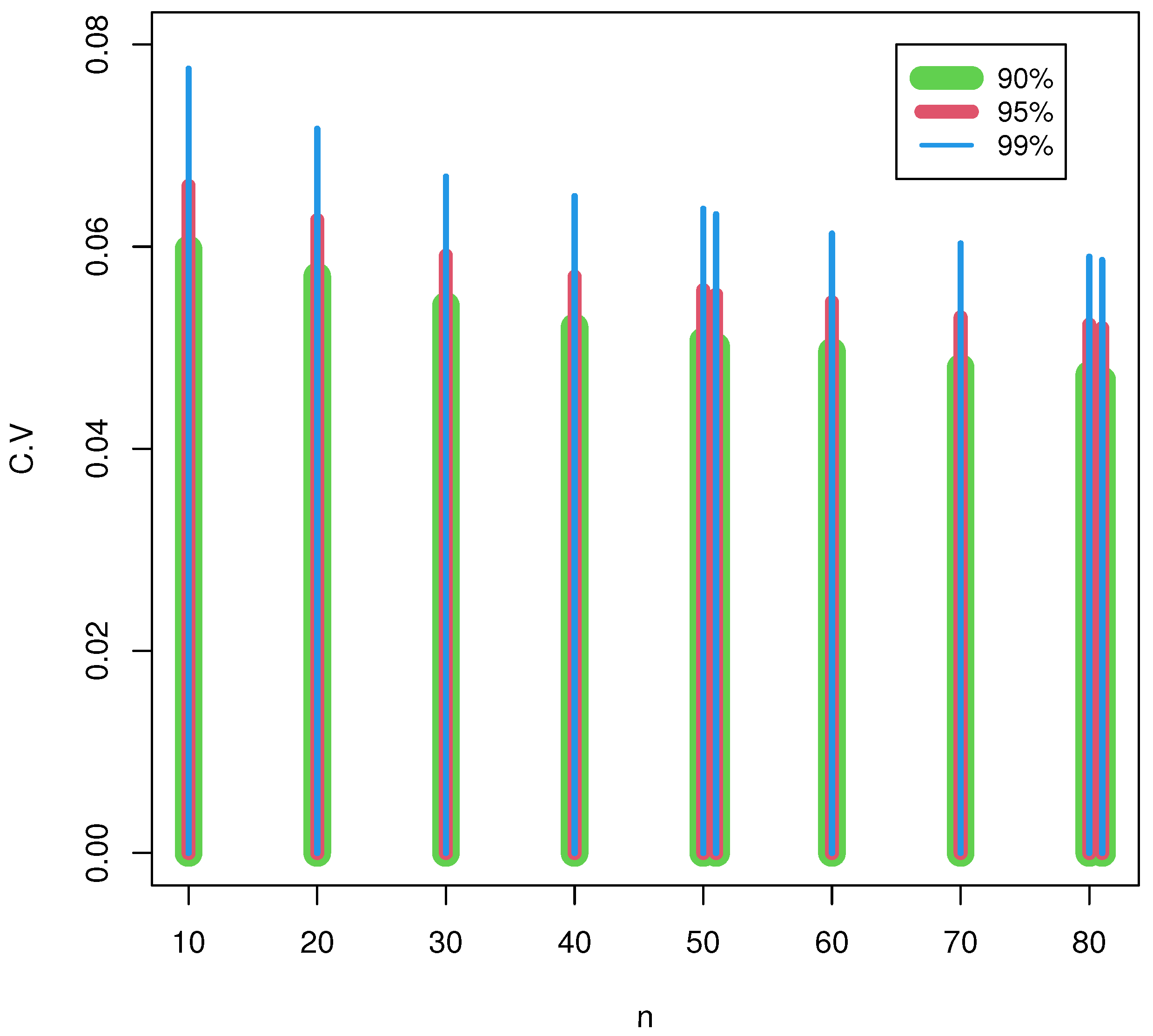
p-values are more flexible and less likely to make a type II error (not rejecting the null hypothesis when it is false). This segment mimics the null Monte Carlo distribution’s critical points utilizing 10,000 size-generated samples with
. The upper percentile of
for
, and
was determined. The critical values rose with the rising confidence levels and fell with the rising sample sizes, as noted in
Table 2 and
Figure 1, respectively.
5.2. Power Estimates of Test
Power estimates in Statistics are calculations that help you determine the minimum sample size for your study. Strength is the probability that the null hypothesis will be correctly rejected when it is false. It is based on four main components: effect size, difference size or relationship between variables of interest; significance level, probability of making a type I error (rejecting the null hypothesis when it is true); sample size and number of observations or study participants; and power, the probability of making a correct decision (rejecting the null hypothesis when it is false). If you know or have estimates for any three of these components, you can calculate the fourth using energy analysis. Energy analysis can help you design your study more efficiently and avoid wasting resources or missing out on important effects. A confidence interval is a range of values within which you would expect your estimate to fall if you retested, within a certain level of confidence. Statistical confidence is another way of describing probability. Power and confidence intervals are related in the following ways: Both power and confidence are probabilities dependent on the level of significance and sample size. A higher significance level or larger sample size will increase both power and confidence; Both strength and confidence are affected by impact size. A larger effect size will increase the strength and narrow the confidence interval; Both strength and confidence are inversely related. A higher power means a lower probability of making a type II error (not rejecting the null hypothesis when it is false), but also a higher probability of making a type I error (rejecting the null hypothesis when it is true). A higher confidence means a lower probability of making a type I error, but also a lower probability of making a type II error. Based on the 10,000 samples given in
Table 3, the power of the proposed test was estimated at the
confidence level,
. Assume appropriate parameter values of
for the LFRD, WD, and gamma distribution (GD), respectively, at
and 30.
Table 3 shows that the test we used
has good power for all other options.
5.3. Testing against NBRULC Class for Censored Data
A test statistic is suggested to compare
versus
using data that have been randomly right-censored. In a life-testing model or clinical study where patients may be lost (censored) before the completion of a study, such censored data are typically the only information available. Formally, this experimental scenario can be represented as follows. Assume that
n objects are tested, with
designating each object’s actual lifespan. Assuming a continuous life distribution
F, we let
be independently and identically distributed (i.i.d). Assume that, by a continuous life distribution
G,
are i.i.d. Furthermore, consider the
Xs and
Ys to be independent variables. We observed the pairs in the randomly right-censored model
where
and
Let
signify the ordered
Zs and
be
comparable to
Using the censored data (
),
Kaplan and Meier [
31] proposed the product limit estimator:
Now, for testing
against
using the data that were right-censored randomly, we recommend the following test statistic:
where
. It is possible to rewrite
for computing purposes as
where
and
To make the test invariant, let
The critical percentiles of the
test for sample sizes
are shown in
Table 4 and
Figure 2. Using the
Mathematica 12 program, the common exponential distribution was used to obtain the critical values at
and 10,000 replications for the null Monte Carlo distribution.
Following
Figure 2 and
Table 4, the critical values rose with the rises in the confidence level and fell with the rising sample sizes, respectively.
5.4. Power Estimates of Test
According to the three different Weibull, LFR, and gamma distributions based on 10,000 samples, the power of our test was evaluated at a significance level
with occasion parameter values of
at
and 30. For all other options,
Table 5 demonstrates that the power estimates of our test
were good.
6. Applications to Real Data: Censored and Uncensored Observations
Controlled (censored) data is only partially known data, which means that some information is missing or incomplete. Uncensored data is fully known data, which means that all information is available and complete. Controlled data can present challenges for statistical analysis, as it requires special methods and assumptions to deal with missing or incomplete information. Unsupervised (Uncensored) data is easier to analyze, because it does not have these issues.
6.1. Non-Censored Data
6.1.1. Dataset I: Aircraft’s Air Conditioning
The number of operational days between successive failures of an aircraft’s air conditioning system is a classic real dataset that Keating et al. [
32] examined. This information is documented.
| 3.750 | 0.417 | 2.500 | 7.750 | 2.542 | 2.042 | 0.583 |
| 1.000 | 2.333 | 0.833 | 3.292 | 3.500 | 1.833 | 2.458 |
| 1.208 | 4.917 | 1.042 | 6.500 | 12.917 | 3.167 | 1.083 |
| 1.833 | 0.958 | 2.583 | 5.417 | 8.667 | 2.917 | 4.208 |
| 8.667 | |
The shape of the data can be seen in
Figure 3, and it is noted that there is an extreme observation and the kernel density is right-skewed. The
was obtain, and this number is less than the value in
Table 2’s tabulated value. The significance level of
makes it clear. The NBRULC
attribute is not met by this type of data; hence, this is true.
6.1.2. Dataset II: Air Conditioning in a Boeing 720 Aircraft
The dataset below shows the 16 operational days between consecutive air conditioning system failures in a Boeing 720 aircraft (see Edgeman et al. [
33]).
| 4.25 | 8.708 | 0.583 | 2.375 | 2.25 | 1.333 | 2.792 | 2.458 |
| 5.583 | 6.333 | 1.125 | 0.583 | 9.583 | 2.75 | 2.542 | 1.417 |
Visualization plots of the data can be listed in
Figure 4, and it was observed that there is no extreme observation and that the intensity of the kernel tends to the right. When
was obtained, it is smaller than the relevant critical value in
Table 2, and the null hypotheses, which demonstrate that the dataset has an exponential feature, are accepted.
6.1.3. Dataset III: Leukemia
Consider the dataset below, which was compiled by Kotz and Johnson [
34] and shows the survival periods (in years) of 43 patients who had a specific type of leukemia after their diagnosis.
| 0.019 | 0.129 | 0.159 | 0.203 | 0.485 | 0.636 | 0.748 | 0.781 | 0.869 | 1.175 |
| 1.206 | 1.219 | 1.219 | 1.282 | 1.356 | 1.362 | 1.458 | 1.564 | 1.586 | 1.592 |
| 1.781 | 1.923 | 1.959 | 2.134 | 2.413 | 2.466 | 2.548 | 2.652 | 2.951 | 3.038 |
| 3.6 | 3.655 | 3.754 | 4.203 | 4.690 | 4.888 | 5.143 | 5.167 | 5.603 | 5.633 |
| 6.192 | 6.655 | 6.874 | | | | | | | |
The data representation plots are reported in
Figure 5, and it was found that there are no extreme observations and the nucleation intensity tends to the right. We obtained a value of
, which is below the crucial value in
Table 2. The null hypotheses were then accepted, proving that the dataset possesses exponential properties.
6.1.4. Dataset IV: COVID-19 in Italy
This data represents the COVID-19 mortality rate in Italy from 27 February to 27 April 2020 (see Almongy et al. [
35]). The data are
| | | | | | | | | |
| | | | | | | | | |
| | | | | | | | | |
| | | | | | | | | |
| | | | | | | | | |
| | | | | | | | | |
| | | | | | | | | |
Data representation plots are presented in
Figure 6, and it is clear that there are no extreme observations and the nucleation intensity tends to the right. When
was obtained, it is smaller than the relevant critical value in
Table 2, and the null hypotheses, which demonstrate that the dataset has an exponential feature, are accepted.
6.1.5. Dataset V: COVID-19 in the Netherlands
These data represent the COVID-19 mortality rate (see EL-Sagheer et al. [
36]). The data are
| | | | | | | | |
| | | | | | | | |
| | | | | | | | |
| | | | | | | | |
The data representation plots are sketched in
Figure 7, and it was found that there is an extreme observation and the intensity of nucleation tends to the right. At the significance level
is smaller than the corresponding critical value in
Table 2. This indicates that the type of data does not match the NBRULC
attribute.
6.2. Censored Data
6.2.1. Dataset VI: Myelogenous Blood Cancer
According to the International Bone Marrow Transplant Registry, 101 patients with advanced acute myelogenous blood cancer are represented by the following datasets (see Ghitany and Al-Awadhi [
37]). The data can be listed as:
| 0.030 | 0.493 | 0.855 | 1.184 | 1.283 | 1.480 | 1.776 | 2.138 | 2.500 |
| 2.763 | 2.993 | 3.224 | 3.421 | 4.178 | 4.441+ | 5.691 | 5.855+ | 6.941+ |
| 6.941 | 7.993+ | 8.882 | 8.882 | 9.145+ | 11.480 | 11.513 | 12.105+ | 12.796 |
| 12.993+ | 13.849+ | 16.612+ | 17.138+ | 20.066 | 20.329+ | 22.368+ | 26.776+ | 28.717+ |
| 28.717+ | 32.928+ | 33.783+ | 34.221+ | 34.770+ | 39.539+ | 41.118+ | 45.033+ | 46.053+ |
| 46.941+ | 48.289+ | 57.401+ | 58.322+ | 60.625+ | | | | |
Consider the entire set of survival data (both censored and uncensored). At a
confidence level,
is less than the critical value shown in
Table 4. Then, we agree with
, which asserts that the dataset has exponential features. The leukemia-free survival times for the 51 autologous transplant patients are (in months)
| 0.658 | 0.822 | 1.414 | 2.500 | 3.322 | 3.816 | 4.737 | 4.836+ | 4.934 |
| 5.033 | 5.757 | 5.855 | 5.987 | 6.151 | 6.217 | 6.447+ | 8.651 | 8.717 |
| 9.441+ | 10.329 | 11.480 | 12.007 | 12.007+ | 12.237 | 12.401+ | 13.059+ | 14.474+ |
| 15.000+ | 15.461 | 15.757 | 16.480 | 16.711 | 17.204+ | 17.237 | 17.303+ | 17.664+ |
| 18.092 | 18.092+ | 18.750+ | 20.625+ | 23.158 | 27.730+ | 31.184+ | 32.434+ | 35.921+ |
| 42.237+ | 44.638+ | 46.480+ | 47.467+ | 48.322+ | 56.086 | | | |
It was discovered that
, smaller than the critical value of
Table 4, was obtained. At the significance level
, it is obvious. This suggests that the data type does not align with the NBRULC
attribute.
6.2.2. Dataset VII: Melanoma
Consider the data in Susarla and Van Ryzin [
38]. These data show 46 melanoma patients’ survival rates. Of them, 35 correspond to entire lifetimes (non-censored data). The censored observations are listed in order:
| 13 | 14 | 19 | 19 | 20 | 21 | 23 | 23 | 25 | 26 |
| 26 | 27 | 27 | 31 | 32 | 34 | 34 | 37 | 38 | 38 |
| 40 | 46 | 50 | 53 | 54 | 57 | 58 | 59 | 60 | 65 |
| 65 | 66 | 70 | 85 | 90 | 98 | 102 | 103 | 110 | 118 |
| 124 | 130 | 136 | 138 | 141 | 234 | | | | |
The censored observations are ordered as follows:
| 16 | 21 | 44 | 50 | 55 | 67 | 73 | 76 | 80 | 81 |
| 86 | 93 | 100 | 108 | 114 | 120 | 124 | 125 | 129 | 130 |
| 132 | 134 | 140 | 147 | 148 | 151 | 152 | 152 | 158 | 181 |
| 190 | 193 | 194 | 213 | 215 | | | | | |
If we consider the entire set of survival data (both censored and uncensored), we found that the critical value in
Table 4 is more than our result, which is
. The data’s exponential qualities are thus clear to us.
7. Concluding Remarks
The emphasis on reliability has increased during the past few years among manufacturing companies, the government, and civilian groups. Attempts are being made by agencies to purchase systems that have higher reliability and require less frequent maintenance as a result of current worries regarding government spending. Buying products that are more dependable and require less upkeep is our top priority as consumers. Quality that holds up over time is reliable. Quality is related to craftsmanship and manufacture; thus, if something does not work or fails quickly after it is acquired, one would consider its quality to be bad. Poor reliability would, however, be present if, over time, product parts started to fail sooner than planned. Thus, the difference between quality and reliability is related to the passage of time and, more specifically, the product lifetime. The new life distribution class known as NBRULC is now a part of family of life distribution renewal classes. Convolution, mixture, and homogeneous shock models, among other reliability approaches, have all been used to create studies of closure qualities. After comparing the offered class test to some rival tests using the Weibull, LFR, gamma, and Makeham models, it was found that the suggested class performed well. A Monte Carlo simulation was run to evaluate the performance of NBRULC. It was discovered that, as the confidence levels climb and the sample sizes rise, the critical values also tend to rise. Furthermore, the power estimates of the suggested test were accurate based on the simulation results. To demonstrate the viability of the suggested NBRULC class, certain applications in the engineering and medical (censored and uncensored scenarios) domains were examined and addressed. Through the results, we concluded the following:
Author Contributions
Conceptualization, H.A. and M.S.E.; Methodology, M.E.-M., W.B.H.E. and R.M.E.-S.; Software, M.S.E., L.A.A.-E. and R.M.E.-S.; Validation, W.B.H.E., L.A.A.-E. and M.E.-M.; Formal analysis, H.A., R.M.E.-S. and M.E.-M.; Resources, M.E.-M. and L.A.A.-E.; Data curation, M.S.E. and R.M.E.-S.; Writing—original draft, R.M.E.-S. and W.B.H.E.; Writing—review & editing, M.S.E., W.B.H.E. and R.M.E.-S.; Supervision, H.A., M.E.-M. and W.B.H.E. All authors have read and agreed to the published version of the manuscript.
Funding
Princess Nourah bint Abdulrahman University Researchers Supporting Project and Prince Sattam bin Abdulaziz Universities under project numbers (PNURSP2023R443) and (PSAU/2023/R/1444), respectively.
Data Availability Statement
Data is reported within the article.
Acknowledgments
Princess Nourah bint Abdulrahman University Researchers Supporting Project number (PNURSP2023R443), Princess Nourah bint Abdulrahman University, Riyadh, Saudi Arabia. This study is supported via funding from Prince Sattam bin Abdulaziz University, project number (PSAU/2023/R/1444).
Conflicts of Interest
The authors declare no conflict of interest.
References
- Stoyan, D. Comparison Methods for Queues and Other Stochastic Models; Wiley: New York, NY, USA, 1983. [Google Scholar]
- Ross, S.M. Stochastic Processes; Wiley: New York, NY, USA, 1983. [Google Scholar]
- Barlow, R.E.; Proschan, F. Statistical Theory of Reliability and Life Testing; To Begin With: Silver Spring, MD, USA, 1981. [Google Scholar]
- Cao, J.; Wang, Y. The NBUC and NWUC classes of life distributions. J. Appl. Probab. 1991, 28, 473–479. [Google Scholar] [CrossRef]
- Pellerey, F. Shock models with underlying counting process. J. Appl. Probab. 1994, 31, 156–166. [Google Scholar] [CrossRef]
- Al-Gashgari, F.H.; Shawky, A.I.; Mahmoud, M.A.W. A nonparametric test for testing exponentiality against NBUCA class of life distributions based on Laplace transform. Qual. Reliab. Int. 2016, 32, 29–36. [Google Scholar] [CrossRef]
- Abu-Youssef, S.E.; Hassan, E.M.A.; Gerges, S.T. A new nonparametric class of life distributions based on ordering moment generating approach. J. Stat. Appl. Probability Lett. 2020, 7, 151–162. [Google Scholar]
- Mahmoud, M.A.W.; Diab, L.S.; Radi, D.M. Testing exponentiality against exponential better than equilibrium life in convex based on Laplace transformation. Int. J. Comput. Appl. 2018, 182, 6–10. [Google Scholar]
- Hollander, R.M.; Park, D.H.; Proschan, F. A class of life distributions for aging. J. Am. Stat. 1986, 81, 91–95. [Google Scholar] [CrossRef]
- Ebrahimi, N.; Habbibullah, M. Testing whether the survival distribution is new better than used of specified age. Biometrika 1990, 77, 212–215. [Google Scholar] [CrossRef]
- Renea, D.M.; Samanieg, F.J. Estimating the survival curve when new is better than used of a specified age. J. Am. Stat. Assoc. 1990, 85, 123–131. [Google Scholar] [CrossRef]
- Ahmad, I.A. Testing whether a survival distribution is new better than used of an unknown specified age. Biometrka 1998, 85, 451–456. [Google Scholar] [CrossRef]
- Zehui, L.; Xiaohu, L. IFRA*t0 and NBU*t0 classes of life distributions. J. Stat. Plan. Inference 1998, 70, 191–200. [Google Scholar] [CrossRef]
- Mahmoud, M.A.W.; Moshref, M.E.; Gadallah, A.M.; Shawky, A.I. New classes at specific age: Properties and testing hypotheses. J. Stat. Theory Appl. 2013, 12, 106–119. [Google Scholar] [CrossRef]
- Mahmoud, M.A.W.; Abdul Alim, N.A.; Diab, L.S. On the new better than used renewal failure rate at specified time. Econ. Qual. Control. 2009, 24, 87–99. [Google Scholar] [CrossRef]
- Pandit, P.V.; Anuradha, M.P. On testing exponentiality against new better than used of specified age. Stat. Methodol. 2007, 4, 13–21. [Google Scholar] [CrossRef]
- Gadallah, A.M. On NBUmgf-t0 class at specific age. Int. J. Reliab. Appl. 2016, 17, 107–119. [Google Scholar]
- Abdul Alim, N.A. Testing hypothesis for new class of life distribution NBUFR-t0. Int. J. Comput. 2013, 80, 25–29. [Google Scholar]
- Mahmoud, M.A.W.; Moshref, M.E.; Gadallah, A.M. On NBUL class at specific age. Int. J. Reliab. Appl. 2014, 15, 11–22. [Google Scholar]
- Elbatal, I. Some aging classes of life distributions at specific age. Int. Math. Forum 2007, 2, 1445–1456. [Google Scholar] [CrossRef]
- EL-Sagheer, R.M.; Mahmoud, M.A.W.; Etman, W.B.H. Characterizations and Testing Hypotheses for NBRUL-t∘ Class of Life Distributions. J. Stat. Theory Pract. 2022, 16, 31. [Google Scholar] [CrossRef]
- Mahmoud, M.A.W.; EL-Sagheer, R.M.; Etman, W.B.H. Testing exponentiality against new better than renewal used in Laplace transform order. J. Stat. Appl. Probab. 2016, 5, 279–285. [Google Scholar] [CrossRef]
- Etman, W.B.H.; EL-Sagheer, R.M.; Abu-Youssef, S.E.; Sadek, A. On some characterizations to NBRULC class with hypotheses testing application. Appl. Math. Inf. Sci. 2022, 16, 139–148. [Google Scholar]
- Esary, J.D.; Marshal, A.W.; Proschan, F. Shock models and wear processes. Ann. Probab. 1973, 1, 627–649. [Google Scholar] [CrossRef]
- Klefsjo, B. HNBUE survival under some shock models. Scand. J. Stat. 1981, 8, 39–47. [Google Scholar]
- EL-Sagheer, R.M.; Abu-Youssef, S.E.; Sadek, A.; Omar, K.M.; Etman, W.B.H. Characterizations and testing NBRUL class of life distributions based on Laplace transform technique. J. Stat. Appl. Probab. 2022, 11, 75–88. [Google Scholar]
- Lee, A.J. U-Statistics; Marcel Dekker: New York, NY, USA, 1989. [Google Scholar]
- Abdel Aziz, A.A. On testing exponentiality against RNBRUE alternatives. Appl. Math. Sci. 2007, 35, 1725–1736. [Google Scholar]
- Kango, A.I. Testing for new is better than used. Commun. Stat.-Theory Methods 1993, 12, 311–321. [Google Scholar]
- El-Morshedy, M.; Al-Bossly, A.; EL-Sagheer, R.M.; Almohaimeed, B.; Etman, W.B.H.; Eliwa, M.S. A Moment Inequality for the NBRULC Class: Statistical Properties with Applications to Model Asymmetric Data. Symmetry 2022, 14, 2353. [Google Scholar] [CrossRef]
- Kaplan, E.L.; Meier, P. Nonparametric estimation from incomplete observation. J. Am. Stat. 1958, 53, 457–481. [Google Scholar] [CrossRef]
- Keating, J.P.; Glaser, R.E.; Ketchum, N.S. Testing hypotheses about the shape of a gamma distribution. Technometrics 1990, 32, 67–82. [Google Scholar] [CrossRef]
- Edgeman, R.L.; Scott, R.C.; Pavur, R.J. A modified Kolmogorov-Smirnov test for the inverse Gaussian density with unknown parameters. Commun. Stat.-Simul. Comput. 1988, 17, 1203–1212. [Google Scholar] [CrossRef]
- Kotz, S.; Johnson, N.L. Encyclopedia of Statistical Sciences; Wiley: New York, NY, USA, 1983. [Google Scholar]
- Almongy, H.M.; Almetwally, E.M.; Aljohani, H.M.; Alghamdi, A.S.; Hafez, E.H. A new extended rayleigh distribution with applications of COVID-19 data. Results Phys. 2021, 23, 104012. [Google Scholar] [CrossRef]
- EL-Sagheer, R.M.; Eliwa, M.S.; Alqahtani, K.M.; EL-Morshedy, M. Asymmetric randomly censored mortality distribution: Bayesian framework and parametric bootstrap with application to COVID-19 data. J. Math. 2022, 2022, 8300753. [Google Scholar] [CrossRef]
- Ghitany, M.E.; Al-Awadhi, S. Maximum likelihood estimation of Burr XII distribution parameters under random censoring. J. Appl. Stat. 2002, 29, 955–965. [Google Scholar] [CrossRef]
- Susarla, V.; Vanryzin, J. Empirical Bayes estimations of a survival function right censored observation. Ann. Stat. 1978, 6, 710–755. [Google Scholar] [CrossRef]
| Disclaimer/Publisher’s Note: The statements, opinions and data contained in all publications are solely those of the individual author(s) and contributor(s) and not of MDPI and/or the editor(s). MDPI and/or the editor(s) disclaim responsibility for any injury to people or property resulting from any ideas, methods, instructions or products referred to in the content. |
© 2023 by the authors. Licensee MDPI, Basel, Switzerland. This article is an open access article distributed under the terms and conditions of the Creative Commons Attribution (CC BY) license (https://creativecommons.org/licenses/by/4.0/).


 ,
, 


