
First Entire Zagreb Index of Fuzzy Graph and Its Application


Department of Applied Mathematics with Oceanology and Computer Programming, Vidyasagar University, Midnapore 721 102, India
*
Author to whom correspondence should be addressed.
Axioms 2023, 12(5), 415; https://doi.org/10.3390/axioms12050415
Submission received: 24 March 2023
/
Revised: 18 April 2023
/
Accepted: 19 April 2023
/
Published: 24 April 2023
(This article belongs to the Special Issue Non-classical Logics and Related Algebra Systems)
Abstract
:The first entire Zagreb index (FEZI) is a graph parameter that has proven to be essential in various real-life scenarios, such as networking businesses and traffic management on roads. In this research paper, the FEZI was explored for a variety of fuzzy graphs, including star, firefly graph, cycle, path, fuzzy subgraph, vertex elimination, and edge elimination. This study presented several results, including determining the relationship between two isomorphic fuzzy graphs and between a path and cycle (connecting both end vertices of the path). This research also deals with the analysis of -cut fuzzy graphs and establishes bounds for some fuzzy graphs. To apply these findings to modern life problems, the research team utilized the results to identify areas that require more development in internet systems. These results have practical implications for enhancing the efficiency and effectiveness of internet systems. The conclusion drawn from this research can be used to inform future research and aid in the development of more efficient and effective systems in various fields.
Keywords:
first entire Zagreb index; second entire Zagreb index; first entire Zagreb index of a vertex; isomorphic graph; internet systemMSC:
05C09; 05C721. Introduction
1.1. Research Background
In the modern day, fuzzy graph (FG) theory is one of the most applicable to regular life. So there are many researchers who are implementing FG theory, especially topological indices of fuzzy graphs. Rosenfeld [1], inspired by Zadeh’s [2] classical set (fuzzy set) in 1975, introduced the fuzziness for a graph, then, it is called a fuzzy graph. Additionally, this time he introduced several connective parameters of an FG and some applications of these parameters by Yeh et al. [3]. In [4,5], Sunitha et al. studied fuzzy block, fuzzy bridge, FSG, CFG, PFSG, fuzzy tree, fuzzy forest, fuzzy cut vertex, etc. The degree of a vertex in an FG is also discussed In [6]. The degree of an edge () is also discussed in [7]. Further information on the FG hypothesis is provided in [8,9,10,11]. Bipolar and m-polar fuzzy graphs are discussed in [12,13]. The first Zagreb index is discussed in [14] and was inspired by the paper [15]. In a molecular graph of a chemical compound, we can calculate molecular descriptors by finding topological indices of this graph. A graph’s topology is described by these topological indices, which are numerical numbers. The Zagreb index, established in 1972 by Gutman and Trinajstic [16], is a degree-based topological index. The -electron energy of a conjugate system is determined using topological indices. In a crisp graph, many indices are defined but several issues in real life cannot be handled by these indices. So we can generalize these indices in fuzzy graphs. In this piece, we have introduced the FEZI in fuzzy graphs which is a major generalization of FEZI for crisp graphs. These indices are investigated from both a theoretical and an application point of view.
1.2. Research Question
These questions are covered in this paper:
- What is the FEZI upper bound for fuzzy graphs?
- What are the precise values or boundaries of FEZI for the firefly graph, star, path, cycle, etc.?
- What is the relation between the value of FEZI of a graph and its sub graph?
- What is the relation between the value of FEZI for two isomorphic graph?
- What is the relation for several graphs between the first Zagreb index and FEZI ?
- What are the applications of this index?
1.3. Objective of the Work
Various types of topological indices of a graph can be used for a variety of purposes and yield a wide range of outcomes for crisp graphs. However, in numerous applications, a crisp graph is not enough to solve it. We need to define a fuzzy graph to answer this question. In this paper, FEZI is defined and some results relating to sub graphs, paths, stars, firefly graphs, cycles, isomorphic graphs, etc. are given. At the end of this paper, we applied the first entire Zagreb index in internet network systems.
1.4. Structure of the Study
The structure of the article is as follows: in Section 2, some definitions are provided which are necessary for this study. In Section 3, we studied the FEZI of a fuzzy graph and provided some results on sub graphs, paths, stars, firefly graphs, cycles, etc. Also some relation between fuzzy graphs are provided. In Section 4, an application of the first entire Zagreb index in development in internet networking system is discussed.
2. Preliminaries
Here, we provide some fundamental definitions and theorems which are crucial to developing the later sections.
Let U be a universal set. An FS A on U is a mapping . Here, is the membership function of the FS A. A FS generally indicated by .
Assume that is a known finite set. Then the fuzzy graph (FG) is a triplet, , where with and satisfying . The set U is the set of vertices and is the set of edges of the FG. represents the membership value (MV) of the vertex and represents the MV of the edge (or ).
Let be an FG. Then, is called the PFSG of the FG G if for all . If and for all then H is called FSG of the graph of the FG G.
For , we denote as an FSG of the FG with and for , represents the FSG of the FG G with .
Let all be vertices of an FG G. Then, the collection of vertices is a path in G if (for all i). The path’s length is n in this case. If for the path then it is called a cycle.
Let be distinct vertices of a fuzzy graph G. Then, is called a star if for and for all vertex except there is no edge between every two vertices, where is the center of the star.
In a graph G if for all vertices and , then it is called a complete graph. In a fuzzy graph if for every two vertex x and y satisfy the condition then the graph is called a CFG.
Two FG and are called isomorphic to each other if there exists a bijective mapping for any , and .
Let be a crisp graph. Then, the first and second ZI are defined by and [17].
The total degree of an FG with respect to vertices is indicated by and is defined by [7]. Additionally, the total degree of an FG with respect to edge is indicated by and is defined by .
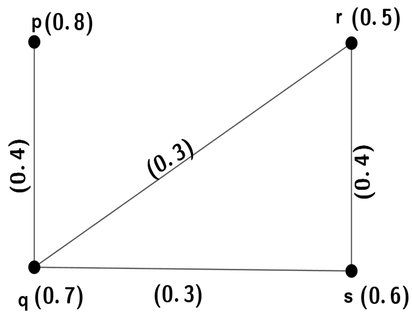
Example 1.
Let G be an FG with vertex set such that , as shown in Figure 1. Then, and and .
3. First Entire Zagreb Index of Fuzzy Graphs
First entire Zagreb index (FEZI) have an important role for finding strength of vertices. The strength of vertices is important in fuzzy graph theory. Thus, in this section the FEZI of a fuzzy graph is initiated. Various properties and an application of FEZI for fuzzy graphs is given.
Definition 1.
Let G be an FG. Then, the FEZI of G is indicated by and is defined by: .
Definition 2.
Let be an FG. Then, the second entire Zagreb index of G is indicated by and is defined by , where ω is the MV of a vertex and ϱ is the MV of an edge.
Figure 2.
A fuzzy graph G with = 1.0448.

Theorem 1.
Let the FG G have n vertices and m edges, then , where and represent the total degree with respect to vertex and total degree with respect to edge.
Proof.
Now, the FEZI of G is given by
.
Since , we have
.
Since and , therefore . □
Definition 3.
Let be an FG. Then FEZI at a vertex of G is indicated by and is defined by where .
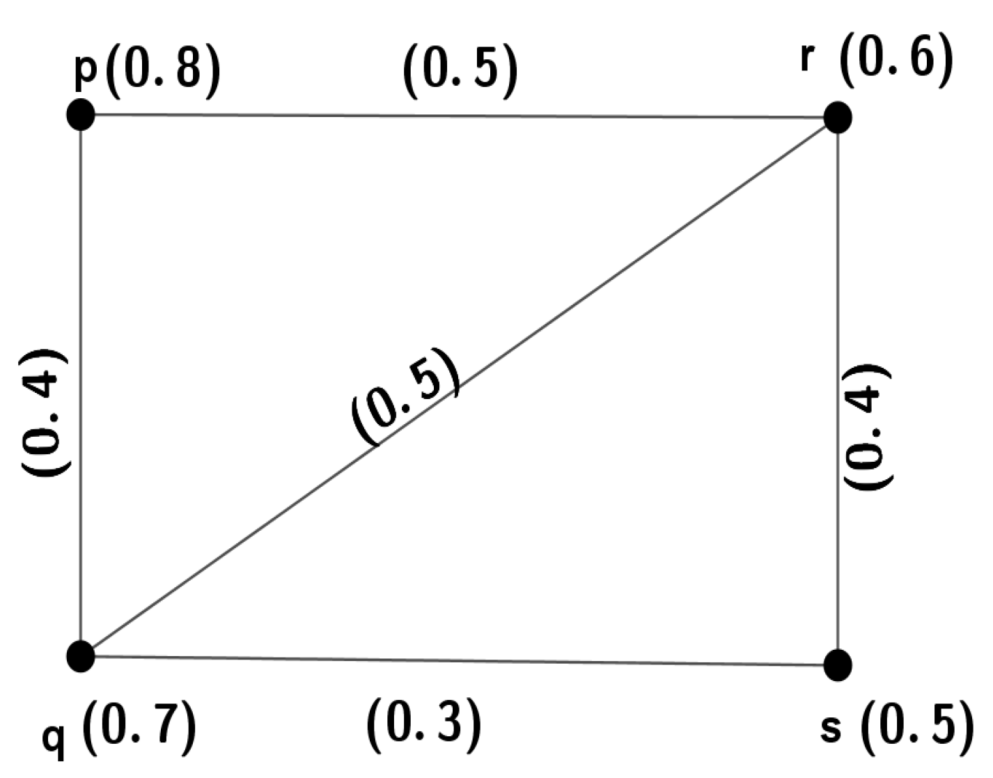
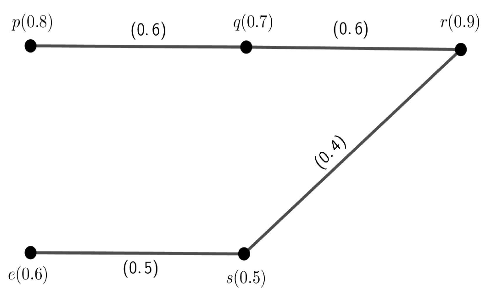
Example 4.
Let G be an FG with vertex set such that and shown in Figure 3. Then, .
Now,
So .
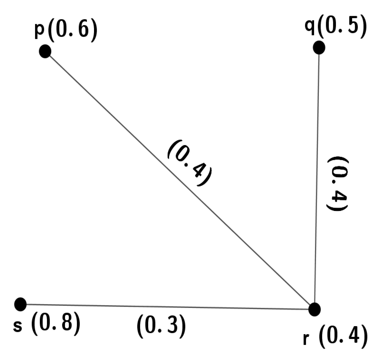
Now the vertex p is removed from the graph G, then the graph of is shown in Figure 4. From the figure, .
Now,
. Therefore, .
Then, the FEZI at p is .
Theorem 2.
Suppose that H is an FG that is created by removing an edge from G. Then, .
Proof.
Since is an FG and is a graph that is created by removing an edge from G so the MV of a vertex is the same in both graphs and the MV of edges are the same if it contains both E and .
Then, the relation between the membership values of G and H is for all vertices x and for all edges.
This shows that for all vertices x. Additionally, for all edge e, where d and represent the degree of G and H.
Now,
.
Hence, . □
Theorem 3.
If H is an FG that is obtained from G by deleting a vertex from G. Then, .
Proof.
Since is an FG and is a graph that is created by removing a vertex from G.
So, if otherwise . Additionally, if otherwise . Then the relation between the membership values of and is for all vertices x and for all edges e. This shows that for all vertices x. Additionally, for all edges e. Here, d and represent the degrees of G and H.
Now,
. So, . □
Example 5.
Let G be an FG with vertex set such that shown in Figure 3. Then and .
Now, .
.
The graph of H where the vertex p is deleted from G shown in Figure 4. From the figure, .
Now,
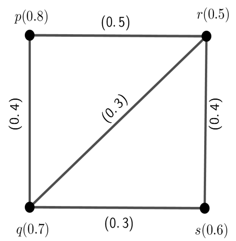
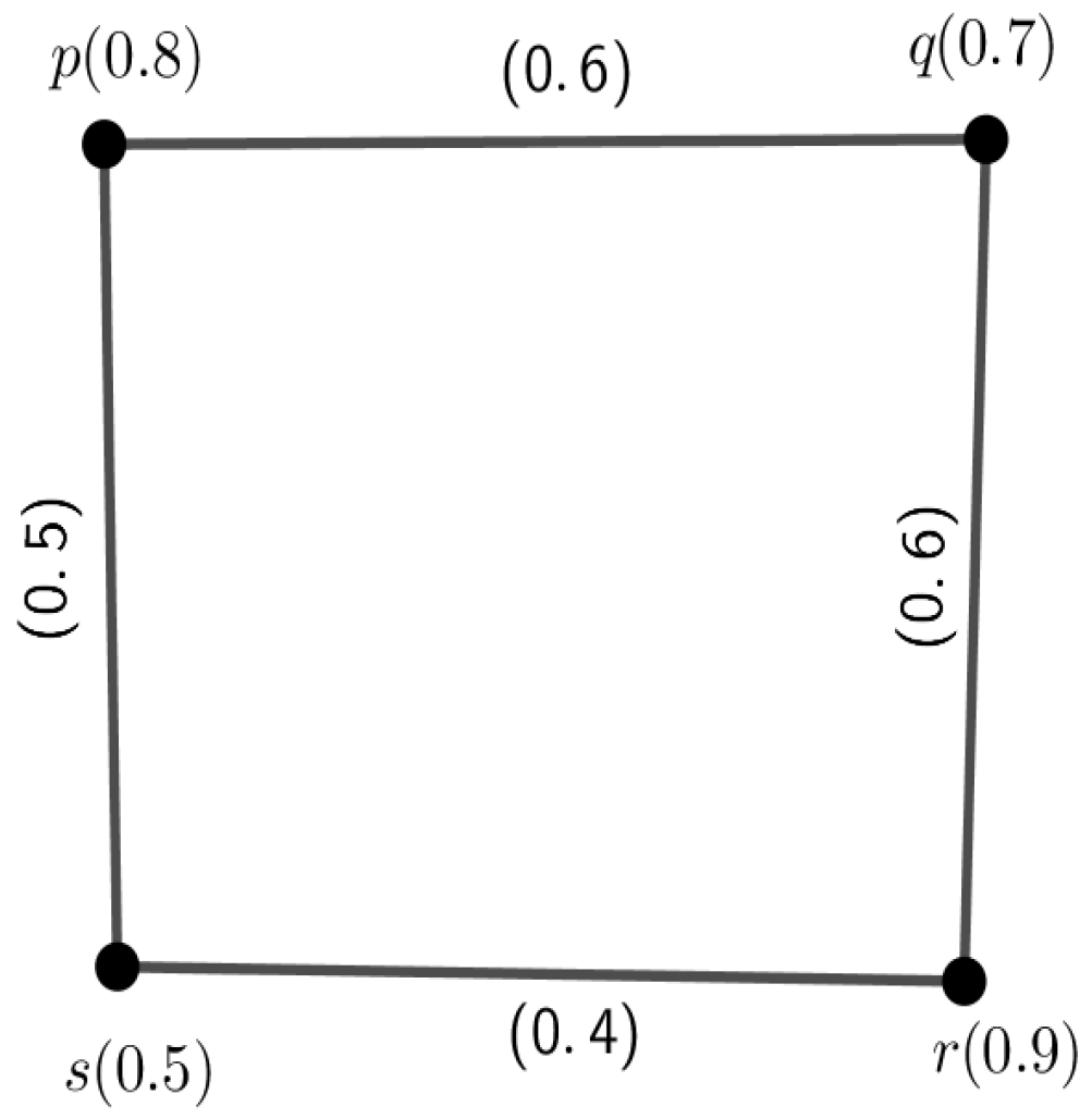
. The graph of K where the edge is deleted from G is shown in Figure 5.
From this figure,
Now,
.
This shows that
- .
- .
Theorem 4.
Let G be an FG and H be an FSG of then .
Proof.
Since is an FSG of , therefore
for all vertices x and for all edges e. This sows that for all vertices x.
Additionally, for all edges e, where d and represent the degrees of G and H. Now,
Hence, . □
Theorem 5.
Let be an FG and be the corresponding MST of G then .
Proof.
Since is an MST of therefore F is an FSG of G. Then we can say from the above Theorem, . □
Theorem 6.
Let G be an FG and let be an α cut FG of . Then, where the FG is defined as and , for all .
Proof.
Since is an FSG of the FG G, then by the above Theorem, . □
Theorem 7.
Let G be an FG and let Then .
Proof.
Since , therefore is a PFSG of . Then, by the above Theorem, . □
Corollary 1.
Let G be an FG and let .
Then, .
Theorem 8.
Let be a path. Then,
- .
- .
Proof.
Given that is a path, there are vertices and n edges.
- Now,Here, the degree of each vertex , except and , is and the degree of is and degree of is .Additionally, the degree of each edge , except and , is and the degree of is , the degree of is .Using this result, we have from ,
- From Equation , we get.As and ,(where ).So, .
□
Theorem 9.
Let be a path. If we take , it becomes a cycle . Then .
Proof.
Let d and denote the degree of a vertex/edge in G and H respectively. Here, for all vertices except and . Now, and and . Additionally, for all edges except and . Now, and and .
Now,
.
So, . □
Example 7.
Let G be a path with vertex set such that and shown in Figure 7.
Then,
Now,
.
Marge two vertex a and e in G, as shown in Figure 8.
Then,
Now,
.
Theorem 10.
Let be a cycle. Then,
- .
Proof.
Similar proof to Theorem 8. □
Theorem 11.
Let and be two fuzzy graphs and they are isomorphic to each other. Then, .
Proof.
As and are isomorphic to each other, then there exists a bijective mapping and for all then and
Then, .
Now,
.
So, □
Theorem 12.
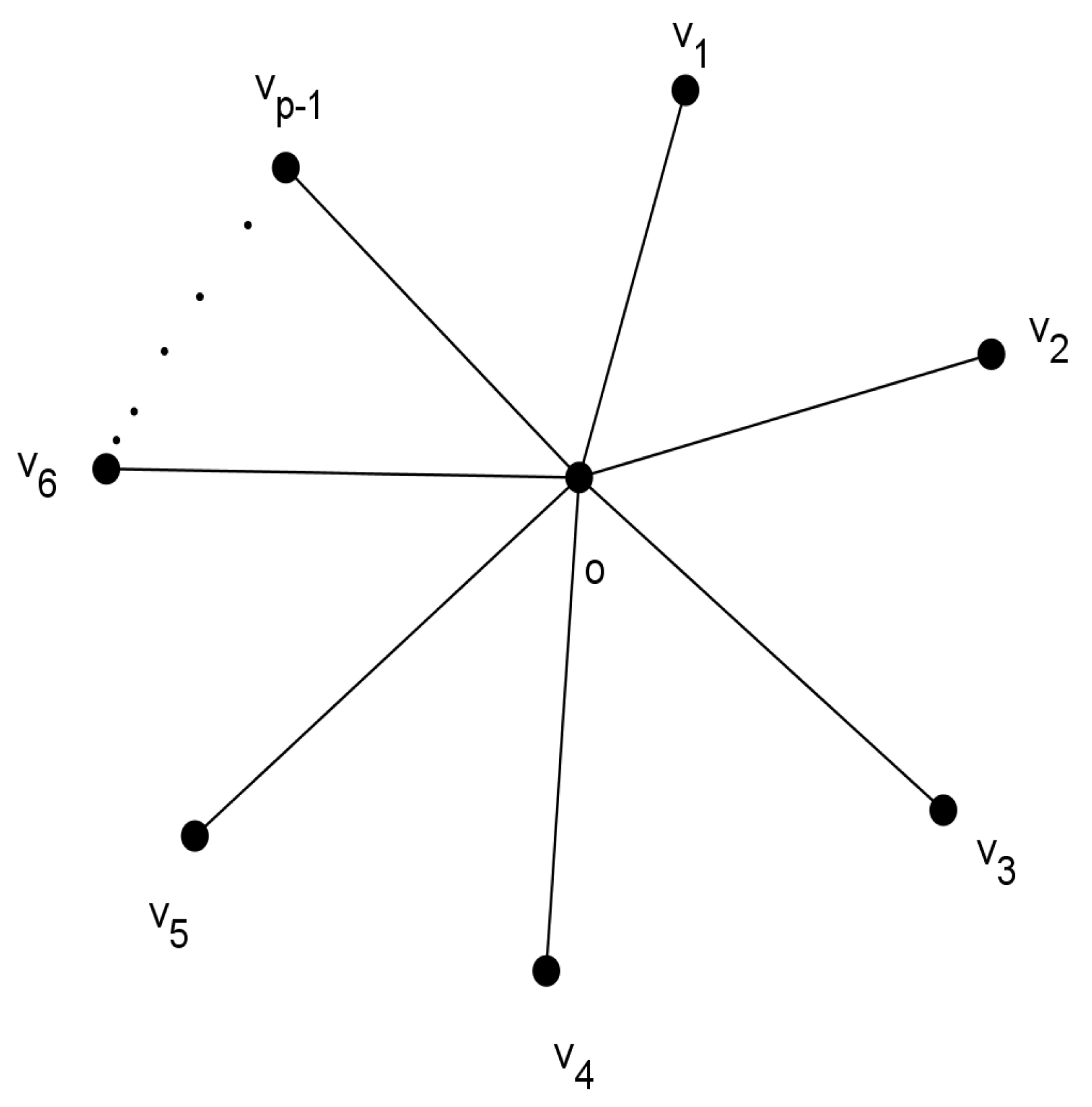
If (see Figure 9) is a star and satisfies the condition , where o is the center of the star, then the value of the FEZI is
.
Proof.
Given that , where o is the center of the star, so for all edges. Now, for all is given by and also .
Now,
.
This shows that . □
Theorem 13.
If is a double star, is the center of the first star and is the center of the second star and satisfies the condition for all , then .
Proof.
Since for all ,
.
Additionally, ,
,
.
Now,
. □
Theorem 14.
For a firefly graph , if the MV of each vertex as well as the edge is one, then the value of the FEZI is .
Proof.
Since the MV of each vertex and each edge is one, the number of vertices with degree 1 is ,
the number of vertices with degree 2 is ,
and ,
the number of edges with degree 1 is t,
the number of edges with degree 2 is s,
the remaining (p-t-1) edges have degree .
Then, the FEZI is
. □
Corollary 2.
If , then for a firefly graph,
If we put in , then the graph is a star similar to
So, .
4. Application of FEZI for Fuzzy Graphs to Find out the State Which Require More Development for Internet System
4.1. Model Construction
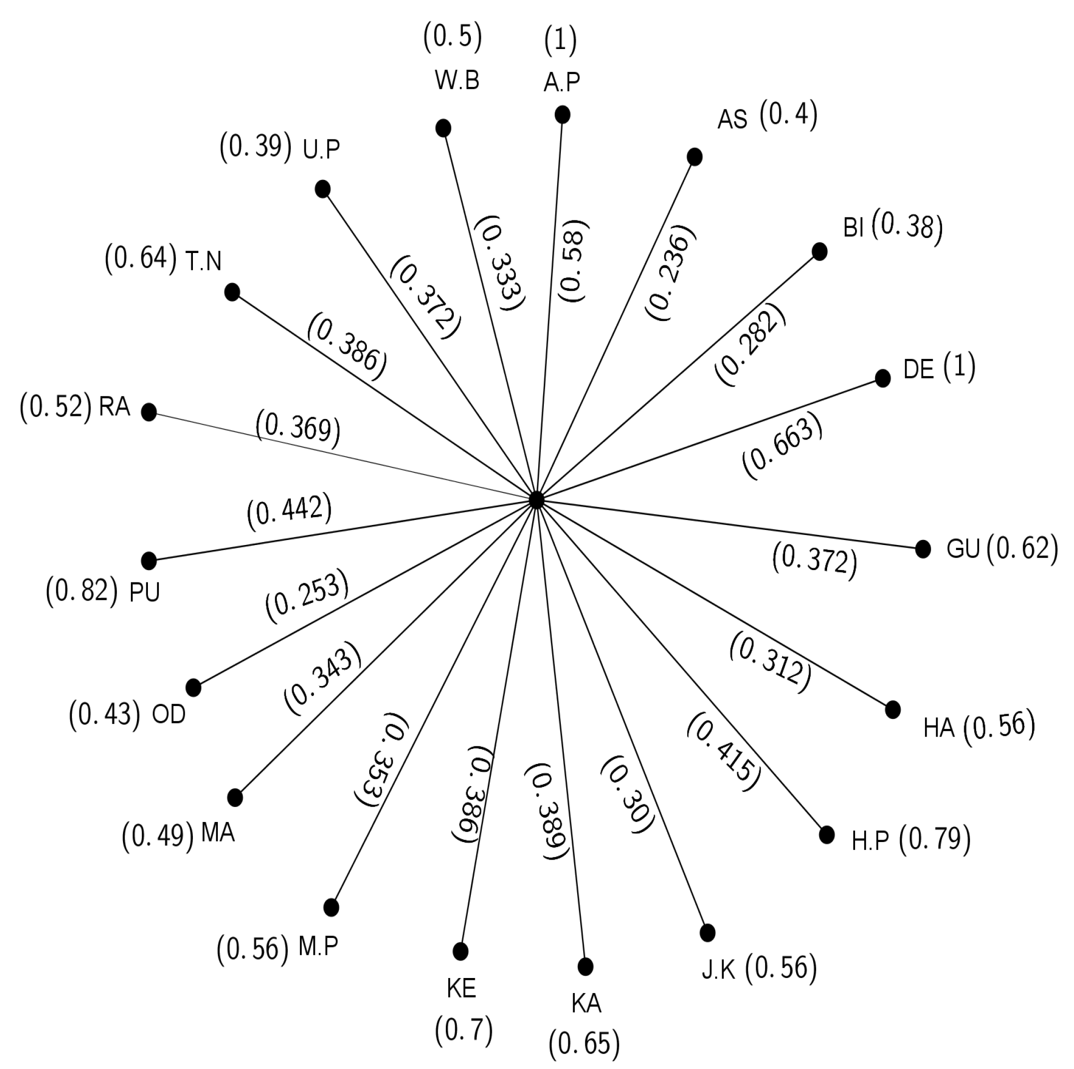
In the modern day, the internet is the most important part of our regular life. Here in this paper, we analyzed the Reliance Jio infocomm Ltd internet system in India. The data of Reliance Jio infocomm Ltd internet users are given in Table 1. These data were taken from https://dot.gov.in/sites/default/files/2022, accessed on 15 December 2022. Then, we constructed a Reliance Jio infocomm Ltd internet system graph (see Figure 10). Here, the whole graph is similar to a star where Reliance Jio infocomm Ltd (C) is the center of the star and each state is a pendent vertex of the star.
4.2. Representation of Membership Values
Now, the MV of a vertex is denoted as according to the formula below:
∧ {1,}.
Here we see that , since there is an edge between center C and a state S. The of this edge is denoted as and is defined by the following formula:
∧{1,}.
Here, we see that .
Then the value of the FEZI is given by
The FEZI of states (vertex) are given in the Table 4, and they are calculated by the formula .
4.3. Decision Making
From the Table 4, we have .
Now, the least FEZI of a vertex indicates that the vertex is most crucial for the development of internet network systems. Here, the first entire Zagreb index of two or more states is equal. In this situation, we will find the population percentage of these states who cannot use the internet. Then, the state having the largest population percentage that does not use the internet becomes the first to develop an internet network system.
Here, the percentages of the population who do not use the internet (PP) of the states are as follows: PP(AS) = 21.26, PP(BI) = 25.18, PP(OD) = 76.99, PP(HA) = 13.16, PP(J.K) = 6.05, PP(MA) = 64.38, PP(W.B) = 49.6, PP(M.P) = 37.82, PP(RA) = 38.45, PP(KA) = 23.62, PP(T.N) = 27.53. Then we can order the states as follows, and needing more development:
Odisha, Bihar, Assam, Uttar Pradesh, Maharashtra, West Bengal, Haryana, Jammu and Kashmir, Rajasthan, Madhya Pradesh, Gujrat, Tamil Nadu, Karnataka, Kerala, Himachal Pradesh, Punjab, Andhra Pradesh, Delhi.
5. Conclusions
In this article, the FEZI (first entire Zagreb index) was introduced as a graph parameter to quantify the structural characteristics of a graph. This study introduced several results and established relationships between various isomorphic graphs and -cut fuzzy graphs. Additionally, the paper provided bounds for some fuzzy graphs and applied these results to real-life problems in the field of internet system development. The precise values or boundaries of FEZI with regards to graphs such as the firefly graph, star, path, cycle, and others, were explored in this study. The relationship between the value of the FEZI of a graph and its subgraph, two isomorphic graphs, and the first Zagreb index and FEZI were also described here. To analyze the Reliance Jio infocomm Ltd. internet system in India, this paper constructed an internet system graph. In this graph, the least FEZI of a vertex indicates that the vertex is most crucial for the development of the internet network system, and the first entire Zagreb index of two or more states is equal. According to this paper, the state with the highest proportion of people who do not use the internet is the first to develop an internet network system. The first entire Zagreb index is also important in biochemistry, chemical graph theory, spectral graph theory, etc.
Author Contributions
Conceptualization, U.J. and G.G.; methodology, U.J. and G.G.; validation, U.J. and G.G.; formal analysis, U.J. and G.G.; investigation, U.J. and G.G.; data curation, U.J. and G.G.; writing—original draft preparation, U.J. and G.G.; writing—review and editing, U.J. and G.G.; visualization, U.J. and G.G.; supervision, U.J. and G.G.; project administration, U.J. and G.G.; funding acquisition. All authors have read and agreed to the published version of the manuscript.
Funding
The UGC of the Government of India is appreciative of the financial assistance under UGC-Ref. No.:201610294524 (CSIR-UGC NET NOVEMBER 2020) dated 01/04/2021.
Institutional Review Board Statement
Not applicable.
Informed Consent Statement
Not applicable.
Data Availability Statement
The data sets used and/or analyzed during the current study are available from the corresponding author on reasonable request.
Acknowledgments
The authors would like to express their sincere gratitude to the anonymous referees for valuable suggestions, which led to great deal of improvement of the original manuscript.
Conflicts of Interest
The authors declare no conflict of interest.
References
- Rosenfeld, A. Fuzzy Graph. In Fuzzy Sets and Their Applications; Zadeh, L.A., Fu, K.S., Shimura, M., Eds.; Academic Press: New York, NY, USA, 1975; pp. 77–95. [Google Scholar]
- Zadeh, L.A. Fuzzy Sets. Inf. Control 1965, 8, 338–353. [Google Scholar] [CrossRef]
- Yeh, R.T.; Bang, S.Y. Fuzzy relations. In Fuzzy Sets and Their Applications to Cognitive and Decision Process; Academic Press: New York, NY, USA, 1975; pp. 125–149. [Google Scholar]
- Sunitha, M.S.; Vijayakumar, A. A characterisation of fuzzy trees. Inf. Sci. 1999, 113, 293–300. [Google Scholar] [CrossRef]
- Sunitha, M.S.; Vijayakumar, A. Blocks in fuzzy graphs. J. Fuzzy Math. 2005, 13, 13–23. [Google Scholar]
- Mordeson, J.N.; Mathew, S. Advanced Topics in Fuzzy Graph Theory; Springer: Berlin, Germany, 2019; Volume 375. [Google Scholar]
- Al Mutab, H.M. Fuzzy Graphs. J. Adv. Math. 2019, 17, 77–95. [Google Scholar] [CrossRef]
- Bhutani, K.R. On automorphisms of fuzzy graphs. Pattern Recognit Lett. 1989, 9, 159–162. [Google Scholar] [CrossRef]
- Binu, M.; Mathew, S.; Mordeson, J.N. Wiener index of a fuzzy graph and application to illegal immigration networks. Fuzzy Sets Syst. 2020, 384, 132–147. [Google Scholar]
- De, N.; Nayeem, S.M.A.; Pal, A. Reformulated First Zagreb index of Some Graph Operations. Mathematics 2015, 3, 945–960. [Google Scholar] [CrossRef]
- Hosamani, S.M.; Basavanagoud, B. New upper bounds for the first Zagreb index. MATCH Commun. Math. Comput. Chem. 2015, 74, 97–101. [Google Scholar]
- Ghorai, G. Characterization of regular bipolar fuzzy graphs. Afr. Mat. 2021, 32, 1043–1057. [Google Scholar] [CrossRef]
- Ghorai, G.; Pal, M. Novel concepts of strongly edge irregular m-polar fuzzy graphs. Int. J. Appl. Comput. Math. 2016, 3, 3321–3332. [Google Scholar] [CrossRef]
- Islam, S.R.; Pal, M. First Zagreb index on a fuzzy graph and its application. J. Intell. Fuzzy Syst. 2021, 40, 10575–10587. [Google Scholar] [CrossRef]
- Poulik, S.; Ghorai, G. Determination of journeys order based on graphs Wiener absolute index with bipolar fuzzy information. Inf. Sci. 2021, 545, 608–619. [Google Scholar] [CrossRef]
- Gutman, I.; Trinajstic, N. Graph theory and molecular orbitals. Total ϕ-electron energy of alternate hydrocarbons. Chem. Phys. Lett. 1972, 17, 535–538. [Google Scholar] [CrossRef]
- Alwardi, A.; Alqesmah, A.; Rangarajan, R.; Cangul, I.N. Entire Zagreb indices of graphs. Discret. Math. Algorithms Appl. 2018, 10, 1850037. [Google Scholar] [CrossRef]
Figure 1.
A fuzzy graph.

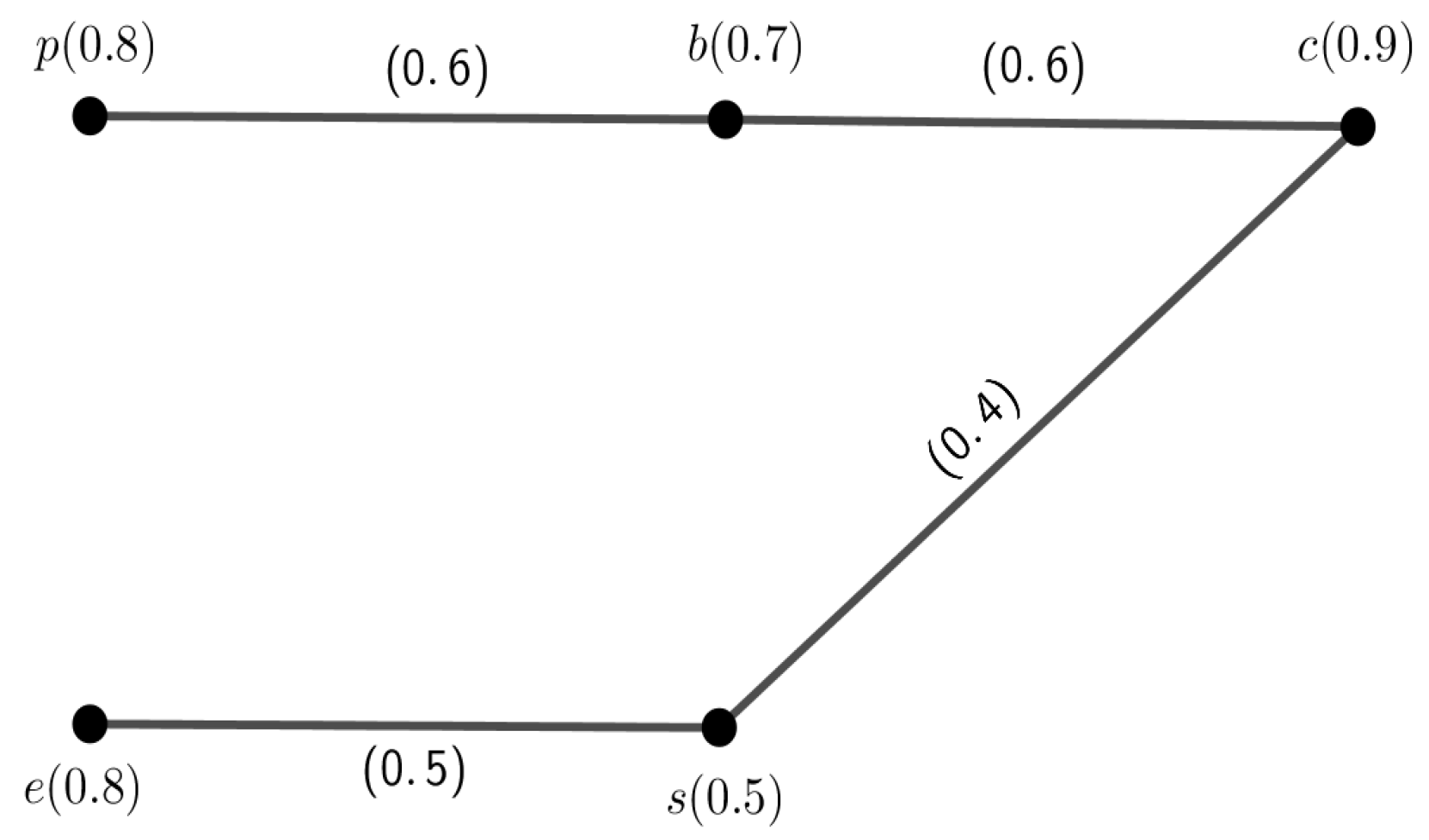
Figure 3.
A fuzzy graph G with = 3.6458.

Figure 4.
The FG obtained by deleting the vertex p from the above graph.

Figure 5.
The FG obtained by deleting an edge from the graph in Figure 3.
Figure 5.
The FG obtained by deleting an edge from the graph in Figure 3.

Figure 6.
A fuzzy path G with .

Figure 7.
A fuzzy path G with = 2.8317.

Figure 8.
A fuzzy graph H with .

Figure 9.
Graph of .

Figure 10.
Fuzzy graph of internet network of Reliance jio.


Table 1.
Data of internet users for all states.
| State | Internet Users (in Million) | Total Population (in Million) | Population Percentage of the State |
|---|---|---|---|
| Andhra Pradesh (A.P) | 56.06 | 52.883 | 4 |
| Assam (AS) | 14.14 | 35.4 | 2.6 |
| Bihar (BI) | 48.11 | 125.1 | 9.2 |
| Delhi (DE) | 38.89 | 31.2 | 2.3 |
| Gujrat (GU) | 43.68 | 70.7 | 5.2 |
| Haryana (HA) | 16.74 | 29.9 | 2.2 |
| Himachal Pradesh (H.P) | 5.89 | 7.45 | 0.50 |
| Jammu and Kashmir (J.K) | 7.55 | 13.6 | 1.0 |
| Karnataka (KA) | 43.68 | 67.3 | 4.9 |
| Kerala (KE) | 24.92 | 35.4 | 2.6 |
| Madhya Pradesh (M.P) | 47.78 | 85.6 | 6.3 |
| Maharashtra (MA) | 61.12 | 125.5 | 9.3 |
| Odisha (OD) | 19.02 | 44.2 | 3.3 |
| Punjab (PU) | 25.1 | 30.6 | 2.2 |
| Rajasthan (RA) | 41.75 | 80.2 | 5.9 |
| Tamil Nadu (T.N) | 49.17 | 76.7 | 5.6 |
| Uttar Pradesh (U.P) | 91.35 | 233.4 | 17.2 |
| West Bengal (W.B) | 49.1 | 98.7 | 7.3 |
Table 2.
Some values with respect to internet users.
| State | Jio Internet Users (Million) | |||
|---|---|---|---|---|
| A.P | 28.9 | 1.06 | 0.54 | 0.58 |
| AS | 7.3 | 0.4 | 0.21 | 0.236 |
| BI | 24.82 | 0.38 | 0.19 | 0.282 |
| DE | 20.06 | 1.25 | 0.64 | 0.663 |
| GU | 22.53 | 0.62 | 0.32 | 0.372 |
| HA | 8.64 | 0.56 | 0.29 | 0.312 |
| H.P | 3.03 | 0.79 | 0.41 | 0.415 |
| J.K | 3.89 | 0.56 | 0.29 | 0.30 |
| KA | 22.53 | 0.65 | 0.34 | 0.389 |
| KE | 12.86 | 0.70 | 0.36 | 0.386 |
| M.P | 24.65 | 0.56 | 0.29 | 0.353 |
| MA | 31.54 | 0.49 | 0.25 | 0.343 |
| OD | 9.81 | 0.43 | 0.22 | 0.253 |
| PU | 12.95 | 0.82 | 0.42 | 0.442 |
| RA | 21.54 | 0.52 | 0.27 | 0.369 |
| T.N | 25.37 | 0.64 | 0.33 | 0.386 |
| U.P | 47.13 | 0.39 | 0.20 | 0.372 |
| W.B | 25.34 | 0.5 | 0.26 | 0.333 |
Table 3.
Membership values and degrees of the FG of Figure 10.
Table 3.
Membership values and degrees of the FG of Figure 10.
| State | MV of the State (Vertex) | Degree of the State (Vertex) = MV of the Edge | Degree of an Edge between State and Center of the Star |
|---|---|---|---|
| A.P | 1 | 0.58 | 6.060 |
| AS | 0.4 | 0.236 | 6.550 |
| BI | 0.38 | 0.282 | 6.504 |
| DE | 1 | 0.663 | 6.123 |
| GU | 0.62 | 0.372 | 6.414 |
| HA | 0.56 | 0.312 | 6.474 |
| H.P | 0.79 | 0.415 | 6.371 |
| J.K | 0.56 | 0.30 | 6.486 |
| KA | 0.65 | 0.389 | 6.397 |
| KE | 0.70 | 0.386 | 6.400 |
| M.P | 0.56 | 0.353 | 6.433 |
| MA | 0.49 | 0.343 | 6.443 |
| OD | 0.43 | 0.253 | 6.533 |
| PU | 0.82 | 0.442 | 6.344 |
| RA | 0.52 | 0.369 | 6.417 |
| T.N | 0.64 | 0.386 | 6.400 |
| U.P | 0.39 | 0.372 | 6.414 |
| W.B | 0.5 | 0.333 | 6.453 |
Table 4.
Value of first entire Zagreb index for all states.
| State | ||
|---|---|---|
| A.P | 111.68 | 0.34 |
| AS | 112.01 | 0.01 |
| BI | 112.01 | 0.01 |
| DE | 111.58 | 0.44 |
| GU | 111.97 | 0.05 |
| HA | 111.99 | 0.03 |
| H.P | 111.91 | 0.11 |
| J.K | 111.99 | 0.03 |
| KA | 111.96 | 0.06 |
| KE | 111.95 | 0.07 |
| M.P | 111.98 | 0.04 |
| MA | 111.99 | 0.03 |
| OD | 112.01 | 0.01 |
| PU | 111.89 | 0.13 |
| RA | 111.98 | 0.04 |
| T.N | 111.96 | 0.06 |
| U.P | 112.00 | 0.02 |
| W.B | 111.99 | 0.03 |
Disclaimer/Publisher’s Note: The statements, opinions and data contained in all publications are solely those of the individual author(s) and contributor(s) and not of MDPI and/or the editor(s). MDPI and/or the editor(s) disclaim responsibility for any injury to people or property resulting from any ideas, methods, instructions or products referred to in the content. |
© 2023 by the authors. Licensee MDPI, Basel, Switzerland. This article is an open access article distributed under the terms and conditions of the Creative Commons Attribution (CC BY) license (https://creativecommons.org/licenses/by/4.0/).
Share and Cite
MDPI and ACS Style
Jana, U.; Ghorai, G. First Entire Zagreb Index of Fuzzy Graph and Its Application. Axioms 2023, 12, 415. https://doi.org/10.3390/axioms12050415
AMA Style
Jana U, Ghorai G. First Entire Zagreb Index of Fuzzy Graph and Its Application. Axioms. 2023; 12(5):415. https://doi.org/10.3390/axioms12050415
Chicago/Turabian StyleJana, Umapada, and Ganesh Ghorai. 2023. "First Entire Zagreb Index of Fuzzy Graph and Its Application" Axioms 12, no. 5: 415. https://doi.org/10.3390/axioms12050415
Note that from the first issue of 2016, this journal uses article numbers instead of page numbers. See further details here.