Stability of Anisotropy Pressure in Self-Gravitational Systems in $\mathit{f}\left(\mathcal{G}\right)$ Gravity

Abstract

This investigation aims to explore certain variables which are considered responsible for generating pressure anisotropy in dynamical spherically symmetric stellar systems against the background of the stringy-inspired Gauss–Bonnet modification of general relativity. We explore the hydrostatic equilibrium of self-gravitating systems by taking into account the modified form of Tolman–Oppenheimer–Volkoff for the quadratic-$f\left(\mathcal{G}\right)$ gravitational model. In this respect, we formulate a differential equation in terms of the Weyl curvature scalar, also described as an evolution equation, which is essential for understanding the evolution of the stellar structure. Finally, we conclude that the existence of some fluid variables such as shear, heat flux and the irregular behavior of energy density in the presence of an extra degree $f\left(\mathcal{G}\right)$-terms in the fluid flow that are the elements that cause anisotropy in the initially isotropic stellar structure. The comparison of the presented results with those of the classical model shows that they are physically relevant and compatible.

1. Introduction

In recent times, researchers devoted considerable attention to modified gravitational theories (MGT): specifically, on their interesting character in understanding accelerated cosmic expansion. One appealing aspect of higher-curvature MGT is that they can contribute to illustrating the inflationary mechanism of the universe by adding geometrical quantities in the usual Einstein–Hilbert action (EHA) [1,2] without the inclusion of a scalar field or dark energy (DE). The Gauss-Bonnet (GB) curvature scalar is

$$\begin{array}{c}\hfill \mathcal{G}={\mathbf{R}}^2+R_{\mu \upsilon \sigma \eta }{R}^{\mu \upsilon \sigma \eta }-R_{\mu \upsilon }{R}^{\mu \upsilon },\end{array}$$

(1)

where, $\mathbf{R}$ corresponds to the Ricci scalar, while $R_{\mu \upsilon }$ and $R_{\mu \upsilon \sigma \eta }$ denote the Ricci and Riemann tensors, respectively. This curvature invariant arises in the re-normalization of an intriguing quantum theory of fields in the curved spacetimes and plays a significant role in this perspective. Further, it should be pointed out that the scalar invariant $\mathcal{G}$ also emerges in the low energy actions of certain notable theories [3]. This work is devoted to analyzing the interesting results of an increasingly popular modified $f\left(\mathcal{G}\right)$ gravity [4], with gravitation lagrangian ${\mathcal{L}}_{f\left(\mathcal{G}\right)}=\mathbf{R}+f\left(\mathcal{G}\right)$. It is notable that, in four dimensions, $\mathcal{G}$ is referred to as a topological invariant. However, it may provide several captivating cosmological consequences in higher dimensions [5] and naturally arises in the string theories [6]). Further, it is demonstrated that certain realistic variants of the $f\left(\mathcal{G}\right)$ cosmological models are compatible with all the tests in the solar system.

It is significant to observe that the GB scalar curvature results from the unique incorporation of the square of curvature computing tensorial quantities such as ${\mathbf{R}}^2$, $R_{\mu \upsilon }{R}^{\mu \upsilon }$ and $R_{\mu \upsilon \sigma \eta }{R}^{\mu \upsilon \sigma \eta }$. This unique combination gives rise to a modified GB cosmological model, commonly termed the $f\left(\mathcal{G}\right)$ theory of gravitation. This cosmological model is exceptionally appealing for understanding the phenomenon of DE and the cosmological expansion [4].

• This modification of gravity is conformal with the standard tests of our solar system and presents a natural substitute for gravitational DE [7,8].
• This gravitational alternative may be utilized for explaining the unified description of dark matter as well as DE. Some of the important cosmological consequences such as rotational curves of spiral galaxies may also be studied successfully in $f\left(\mathcal{G}\right)$-gravity.
• During cosmic evolution, it naturally illustrates the transition from deceleration to an acceleration of the cosmic era [9].
• This gravitational model can describe the cosmic transition from the non-phantom to the phantom phase, without the inclusion of any exotic matter [10]. It is observed that the phantom era appears to be in this modification, thereby avoiding the happening of Big Rip.
• It is expected that this alternative gravity can be utilized with the assistance of effective DE dominance. Therefore, the problem of coincidence can also be resolved naturally by the phenomena of cosmic speed-up.
• This form of gravity model can also be advantageous in the field of high energy physics, such as for the justification of hierarchy problem [11] and for the unification of gravity with grand unified theories. However, it is important to note that the above-stated features are possible for some specific models, but not exhibited by all $f\left(\mathcal{G}\right)$ models.

The framework of the GB-gravitational model is interesting for numerous reasons, including the preservation of significant aspects of the gravitational theory, such as diffeomorphism invariance, Bianchi identities, and second-order quasi-linear gravitational field equations. The presence of GB correction in the standard EHA action is a useful scheme for curing the shortcomings associated with $f\left(\mathbf{R}\right)$-gravity such as the existence of ghosts [12]. Moreover, Flaut and Shpakivskyi [13] described that some functions of the GB quantity are linked to the conserved quantities. The GB combination of squared-curvature terms can avoid the emergence of pseudo-spin-2 ghosts [14,15,16], and is also useful in ruling out the matter instabilities [17], regardless of the fact that they are consistent with local gravitational restrictions as well as late-time cosmic acceleration. Additionally, the GB-cosmology is considered one of the interesting cosmological models to cure finite-time future singularities [18] and is also beneficial in regularizing the standard EHA-action.

In relativistic astrophysics, compact stars are produced through a significant gravitational process called the gravitational collapse of highly dense and massive stellar systems. The small size and enormously massive framework of the stellar systems result in very strong gravitational interactions. The physical characteristics of compact stars involve certain relationships between the force of gravity and the interior pressure of stellar structure that gives rise to the equilibrium state, commonly characterized as hydrostatic equilibrium. This phenomenon plays a crucial role in studying interior stellar structures. The solutions for compact stars are often illustrated through hydrostatic equilibrium equations or Tolman–Oppenheimer–Volkoff (TOV) equations. In the field of gravitational physics and modern relativistic astrophysics, the investigation of compact stellar objects has gained particular interest due to their massive structure and interesting features.

Initially, Gamow [19] discussed the transition of neutron stars and computed the critical mass of neutron stars using homogenous matter configurations, as formerly attempted by Stoner [20], for white dwarfs. Gamow’s conception was concerned with the comparison of Newtonian gravitational pressures and ultra-relativistic pressures. Chandrasekhar [21,22] calculated the maximal mass of white dwarfs and also discussed their stability and evolution. Oppenheimer and Volkoff [23] proposed that a new phase composed of neutrons will form when the pressure inside stellar matter reaches a certain level. It is notable that the first consistent neutron star model involving internal energy contributions was developed by Tolman, Oppenheimer and Volkof. Moreover, Oppenheimer and Snyder [24] performed a comprehensive study on the continued gravitational contraction. Several studies have been performed to explore the dynamics of compact stellar objects using TOV equations [25,26,27,28,29]. The TOV equations provide significant correspondence between certain physical quantities such as mass, pressure, and energy density of a specific stellar structure. In addition, TOV equations enable us to calculate the deviations of the stellar pressure and energy density related to the mass of compact self-gravitational system.

Pani et al. [30] developed a formalism to study the self-gravitational structure by considering the GB-corrections. Moreover, they analyzed the stability and existence of compact stars in quadratic curvature corrections. The presence of quadratic GB-corrections $\left(\alpha {\mathcal{G}}^2\right)$ enables us to obtain stable stellar configurations with high central densities for $\alpha <0$, as observed in the case of neutron star [25]. The radii and the masses of the corresponding stellar systems differ from classical general relativity (GR) inconsiderably, since the quadratic term ${\mathcal{G}}^2$ is small as compared to the $\mathbf{R}$ term. However, the nature of mass density dependence alters. In a small range of densities, the mass tends to grow as the central density rises. Bhar et al. [31] executed a comparative study regarding the dynamics of compact stars in both GR and GB-gravity. They discussed that the values of density and pressure are higher in the case of the GB star model than in the GR model. There are some reviews on the study of $f\left(\mathcal{G}\right)$ gravity [32,33] which describe the implication of $f\left(\mathcal{G}\right)$ gravity on a few cosmic puzzles.

The GB curvature scalar is shown to be a conserved topological invariant when integrated into four-dimensional spacetime; its addition to the EHA action has no contribution to the gravitational dynamics. However, a non-minimal coupled configuration of GB-scalar induces some salient characteristics as an alternative to gravitational DE. More recently, Glavan and Lin [34] suggested a generic four-dimensional GB-gravitational theory and found that the GB-term produces non-trivial gravitational effects in four dimensions. The central theme of their investigation was the rescaling of the GB curvature scalar by $\alpha \to \alpha /(D-4)$ in a D-dimensional manifold, under the limit D$\to \alpha$. Silva et al. [35] observed that compact stars manifest spontaneous scalarization in GB-gravity. Most recently, Nashed et al. [36] studied the characteristics of anisotropic compact systems using TOV equations in the limit of $D\to 4$. Oikonomou [37] explored certain solutions representing singular cosmological bounce having type-IV singularity at the bouncing point, using $f\left(\mathcal{G}\right)$ gravity. Bruck and Longden extended the notion of Higgs inflation [38] and studied a few realistic inflationary models during reheating [39], with the help of GB-coupling. Makarenko and Myagky [40] considered a $f\left(\mathcal{G}\right)$ gravitational model to analyze the bouncing nature that existed in the early-time universe and provided some asymptotic solutions for this model. Santillán [41] investigated certain homogeneous and isotropic models without potential via a four-dimensional GB model. Tariq et al. [42] pointed out certain elements responsible for the emergence of anisotropy of self-gravitating systems through the principles of Palatini $f\left(\mathbf{R}\right)$-corrections. Bhatti and Yousaf [43] studied the instability bounds for spherically charged self-gravitational systems for the $f\left(\mathcal{G}\right)$-corrections. Bhatti et al. [44,45] investigated the quasi-homologous evolution of charged and uncharged complex self-gravitational fluids within the dynamics of GB-cosmology.

In this endeavor, we have generalized Herrera’s work [46] to formulate the stability condition for isotropic pressure through the mechanism of a GB-cosmological model. This investigation is mainly concerned with finding a solution to the following issues:

• What material characteristics of the considered fluid configuration are responsible for changing the behavior of the fluid configuration from isotropic to anisotropic?
• What circumstances cause an originally isotropic distribution to remain isotropic throughout its evolution?

The overview of the manuscript is described as follows: In Section 2, we review the standard formalism of modified $f\left(\mathcal{G}\right)$ cosmology, equations of motion, gravitational mass, as well as the corresponding TOV equations for the quadratic GB corrections. In Section 3, we explore a significant differential equation in terms of Weyl curvature scalar by constructing significant relations between pressure anisotropy, energy density as well as geometric and dissipative variables. In Section 4, we discuss in detail the necessary condition for the existence of pressure anisotropy along with the evolution of the self-gravitational structure. We also identify the physical factors that are responsible for the departure from this condition in the same section. In Section 5, we formulate the mass–radius diagrams for the $\mathcal{G}+\alpha {\mathcal{G}}^2$ gravity model. Finally, the conclusion is drawn in Section 5.

2. Tolman–Oppenheimer–Volkoff Equations in $\mathit{f}\left(\mathcal{G}\right)$ Gravity

The standard gravitational action in the context of $f\left(\mathcal{G}\right)$ cosmological model was initially proposed in [4] as

$$\begin{array}{c}\hfill S_{f\left(\mathcal{G}\right)}\equiv S_{\mathrm{G}}+S_{\mathrm{M}}=\int \left(\frac{1}{2{\kappa }^2}\mathbf{R}+f\left(\mathcal{G}\right)\right)\sqrt{-g}{d}^{4}x+\int {\mathcal{L}}_m\sqrt{-g}{d}^{4}x,\end{array}$$

(2)

where $S_{\mathrm{G}}$ and $S_{\mathrm{M}}$ are the gravitational and matter actions, respectively. Moreover, $\mathbf{R}$ is the curvature scalar and g = det($g_{\mu \upsilon }$), ${\kappa }^2$ is the coupling constant and ${\mathcal{L}}_m$ symbolizes the density of matter Lagrangian. In our calculations, we choose the units such that ${\kappa }^2\equiv 8\pi \tilde{G}$ = 1, and $\tilde{G}$ denotes the Newtonian constant. Furthermore, f is a generic differentiable function of the GB scalar, $\mathcal{G}$, which is a total differential in four dimensions. Hence, the GB-equations remain invariant under the choice of $f\left(\mathcal{G}\right)=\mathcal{G}$. However, for other functional forms, this factor makes non-trivial effects to the equations of motion.

Thus, upon varying the gravitational action (2) w.r.t. $g^{\mu \upsilon }$, we obtain

$$\begin{array}{cc}\hfill G_{\mu \upsilon }& +4\left[R_{\mu \sigma \upsilon \eta }+R_{\sigma \upsilon }{g}_{\mu \eta }-R_{\sigma \eta }{g}_{\upsilon \mu }-R_{\mu \upsilon }{g}_{\sigma \eta }+R_{\mu \eta }{g}_{\upsilon \sigma }\right.\hfill \\ \hfill & +\left.\frac{\mathbf{R}}{2}(g_{\mu \upsilon }{g}_{\sigma \eta }-g_{\mu \eta }{g}_{\upsilon \sigma })\right]{\nabla }^{\upsilon }{\nabla }^{\sigma }{f}_{\mathcal{G}}+\frac{1}{2}(\mathcal{G}{f}_{\mathcal{G}}-f)g_{\mu \upsilon }=T_{\mu \upsilon },\hfill \end{array}$$

(3)

where $f_{\mathcal{GG}\cdots }=\frac{d^{n}f\left(\mathcal{G}\right)}{d{\mathcal{G}}^n}$. The higher-order $f\left(\mathcal{G}\right)$ gravity terms emerging in the above equation can be advantageous in exploring the inflationary, as well as the acceleratory mechanism of our universe. Here, ${\nabla }_{\sigma }$ is an operator used for covariant differentiation. Moreover, the tensorial quantities $G_{\mu \upsilon }$ and $T_{\mu \upsilon }$ represent the Einstein tensor and usual stress–energy tensor, respectively.

$$\begin{array}{c}\hfill T_{\mu \upsilon }=\rho V_{\mu }{V}_{\upsilon }+{\mathrm{\Pi }}_{\mu \upsilon }+P{h}_{\mu \upsilon }+({\chi }_{\mu }{V}_{\upsilon }+{\chi }_{\upsilon }{V}_{\mu })q.\end{array}$$

(4)

where in this equation, $q=q(t,r)$ is the magnitude of the heat flux, P represents the fluid’s pressure, $\rho$ denotes the energy-density and $V_{\mu }$ stands for the four-velocity vector. For comoving coordinates, these quantities follow the following relationships

$$\begin{array}{c}\hfill V_{\mu }{\chi }^{\mu }=0,q_{\mu }{V}^{\mu }=0,{\chi }_{\mu }{\chi }^{\mu }=1,V_{\mu }{V}^{\mu }=-1.\end{array}$$

(5)

In addition, ${\mathrm{\Pi }}_{\mu \upsilon }$ is the anisotropic pressure tensor, which can be defined via unit four-vector ${\chi }_{\mu }$ and projection tensor $h_{\mu \upsilon }$ as

$$\begin{array}{c}\hfill {\mathrm{\Pi }}_{\mu \upsilon }=\mathrm{\Pi }\left({\chi }_{\mu }{\chi }_{\upsilon }-\frac{1}{3}{h}_{\mu \upsilon }\right),\mathrm{where}{h}_{\mu \upsilon }=V_{\mu }{V}_{\upsilon }+g_{\mu \upsilon },\end{array}$$

(6)

where $\mathrm{\Pi }\equiv P_r-P_{\perp }$, with $P_r$ and $P_{\perp }$ being pressure components along the radial and transverse directions, respectively.

The investigations on anisotropic compact stars consistently remained a subject of growing attention in the field of relativistic astrophysics. Generally, the anisotropy in compact stellar systems arises due to the existence of combinations of several types of fluid distributions, such as rotation, the existence of the external fields, the presence of superfluid [47] and phase transitions. When densities associated with gravitational systems are normally higher than the particular nuclear-matter density, the pressure is split into two distinct constituents i.e., $P_r$ and $P_{\perp }$. This fact gives rise to the anisotropic condition that $\left(P_r\right)$ is not equal to $\left(P_{\perp }\right)$. Therefore, in an anisotropic fluid configuration, the above-stated pressure components are unequal, i.e., $P_r\ne P_{\perp }$. This effect was suggested by Jeans [48] for self-gravitational systems. Later on, Lemaître [49] also studied the local anisotropy within the formalism of classical GR.

The anisotropic effects in understanding the framework and evolution of gravitational configurations were initially proposed by Bowers and Liang [50]. They formulated the modified form of hydrostatic equilibrium equation which includes the anisotropic effects, for spherically symmetric matter distributions in GR. In this respect, several studies are available in the literature [51,52]. Bhar et al. [53] studied anisotropic stellar objects models for spherically symmetric geometry and discussed various physical features corresponding to the compact objects. Maurya et al. [54] studied a family of relativistic stellar solutions for static spherically symmetric anisotropic fluids in hydrostatic equilibrium by using the Buchdahl ansatz.

The spherically symmetric solutions are considered to be the most significant tools in describing the physical characteristics and structure of isotropic, as well as anisotropic compact stellar objects, both in GR and MGT. Shamir [55] analyzed the dynamics of anisotropy in compact stellar configurations through the mechanism of different $f\left(\mathcal{G}\right)$ cosmological models. The same author discussed the dynamics of the anisotropic universe through the background of string-inspired $f\left(\mathcal{G}\right)$ gravity. He discussed the energy conditions and proved that the failure of strong energy conditions indicates the emergence of an anisotropic universe in this modified theory. Bhatti et al. [56] examined the evolution of relativistic compact objects such as neutron stars by constructing the TOV equations in the $f(\mathbf{R},T)$ cosmological model. Maurya et al. [54] investigated the dynamics of compact stellar systems under an anisotropic environment by assuming a time-independent spherically symmetric source. Nashed and Capozziello [57] investigated the dynamics of anisotropic compact objects by constructing some solutions corresponding to self-gravitational structure for $f\left(\mathbf{R}\right)$ cosmology. Mustafa et al. [58] formulated spherically symmetric solutions corresponding to three different anisotropic stellar systems for $f\left(\mathcal{G}\right)$ gravity. They investigated different features corresponding to the stellar systems by constructing the modified TOV equations.

Next, choosing comoving coordinates, the generic form of dynamical spherically symmetric metric is given as

$$\begin{array}{c}\hfill d{s}^2=-A^2(t,r)d{t}^2+B^2(t,r)d{r}^2+C^2(t,r)(d{\theta }^2+{sin}^2\theta d{\varphi }^2),\end{array}$$

(7)

where the spherical coordinates are labeled as $x^{\mu }=(t,r,\theta ,\varphi )$, with $\mu =0,1,2,3.$ In case of comoving observers, the above metric fulfills the following relationships:

$$\begin{array}{c}\hfill V^{\mu }=\frac{1}{A}{\delta }_0^{\mu },{\chi }^{\mu }=\frac{1}{B}{\delta }_1^{\mu },q^{\mu }=\frac{1}{B}q{\delta }_1^{\mu },\end{array}$$

(8)

where the heat flux vector q is a function of temporal as well as radial coordinates, i.e., $q=q(t,r)$.

The irrotational fluid distribution can be entirely discussed via three types of physical parameters, i.e., shear tensor $\left({\sigma }_{\mu \upsilon }\right)$, expansion scalar $\left(\mathrm{\Theta }\right)$ and four-acceleration $\left(a_{\mu }\right)$. The shear tensor is defined as

$$\begin{array}{c}\hfill {\sigma }_{\mu \upsilon }=V_{\mu ;\upsilon }+a_{(\mu }{V}_{\upsilon )}-\frac{1}{3}\mathrm{\Theta }{h}_{\mu \upsilon }.\end{array}$$

(9)

The non-vanishing constituents of the above equation are

$$\begin{array}{cc}\hfill {\sigma }_{11}& =\frac{2\sigma }{3}{B}^2,{\sigma }_{22}=\frac{{\sigma }_{33}}{{sin}^2\theta }=-\frac{\sigma }{3}{C}^2,\mathrm{where}\sigma =\frac{1}{A}\left(\frac{\dot{B}}{B}-\frac{\dot{C}}{C}\right),\hfill \end{array}$$

(10)

where $\sigma$ denotes the shear scalar and dot indicates t-derivative. The tensor ${\sigma }_{\mu \upsilon }$ can also be defined in terms of projection tensor and unit four vector as

$$\begin{array}{c}\hfill {\sigma }_{\mu \upsilon }=\sigma \left({\chi }_{\mu }{\chi }_{\upsilon }-\frac{1}{3}{h}_{\mu \upsilon }\right).\end{array}$$

(11)

On the other hand, $\mathrm{\Theta }$ and $a_{\mu }$ are defined as

$$\begin{array}{c}\hfill \mathrm{\Theta }=V_{;\mu }^{\mu },a_{\mu }=V_{\mu ;\upsilon }{V}^{\upsilon }.\end{array}$$

(12)

These variables are responsible for measuring the expansion and the influence of inertial forces on the fluid distribution, respectively. Their non-null components are defined as

$$\begin{array}{cc}\hfill \mathrm{\Theta }=\frac{1}{A}\left(2\frac{\dot{C}}{C}+\frac{\dot{B}}{B}\right),a_1=\frac{A^{\prime }}{A},a^{\mu }{a}_{\mu }& ={\left(\frac{A^{\prime }}{AB}\right)}^2,\mathrm{where}{a}^{\mu }{a}_{\mu }=a^2.\hfill \end{array}$$

(13)

Here, a denotes the four-acceleration scalar and prime indicates the r-derivative.

Next, the gravitational field equations for $f\left(\mathcal{G}\right)$ gravity, using Equations (4)–(7), are defined as

$$\begin{array}{cc}\hfill \rho & =\frac{1}{A^2}\left(\frac{\dot{C}}{C}+2\frac{\dot{B}}{B}\right)\frac{\dot{C}}{C}-\frac{1}{B^2}\left[{\left(\frac{C^{\prime }}{C}\right)}^2-{\left(\frac{B}{C}\right)}^2+\frac{2}{C}\left(C^{\prime \prime }+\frac{B^{\prime }}{B}{C}^{\prime }\right)\right]\hfill \\ & +{\varphi }_1{\dot{\mathcal{G}}}^2{f}_{\mathcal{GGG}}+({\varphi }_1\ddot{\mathcal{G}}+{\varphi }_2\dot{\mathcal{G}}+{\varphi }_3{\mathcal{G}}^{\prime })f_{\mathcal{GG}}-\frac{1}{2}(\mathcal{G}{f}_{\mathcal{G}}-f),\hfill \end{array}$$

(14)

$$q=\frac{2}{AB}\left(\frac{{\dot{C}}^{\prime }}{C}-\frac{A^{\prime }\dot{C}}{AC}-\frac{C^{\prime }\dot{B}}{CB}\right)+({\eta }_1\dot{\mathcal{G}}+{\eta }_2{\mathcal{G}}^{\prime }+{\eta }_3{\dot{\mathcal{G}}}^{\prime })f_{\mathcal{GG}},$$

(15)

$$\begin{array}{cc}\hfill P_r& =\frac{1}{B^2}\left(\frac{C^{\prime }}{C}+2\frac{A^{\prime }}{A}\right)\frac{C^{\prime }}{C}-\frac{1}{A^2}\left[2\frac{\ddot{C}}{C}+{\left(\frac{\dot{C}}{C}\right)}^2-2\frac{\dot{C}\dot{A}}{CA}\right]-\frac{1}{C^2}\hfill \\ & +{\phi }_1{\mathcal{G}}^{\prime }2f_{\mathcal{GGG}}+({\phi }_1{\mathcal{G}}^{″}+{\phi }_2{\mathcal{G}}^{\prime }+{\phi }_3\dot{\mathcal{G}})f_{\mathcal{GG}}+\frac{1}{2}(\mathcal{G}{f}_{\mathcal{G}}-f),\hfill \end{array}$$

(16)

$$\begin{array}{cc}\hfill P_{\perp }& =\frac{1}{B^2}\left[\frac{C^{″}}{C}+\frac{A^{″}}{A}-\frac{B^{\prime }{A}^{\prime }}{BA}-\left(\frac{B^{\prime }}{B}-\frac{A^{\prime }}{A}\right)\frac{C}{C^{\prime }}\right]-\frac{1}{A^2}\left[\frac{\ddot{C}}{C}+\frac{\ddot{B}}{B}\right.\hfill \\ & +\left.\frac{\dot{B}}{B}\left(\frac{\dot{C}}{C}-\frac{\dot{A}}{A}\right)-\frac{\dot{A}\dot{C}}{AC}\right]+({\psi }_1{\dot{\mathcal{G}}}^2+{\psi }_2{{\mathcal{G}}^{\prime }}^2+{\psi }_5\dot{\mathcal{G}}{\mathcal{G}}^{\prime })f_{\mathcal{GGG}}\hfill \\ & +({\psi }_1\ddot{\mathcal{G}}+{\psi }_2{\mathcal{G}}^{″}+{\psi }_3{\mathcal{G}}^{\prime }+{\psi }_4\dot{\mathcal{G}}+{\psi }_5{\dot{\mathcal{G}}}^{\prime })f_{\mathcal{GG}}+\frac{1}{2}(\mathcal{G}{f}_{\mathcal{G}}-f).\hfill \end{array}$$

(17)

where the values of the $f\left(\mathcal{G}\right)$-corrections ${\varphi }_i$, ${\phi }_i$ and ${\psi }_i$ ($i=1,2,\dots ,n$) are given in the appendix, as in Equations (A1)–(A15), respectively. The above-stated gravitational field equations can be reduced for classical GR, under usual limits. The hydrostatic equilibrium equation is obtained by contracting the Bianchi identities ${\nabla }_{\mu }{T}_{\upsilon }^{\mu }$ for $\upsilon =r$ as

$$\begin{array}{c}\hfill \frac{d{P}_r}{dr}=-(\rho +P_r)\frac{A^{\prime }}{A}+2(P_{\perp }-P_r)\frac{C^{\prime }}{C}.\end{array}$$

(18)

This result generalizes the TOV Equation [50] for the GR cosmological theory for anisotropic stellar systems. The above equation is satisfied identically for $\upsilon =t$.

We have used the definition of the Misner–Sharp (MS) mass function suggested in [59,60] as

$$\begin{array}{c}\hfill m(t,r)=\frac{C}{2}{R}_{232}^3,\end{array}$$

(19)

where $C=C(t,r)$ is the proper radius of the spherical star and $R_{232}^3$ is the component of the Riemann tensor. Zhang et al. [61] formulated the MS-mass function in n-dimensional $f\left(\mathbf{R}\right)$ gravitational theory. By following a similar procedure, Maeda [62] generalized the MS-mass function in the Einstein-GB gravitational model for the $n(\ge 5)$ dimensional metric. As we are working in the four-dimensional spacetime, the definition of MS-mass therefore remains similar to that of GR [59].

Thus, the geometric mass $m(t,r)$ of a spherically symmetric star can be written using MS formalism mentioned in Equation (19) as

$$\begin{array}{c}\hfill m(t,r)=\frac{C}{2}{R}_{232}^3=\frac{C}{2}\left[1-{\left(\frac{C^{\prime }}{B}\right)}^2+{\left(\frac{\dot{C}}{A}\right)}^2\right].\end{array}$$

(20)

Here, $\tilde{E}\equiv \frac{C^{\prime }}{B}={\left(1+U^2-\frac{2m}{C}\right)}^{\frac{1}{2}}$ and $U=\frac{\dot{C}}{A}$. Now the corresponding TOV equations can be obtained by writing the $f\left(\mathcal{G}\right)$ field equations in terms of $\frac{d{P}_r}{dr}$ and $D_C\left(m\right)=\frac{1}{C}\frac{dm}{dr}$. Then, after some manipulation, we obtain

$$\begin{array}{cc}\hfill D_C\left(m\right)& =\frac{1}{2}\left(\rho +q\frac{U}{\tilde{E}}\right)C^2+\frac{1}{2}{\varphi }_1{\dot{\mathcal{G}}}^2{f}_{\mathcal{GGG}}{C}^2+\frac{1}{2}\left[C^2\left({\varphi }_1\ddot{\mathcal{G}}+{\varphi }_2\dot{\mathcal{G}}+{\varphi }_3{\mathcal{G}}^{\prime }\right)\right.\hfill \\ \hfill & +\left.\frac{qU}{\tilde{E}}\left({\eta }_1\dot{\mathcal{G}}+{\eta }_2{\mathcal{G}}^{\prime }+{\eta }_3{\dot{\mathcal{G}}}^{\prime }\right)\right]f_{\mathcal{GG}}-\frac{1}{4}(\mathcal{G}{f}_{\mathcal{G}}-f)C^2,\hfill \end{array}$$

(21)

$$\begin{array}{cc}\hfill \frac{d{P}_r}{dr}=& -\left[\rho +P_r-\frac{1}{B^4}\left\{{\phi }_1{{\mathcal{G}}^{\prime }}^2{f}_{\mathcal{GGG}}+\left({\phi }_1{\mathcal{G}}^{″}+{\phi }_2{\mathcal{G}}^{\prime }+{\phi }_3\dot{\mathcal{G}}\right)\right\}\right.\hfill \\ \hfill +& \left.\frac{1}{A^2{B}^2}\left\{{\varphi }_1{\dot{\mathcal{G}}}_{\mathcal{GGG}}^2+\left({\varphi }_1\ddot{\mathcal{G}}+{\varphi }_2\dot{\mathcal{G}}+{\varphi }_3{\mathcal{G}}^{\prime }\right)f_{\mathcal{GG}}\right\}\right]\frac{A^{\prime }}{A}\hfill \\ \hfill +& \left[2(P_{\perp }-P_r)-\frac{2}{B^4}\left\{{\phi }_1{{\mathcal{G}}^{\prime }}^2{f}_{\mathcal{GGG}}+\left({\phi }_1{\mathcal{G}}^{″}+{\phi }_2{\mathcal{G}}^{\prime }+{\phi }_3\dot{\mathcal{G}}\right)\right\}{f}_{\mathcal{GG}}\right]\frac{C^{\prime }}{C}\hfill \\ \hfill -& \frac{1}{2B^2}\frac{d}{dr}(f-\mathcal{G}{f}_{\mathcal{G}})+{\mathcal{T}}^{\left(\mathcal{G}\right)},\hfill \end{array}$$

(22)

where the higher-curvature ${\mathcal{T}}^{\left(\mathcal{G}\right)}$ terms are defined in the Appendix A.

2.1. The $f\left(\mathcal{G}\right)$ Gravity Model

The geometrically modified gravity models have been found to be quite captivating in investigating the large-scale structure formation and acceleratory behavior of our universe. Abdalla et al. [63] discussed an extended gravitational model constructed by the addition of positive and negative powers of the Ricci scalar, $\mathbf{R}$. The presence of ${\mathbf{R}}^2$ corrections provide DE, which is helpful in achieving cosmic acceleration and escaping from cosmic doomsday. Researchers investigated different theoretical gravity models to realize the phenomenon of cosmic speed-up. The existence of modified geometric terms in the standard action of classical GR may also be utilized to discuss the issues of early-time inflation, Big Bang singularity and several cosmological enigmas [64]. To include the GB-corrections, we assume an arbitrary functional form of $f\left(\mathcal{G}\right)$ in the following form [65]

$$\begin{array}{c}\hfill f\left(\mathcal{G}\right)=\mathcal{G}+\alpha {\mathcal{G}}^2,\end{array}$$

(23)

where $\alpha$ is any constant real number. It is expected that this type of gravitational models (parallel to quadratic-$f\left(\mathbf{R}\right)$ models [66,67]) may be helpful to reproduce the cosmological history in an appealing way. The authors in [26] formulated the TOV equations within the background of the $f\left(\mathbf{R}\right)=\mathbf{R}+\alpha {\mathbf{R}}^2$ model. We want to formulate the TOV equations using the quadratic model (23). This form may enable us to evaluate some interesting features of the anisotropic spherically symmetric compact systems. Recently, Bhatti et al. [68] considered the quadratic-$f\left(\mathcal{G}\right)$ gravity model (23) to analyze the complexity of anisotropic fluid configurations evolving homologously. The same authors investigated the dynamics of gravastars [69,70], spherically symmetric stellar fluids, using $f\left(\mathcal{G}\right)$ cosmological model, with and without the incorporation of electric charge, respectively. Then, using Equation (23) in Equations (21) and (22), we get

$$\begin{array}{cc}\hfill D_C\left(m\right)& =\frac{1}{2}\left(\rho +q\frac{U}{\tilde{E}}\right)C^2+\alpha \left[C^2\left({\varphi }_1\ddot{\mathcal{G}}+{\varphi }_2\dot{\mathcal{G}}+{\varphi }_3{\mathcal{G}}^{\prime }\right)\right.\hfill \\ \hfill & +\left.\frac{qU}{\tilde{E}}\left({\eta }_1\dot{\mathcal{G}}+{\eta }_2{\mathcal{G}}^{\prime }+{\eta }_3{\dot{\mathcal{G}}}^{\prime }\right)\right]-\frac{1}{4}\alpha {\mathcal{G}}^2{C}^2,\hfill \end{array}$$

(24)

$$\begin{array}{cc}\hfill \frac{d{P}_r}{dr}& =-\left[\rho +P_r-\frac{1}{B^4}\left({\phi }_1{\mathcal{G}}^{″}+{\phi }_2{\mathcal{G}}^{\prime }+{\phi }_3\dot{\mathcal{G}}\right)+\frac{2\alpha }{A^2{B}^2}\left({\varphi }_1\ddot{\mathcal{G}}+{\varphi }_2\dot{\mathcal{G}}\right.\right.\hfill \\ \hfill & \left.\left.+{\varphi }_3{\mathcal{G}}^{\prime }\right)\right]\frac{A^{\prime }}{A}+\left[2(P_{\perp }-P_r)-\frac{2}{B^4}\left\{\left({\phi }_1{\mathcal{G}}^{″}+{\phi }_2{\mathcal{G}}^{\prime }+{\phi }_3\dot{\mathcal{G}}\right)\right\}2\alpha \right]\frac{C^{\prime }}{C}\hfill \\ \hfill & +\frac{\alpha }{2B^2}{\mathcal{GG}}^{\prime }+{\mathcal{T}}^{\left(\mathcal{G}\right)},\hfill \end{array}$$

(25)

2.2. Mass-Radius Relationship

We presented the fourth-order $f\left(\mathcal{G}\right)$ gravitational equations, which are then used to formulate one of the TOV equations for the considered quadratic gravity model. In order to investigate the physical features of complex systems (i.e., compact objects), toy models play a very interesting role. In this respect, one must formulate the mass-radius diagrams or the Lane–Emden equation to study the anisotropic stellar systems more effectively. For this purpose, we present the mass-radius relationship and observe some new physical insights using this result. The ratio between the mass and radius of the stellar structure is defined as the compactness factor, ($\frac{m}{r}$). We define the compactness factor corresponding to the spherical source by the following expression

$$\begin{array}{cc}\hfill \frac{m(t,r)}{r}=& \frac{1}{r}\left\{\frac{1}{2}{\int }_0^r\left(\rho +q\frac{U}{\tilde{E}}\right)C^2{C}^{\prime }dr+\alpha {\int }_0^r\left[C^2\left({\varphi }_1\ddot{\mathcal{G}}+{\varphi }_2\dot{\mathcal{G}}+{\varphi }_3{\mathcal{G}}^{\prime }\right)\right.+\frac{qU}{\tilde{E}}\left({\eta }_1\dot{\mathcal{G}}+{\eta }_2{\mathcal{G}}^{\prime }\right.\right.\hfill \\ \hfill & \left.\left.\left.+{\eta }_3{\dot{\mathcal{G}}}^{\prime }\right)\right]C^{\prime }dr-\frac{\alpha }{4}{\int }_0^r{\mathcal{G}}^2{C}^2{C}^{\prime }dr\right\},\hfill \end{array}$$

(26)

where $\rho$ is the energy density, q is the heat flux vector, $U=\frac{\dot{R}}{A}$ is the velocity of the collapsing fluid, $E=\frac{R^{\prime }}{B}$, C is the metric coefficient, $\mathcal{G}$ is GB invariant, and ${\varphi }_i$, ${\eta }_i$$(i=1,2,3)$ are the GB-corrections. For the metric coefficients A, B and C, we consider the Krori and Barua solution [71] for physical significance as follows

$$\begin{array}{c}\hfill A(t,r)=t(s_1{r}^2+s_2),B(t,r)=t(s_3{r}^2+s_2),C(t,r)=r,\end{array}$$

(27)

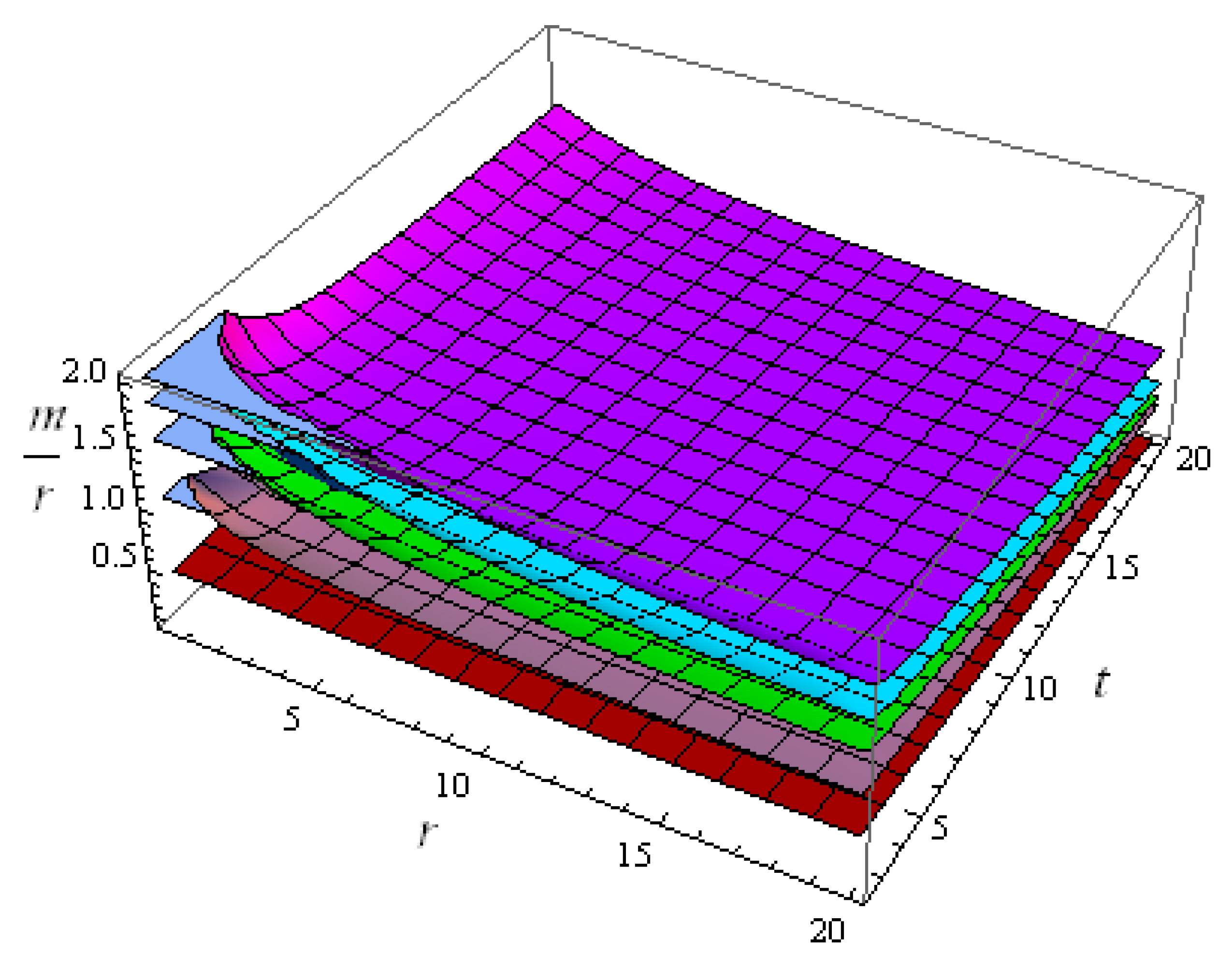
For a better understanding, we analyze this relation (26) graphically by plotting the graph of ($\frac{m}{r}$) for the model (23). Figure 1 presents the trends of ($\frac{m}{r}$) for various values of model parameter ($\alpha =0,1,3,5,7$). For all the chosen values of the parameter, ($\frac{m}{r}$) depicts maximum behavior at the core of the compact object; it gradually decreases towards the boundary with increases in r and t. However, the behavior of the graph corresponding to $\alpha =0$ (in the absence of modified terms) exhibits the existence of normal matter, as it shows less compactness in comparison to other values of $\alpha$. It enlighted the role of GB-corrections and helps us in the comparison with GB. The graphical analysis shows that a wide range of relativistic massive compact systems may arise in quadratic GB-corrections. Thus, it is expected that this effect may produce more compactness in the stellar objects than GB, which is a useful result from an observational standpoint. Consequently, we could conclude that a model of this type may help us to explore some unknown highly dense, non-static self-gravitational dissipative systems that have not been discovered in GR.

3. Differential Equation for the Weyl Curvature Scalar $\mathcal{E}$

We shall now proceed to construct a significant relation between the $\mathcal{E}$, density inhomogeneity, dissipative variables and the $f\left(\mathcal{G}\right)$ corrections. In classical GR, the Weyl tensor is used to evaluate the influence of tidal forces along with the spacetime curvature. The Weyl tensor $\left(C_{\mu \upsilon \eta }^{\sigma }\right)$ may be described in terms of certain curvature, measuring tensorial quantitative as

$$\begin{array}{c}\hfill C_{\mu \upsilon \eta }^{\sigma }=R_{\mu \upsilon \varsigma }^{\sigma }+\frac{1}{2}(R_{\mu \upsilon }{\delta }_{\eta }^{\sigma }-R_{\mu \eta }{\delta }_{\upsilon }^{\sigma }+R_{\upsilon }^{\sigma }{g}_{\mu \eta }+R_{\eta }^{\sigma }{g}_{\mu \upsilon })+\frac{1}{6}\mathbf{R}({\delta }_{\upsilon }^{\sigma }{g}_{\mu \eta }-{\delta }_{\eta }^{\sigma }{g}_{\mu \upsilon }).\end{array}$$

(28)

Generally, the quantity $C_{\mu \upsilon \eta }^{\sigma }$ can be decomposed in terms of two components: one is the magnetic component $H_{\mu \upsilon }$ (which vanishes in spherically symmetric case). However, the electric component, ($E_{\mu \upsilon }$), is defined as

$$\begin{array}{c}\hfill E_{\mu \upsilon }=C_{\mu \sigma \eta \upsilon }{V}^{\sigma }{V}^{\upsilon },\end{array}$$

(29)

whose only non-zero components are

$$\begin{array}{c}\hfill E_{11}=\frac{2\mathcal{E}}{3}{B}^2,E_{22}=-\frac{\mathcal{E}}{3}{C}^2,E_{33}=E_{22}{sin}^2\theta .\end{array}$$

Here, $\mathcal{E}$ is known as the Weyl scalar, defined as

$$\begin{array}{cc}\hfill \mathcal{E}& =-\frac{1}{2}\left[\frac{C^{″}}{C}-\frac{A^{″}}{A}-\left(\frac{C^{\prime }}{C}-\frac{A^{\prime }}{A}\right)\left(\frac{C^{\prime }}{C}+\frac{B^{\prime }}{B}\right)\right]\frac{1}{B^2}-\frac{1}{2C^2}\hfill \\ \hfill & +\frac{1}{2}\left[\frac{\ddot{C}}{C}+\left(\frac{\dot{C}}{C}+\frac{\dot{A}}{A}\right)\left(\frac{\dot{B}}{B}-\frac{\dot{C}}{C}\right)-\frac{\ddot{B}}{B}\right]\frac{1}{A^2}.\hfill \end{array}$$

(30)

The relation (29) can also be defined in an alternative form as

$$\begin{array}{c}\hfill E_{\mu \upsilon }=\mathcal{E}\left[{\chi }_{\mu }{\chi }_{\upsilon }-\frac{1}{3}{h}_{\mu \upsilon }\right].\end{array}$$

(31)

Next, using $f\left(\mathcal{G}\right)$ field equations along with Equations (20) and (30), we have

$$\begin{array}{c}\hfill \mathcal{E}=\frac{1}{2}(\rho -\mathrm{\Pi })-\frac{3m}{C^3}-\alpha \left({\psi }_1\ddot{\mathcal{G}}+{\psi }_2{\mathcal{G}}^{″}+{\psi }_3{\mathcal{G}}^{\prime }+{\psi }_4\dot{\mathcal{G}}+{\psi }_5{\dot{\mathcal{G}}}^{\prime }-{\varphi }_2{\mathcal{G}}^{″}-{\varphi }_2{\mathcal{G}}^{\prime }+{\varphi }_3\dot{\mathcal{G}}\right).\end{array}$$

(32)

Next, the integration of Equation (24) gives

$$\begin{array}{cc}\hfill m& =\frac{1}{2}{\int }_0^{\tilde{r}}\left(\rho +q\frac{U}{\tilde{E}}\right)C^2{C}^{\prime }d\tilde{r}+\alpha {\int }_0^{\tilde{r}}\left[C^2\left({\varphi }_1\ddot{\mathcal{G}}+{\varphi }_2\dot{\mathcal{G}}+{\varphi }_3{\mathcal{G}}^{\prime }\right)\right.\hfill \\ \hfill & +\left.\frac{qU}{\tilde{E}}\left({\eta }_1\dot{\mathcal{G}}+{\eta }_2{\mathcal{G}}^{\prime }+{\eta }_3{\dot{\mathcal{G}}}^{\prime }\right)\right]C^{\prime }d\tilde{r}-\frac{\alpha }{4}{\int }_0^{\tilde{r}}{\mathcal{G}}^2{C}^2{C}^{\prime }d\tilde{r}.\hfill \end{array}$$

(33)

The combination of Equations (32) and (33) implies

$$\begin{array}{cc}\hfill \mathcal{E}& =-\frac{\mathrm{\Pi }}{2}+\frac{1}{2C^3}{\int }_0^{\tilde{r}}{C}^3{\rho }^{\prime }d\tilde{r}-\frac{3}{2C^3}{\int }_0^{\tilde{r}}q\frac{U}{\tilde{E}}{C}^{\prime }{C}^{2}d\tilde{r}-\frac{3\alpha }{4}{\int }_0^{\tilde{r}}{\mathcal{G}}^2{C}^{\prime }{C}^{2}d\tilde{r}\hfill \\ \hfill & -\frac{3\alpha }{C^3}{\int }_0^{\tilde{r}}\left[C^2\left({\varphi }_1\ddot{\mathcal{G}}+{\varphi }_2\dot{\mathcal{G}}+{\varphi }_3{\mathcal{G}}^{\prime }\right)+\frac{qU}{\tilde{E}}\left({\eta }_1\dot{\mathcal{G}}+{\eta }_2{\mathcal{G}}^{\prime }+{\eta }_3{\dot{\mathcal{G}}}^{\prime }\right)\right]C^{\prime }d\tilde{r}\hfill \\ \hfill & -\alpha \left({\psi }_1\ddot{\mathcal{G}}+{\psi }_2{\mathcal{G}}^{″}+{\psi }_3{\mathcal{G}}^{\prime }+{\psi }_4\dot{\mathcal{G}}+{\psi }_5{\dot{\mathcal{G}}}^{\prime }-{\varphi }_2{\mathcal{G}}^{″}-{\varphi }_2{\mathcal{G}}^{\prime }+{\varphi }_3\dot{\mathcal{G}}\right).\hfill \end{array}$$

(34)

The above equation describes a basic relationship between the Weyl scalar, anisotropy of pressure, irregular energy density, dissipative variables and the $f\left(\mathcal{G}\right)$-contributions.

Next, we formulate an important equation for the Weyl curvature scalar that performs a primary role in this manuscript. This equation relates the Weyl scalar and some matter variables as well, as the $f\left(\mathcal{G}\right)$-corrections, to analyze the evolution of dissipative anisotropic self-gravitational fluid. This differential equation was primarily defined in [72]. Later with [73,74], from the conservation equations (Bianchi identities) can easily be obtained.

$$\begin{array}{cc}\hfill \frac{d}{dt}\left[\mathcal{E}-\frac{1}{2}(\rho -\mathrm{\Pi })\right]& =\frac{3\dot{C}}{C}\left[\frac{1}{2}(\rho +P_{\perp })-\mathcal{E}-\frac{\alpha }{A^2}\left({\varphi }_1\ddot{\mathcal{G}}+{\varphi }_2\dot{\mathcal{G}}+{\varphi }_3{\mathcal{G}}^{\prime }\right)-\frac{\alpha }{4}{\mathcal{G}}^2\right]\hfill \\ \hfill & +\frac{3}{2}\frac{A{C}^{\prime }}{BC}q+{\mathcal{X}}_1^{\left(D\right)},\hfill \end{array}$$

(35)

where the term ${\mathcal{X}}_1^{\left(D\right)}$ is defined in the appendix. This equation was originally suggested by Ellis [72,75]. Later on, it was used in several investigations regarding GR as well MGT [46,76,77]. It plays a significant function in this investigation. This is the evolution of the equation for different quantities accountable for the appearance of inhomogeneous behavior of energy–density. Against the dynamics of GR, Herrera et al. [76] discussed that the Weyl tensor, anisotropic stresses, and the dissipative variables are certain parameters for generating inhomogeneities in the framework of the self-gravitational stars. However, in our case, quadratic-$f\left(\mathcal{G}\right)$ corrections also play an effective role in controlling the inhomogeneities in the energy density distribution, alongside GR terms. The presence of higher-derivative quadratic GB corrections may increment the inhomogeneities of the energy density of the compact stars. After some manipulation, we use this differential Equation (35) as an evolution equation for the pressure anisotropy in the coming section. In this way, we may obtain certain conditions that ensure the propagation in time of anisotropy of pressure for $f\left(\mathcal{G}\right)$-corrections.

4. The Evolution of the Isotropic Pressure

The understanding of relativistic stellar systems under extreme conditions provides a crossroads of the theories regarding gravitational interactions. It represents an extensive review of the strong-field regime of standard GR and initiates productive pathways to modern cosmology and gravitational physics. This idea has given the way to different gravitational alternatives that alter the standard action of GR. These gravity models modify the TOV Equation [50] of stellar structure. This has opened a new insight to constrain the modified theories with the current and forthcoming observations of various kinds of stars. The modifications of GR involving the GB term $\left(\mathcal{G}\right)$ have recently gained a lot of attention as a possible explanation of gravitational DE.

In this respect, Abbas et al. [78] investigated the formation of anisotropic stellar structures within the dynamics of $f\left(\mathcal{G}\right)$ model of gravity. They analyzed the stability and the regularity conditions corresponding to several anisotropic compact systems. Momeni and Myrzakulov [26] formulated spherically symmetric solutions for a stellar system such as a neutron star by constructing a hydrostatic equilibrium equation (commonly known as TOV equation) in $f\left(\mathcal{G}\right)$ gravity. Momeni et al. [79] studied the dynamics of the stellar system by formulating TOV equations within the frameworks of non-local $f\left(\mathbf{R}\right)$ gravitational theory. Yousaf et al. [80] examined the effects of Palatini $f\left(\mathbf{R}\right)$ gravity on the evolution of static anisotropic compact systems by calculating the TOV equations. Momeni et al. [27] explored the modified form of the TOV equation corresponding to a static spherically symmetric stellar system in the mimetic gravity model. It is observed that the investigation of stellar systems in alternative gravity models enables us to explore some appealing astrophysical features. By assuming different realistic $f\left(\mathcal{G}\right)$ gravitational models, Shamir and Naz [29] examined several structural features of anisotropic stellar systems such as pressure anisotropy, effective density, TOV equations, mass-radius ratio as well as the stabling bounds. The same authors scrutinized the effects of the charge distribution on the isotropic compact stars by finding the TOV equations within the formalism of some realistic $f\left(\mathcal{G}\right)$ models [81]. Bhatti et al. [44,45] studied the dynamical evolution of dissipative anisotropic stellar systems with and without the influence of electric charge by formulating the corresponding complexity factor.

We proceed by taking into consideration the role of radial and tangential pressure in the concept of “asymmetry”, through the mechanism of classical GR. The TOV equation for the an anisotropic stellar system as defined in Equation (25) is

$$\begin{array}{cc}\hfill P_r^{\prime }& =-\left[\rho +P_r-\frac{1}{B^4}\left({\phi }_1{\mathcal{G}}^{″}+{\phi }_2{\mathcal{G}}^{\prime }+{\phi }_3\dot{\mathcal{G}}\right)+\frac{2\alpha }{A^2{B}^2}\left({\varphi }_1\ddot{\mathcal{G}}+{\varphi }_2\dot{\mathcal{G}}\right.\right.\hfill \\ \hfill & \left.\left.+{\varphi }_3{\mathcal{G}}^{\prime }\right)\right]\frac{A^{\prime }}{A}+\left[2(P_{\perp }-P_r)-\frac{2}{B^4}\left\{\left({\phi }_1{\mathcal{G}}^{″}+{\phi }_2{\mathcal{G}}^{\prime }+{\phi }_3\dot{\mathcal{G}}\right)\right\}2\alpha \right]\frac{C^{\prime }}{C}\hfill \\ \hfill & +\frac{\alpha }{2B^2}{\mathcal{GG}}^{\prime }+{\mathcal{T}}^{\left(\mathcal{G}\right)}.\hfill \end{array}$$

(36)

The above-stated expression is also known as the hydrostatic equilibrium equation in which every term has a well-known physical meanings. Here, $P_r^{\prime }$ simply represents the gradient of pressure opposing the gravity, the second and the third term correspond to the gravitational force and the influence of pressure anisotropy, while the remaining terms signify the $f\left(\mathcal{G}\right)$-corrections. It is important to note that $P_r$ combines with the gravitational force term, while $P_{\perp }$ fails to do so. This fact describes why the compactness of anisotropic spherical sources is greater than those of isotropic ones, if $P_r<P_{\perp }$. In Newtonian hydrodynamics, $P_r=0$, in the second term of Equation (35), represents an intrinsic anisotropy. Now, we propose the following explanation regarding the origin of the degression of the anisotropic pressure condition during the evolution of a gravitational structure, departing the equilibrium state from a static matter configuration having isotropic pressure. For this, we consider that the gravitational source is constrained to leave its equilibrium state. Following that, we assume a picture of the system just after the abandoning, at a time scale smaller than the hydrostatic time, thermal adjustment time and the thermal relaxation time. Thus, at such a time scale, we get

$$\begin{array}{c}\hfill q\approx U\approx \mathrm{\Theta }\approx \sigma \approx 0\Rightarrow \dot{C}\approx \dot{B}\approx 0,\end{array}$$

(37)

where it is notable that the t-derivative of the above-stated quantities is very small but non-zero. Next, using the $f\left(\mathcal{G}\right)$ gravitational equations along with the assumption that the considered fluid is initially isotropic we evaluate the anisotropic pressure scalar $\mathrm{\Pi }$ as

$$\begin{array}{cc}\hfill \mathrm{\Pi }+& \left[\frac{2\alpha }{B^2}\left({\phi }_1{\mathcal{G}}^{″}+{\phi }_2{\mathcal{G}}^{\prime }+{\phi }_3\dot{\mathcal{G}}\right)-\frac{1}{C^2}\left({\psi }_1\ddot{\mathcal{G}}+{\psi }_2{\mathcal{G}}^{″}+{\psi }_3{\mathcal{G}}^{\prime }+{\psi }_4\dot{\mathcal{G}}+{\psi }_5{\dot{\mathcal{G}}}^{\prime }\right)\right]\hfill \\ \hfill & \approx \frac{1}{A}\left(\frac{\ddot{B}}{B}-\frac{\ddot{C}}{C}\right)\approx \dot{\sigma }.\hfill \end{array}$$

(38)

Consequently, we deduce that under the considered time scale, the system will leave the original isotropic pressure condition unless we consider the shear-free ($\sigma =0$) evolution of the fluid. It is notable that as the gravitational system leaves its equilibrium state, two possible situations arise:

• The dissipative fluid distribution is stable within the considered time scale (hydrostatic time);
• The fluid distribution turns unstable and enters into the time-dependent regime, unless it reaches the final state of equilibrium.

In the first scenario, the pressure anisotropy described by Equation (38) should not vanish in the new state of equilibrium. Thus, the consequent distribution, despite being static, represents the anisotropy of pressure, contrary to the first one. However, in the second scenario, the degression from the pressure isotropy condition is compulsory, despite the shear-free evolution, for any scale of time. Then, utilizing Equations (A16) and (35), we have

$$\begin{array}{cc}\hfill & \frac{d}{dt}\left(\mathcal{E}+\frac{\mathrm{\Pi }}{2}\right)+\frac{\dot{C}}{C}\left(3\mathcal{E}+\frac{\mathrm{\Pi }}{2}\right)-\frac{\alpha }{2A}\mathcal{G}\dot{\mathcal{G}}-\frac{A}{2}{\mathcal{Y}}_1^{\left(\mathrm{D}\right)}\hfill \\ \hfill & =-\frac{\sigma }{2}(\rho +P_r)A-\frac{A}{2B}q-3\alpha \frac{\dot{C}}{C}\left[\frac{1}{4}{\mathcal{G}}^2-\frac{1}{A^2}\left({\varphi }_1\ddot{\mathcal{G}}+{\varphi }_2\dot{\mathcal{G}}+{\varphi }_3{\mathcal{G}}^{\prime }\right)\right]\hfill \\ \hfill & -\frac{1}{2B}\left(2A^{\prime }-\frac{A{C}^{\prime }}{C}\right)+\frac{A}{4A^{\prime }}\alpha \mathcal{G}+{\mathcal{X}}_1^{\left(\mathrm{D}\right)}.\hfill \end{array}$$

(39)

The above equation corresponds to Equation (24) of [46] for GR, with the difference that it also includes the extra-curvature $f\left(\mathcal{G}\right)$-corrections. Next, considering the dissipative constituent ${\mathrm{\Phi }}_{\mathrm{diss}}$ as

$$\begin{array}{c}\hfill {\mathrm{\Phi }}_{\mathrm{diss}}\equiv -\frac{1}{2B}\left[q^{\prime }A+\left(2A^{\prime }-\frac{A{C}^{\prime }}{C}\right)q\right].\end{array}$$

(40)

Therefore, Equation (39) reads

$$\begin{array}{cc}\hfill & \dot{\mathrm{\Pi }}+\mathrm{\Pi }\frac{\dot{C}}{C}+2\left(\dot{\mathcal{E}}+3\mathcal{E}\frac{\dot{C}}{C}\right)-\frac{\alpha }{A}\mathcal{G}\dot{\mathcal{G}}-A{\mathcal{Y}}_1^{\left(D\right)}\hfill \\ \hfill & =-\sigma (\rho +P_r)A+2{\mathrm{\Phi }}_{\mathrm{diss}}-3\alpha \frac{\dot{C}}{C}\left[\frac{1}{4}{\mathcal{G}}^2-\frac{1}{A^2}\left({\varphi }_1\ddot{\mathcal{G}}+{\varphi }_2\dot{\mathcal{G}}+{\varphi }_3{\mathcal{G}}^{\prime }\right)\right]\hfill \\ \hfill & +\frac{A}{2A^{\prime }}\alpha \mathcal{G}+2{\mathcal{X}}_1^{\left(\mathrm{D}\right)},\hfill \end{array}$$

(41)

which is an evolution equation for the anisotropic factor $\mathrm{\Pi }$. Observe that the above-stated expression also corresponds to the Equation (26) of [46] for GR, with a difference of higher-order terms emerging due to $f\left(\mathcal{G}\right)$ gravity. Then, integrating the last equation under the initial condition ($\mathrm{\Pi }=0$ at $t=0$), we get

$$\begin{array}{cc}\hfill \mathrm{\Pi }& =-\frac{2}{C}{\int }_0^{\tilde{r}}\left(\dot{\mathcal{E}}+3\mathcal{E}\frac{\dot{C}}{C}\right)Cd\tilde{t}-\frac{1}{C}{\int }_0^{\tilde{r}}\sigma (\rho +P_r)ACd\tilde{t}+\frac{2}{C}{\int }_0^{\tilde{r}}{\mathrm{\Phi }}_{\mathrm{diss}}Cd\tilde{t}\hfill \\ \hfill & +\frac{\alpha }{C}\left({\int }_0^{\tilde{r}}\frac{C}{A}\mathcal{G}\dot{\mathcal{G}}\right)d\tilde{t}+\frac{1}{C}{\int }_0^{\tilde{r}}CA{\mathcal{Y}}_1^{\left(D\right)}d\tilde{t}+\frac{2}{C}{\int }_0^{\tilde{r}}C{\mathcal{X}}_1^{\left(\mathrm{D}\right)}d\tilde{t}\hfill \\ \hfill & -\frac{3\alpha }{C}{\int }_0^{\tilde{r}}C\frac{\dot{C}}{C}\left[\frac{1}{4}{\mathcal{G}}^2-\frac{1}{A^2}\left({\varphi }_1\ddot{\mathcal{G}}+{\varphi }_2\dot{\mathcal{G}}+{\varphi }_3{\mathcal{G}}^{\prime }\right)\right]d\tilde{r}.\hfill \end{array}$$

(42)

Here, it is worth-mentioning that there are three factors plus the $f\left(\mathcal{G}\right)$ contributions causing the self-gravitational fluid to leave the isotropic pressure condition. In this equation, the first integral describes the contribution of the Weyl tensor, the second integral corresponds to the shear stress of the fluid distribution, the third one explains the influence of dissipative phenomenons using ${\mathrm{\Phi }}_{\mathrm{diss}}$, and the remaining factors show the contribution of $f\left(\mathcal{G}\right)$ dark source terms that also affect pressure isotropy. Now, we reformulate the above equation by representing the Weyl tensor termss with the help of Equation (34).

$$\begin{array}{cc}\hfill \mathrm{\Pi }\dot{C}& =\frac{C}{2}(\rho +P_r)A\sigma -{\mathrm{\Phi }}_{\mathrm{diss}}C+\frac{3\alpha }{2}\left[\frac{1}{4}{\mathcal{G}}^2-\frac{1}{A^2}\left({\varphi }_1\ddot{\mathcal{G}}+{\varphi }_2\dot{\mathcal{G}}+{\varphi }_3{\mathcal{G}}^{\prime }\right)\right]C\hfill \\ \hfill & -C{\mathcal{X}}_1^{\left(\mathrm{D}\right)}+\frac{1}{2C^2}\frac{d}{dt}\left({\int }_0^{\tilde{r}}{\rho }^{\prime }{C}^{3}d\tilde{r}\right)-\frac{3\alpha }{4C^2}\left(\frac{d}{dt}{\int }_0^{\tilde{r}}{\mathcal{G}}^2{C}^2{C}^{\prime }d\tilde{r}\right)\hfill \\ \hfill & +\frac{3\alpha }{C^2}\left(\frac{d}{dt}{\int }_0^{\tilde{r}}\frac{C^2}{A^2}\left({\varphi }_1\ddot{\mathcal{G}}+{\varphi }_2\dot{\mathcal{G}}+{\varphi }_3{\mathcal{G}}^{\prime }\right)C^{\prime }d\tilde{r}\right)-\frac{3}{2C^2}\left({\int }_0^{\tilde{r}}q\frac{U}{\tilde{E}}{C}^{\prime }{C}^{2}d\tilde{r}\right)\hfill \\ \hfill & +\frac{3\alpha }{C^2}\left(\frac{d}{dt}{\int }_0^{\tilde{r}}\frac{U}{\tilde{E}}\frac{C^2}{A^2}({\eta }_1\dot{\mathcal{G}}+{\eta }_2{\mathcal{G}}^{\prime }+{\eta }_3{\dot{\mathcal{G}}}^{\prime })d\tilde{r}\right).\hfill \end{array}$$

(43)

From the above-mentioned equation, we may deduce that the self-gravitational structure will leave the isotropic pressure condition only in a case where all the terms on the right-hand side cancel each other. This is unlike in the case of GR (Equation (28) of [46]), where the isotropy condition depends on the first four factors only. Here, the $f\left(\mathcal{G}\right)$-corrections also contribute to the anisotropy factor and force the system to abandon the pressure isotropy condition. Therefore, it appears that the presence of higher-curvature stringy corrections is forcing the system to leave the initially isotropic fluid configuration. Thus, the modification of gravity increases the anisotropy, unless we assume a highly unlikely cancelation of all the terms on the right side occurs.

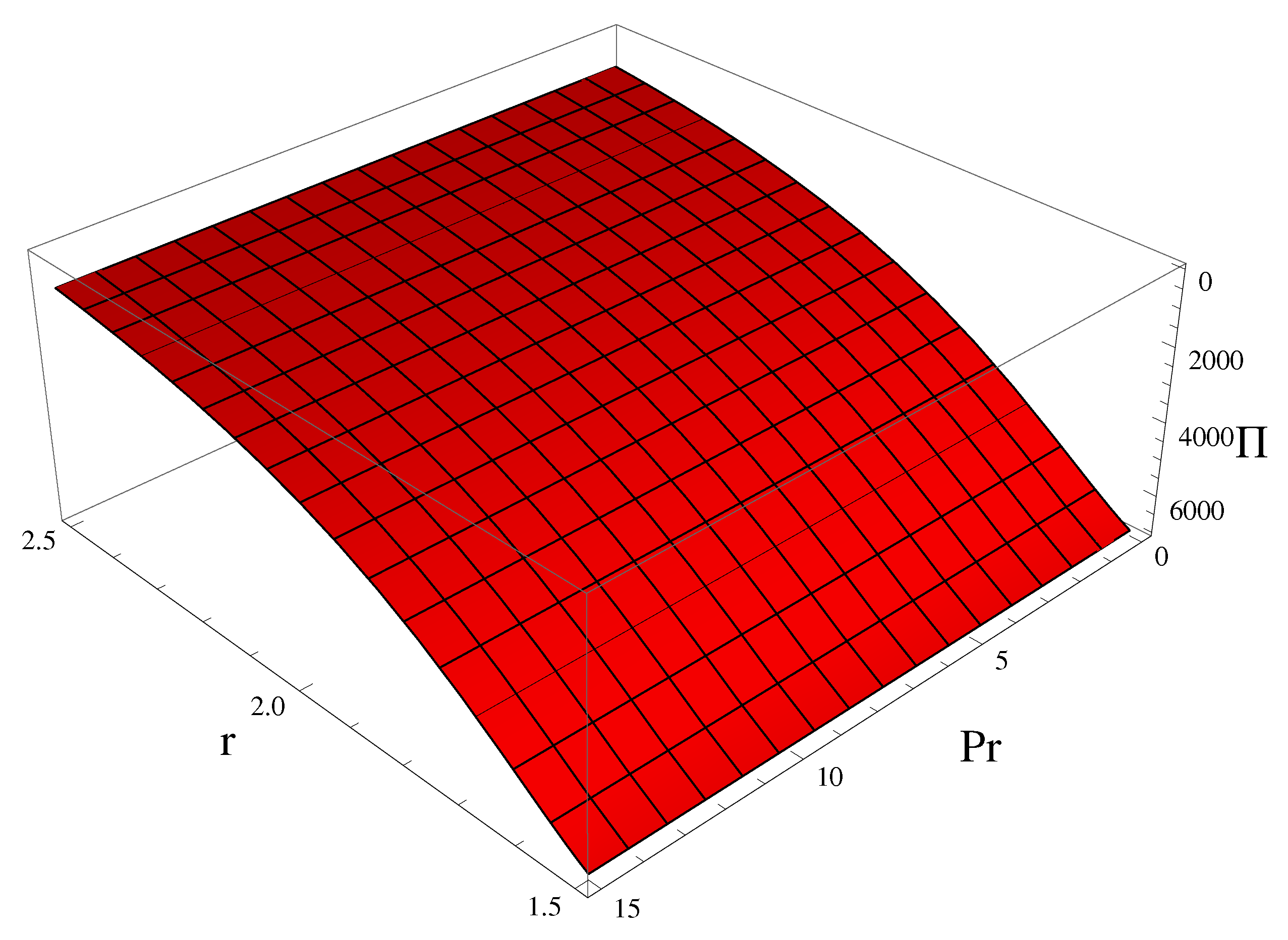
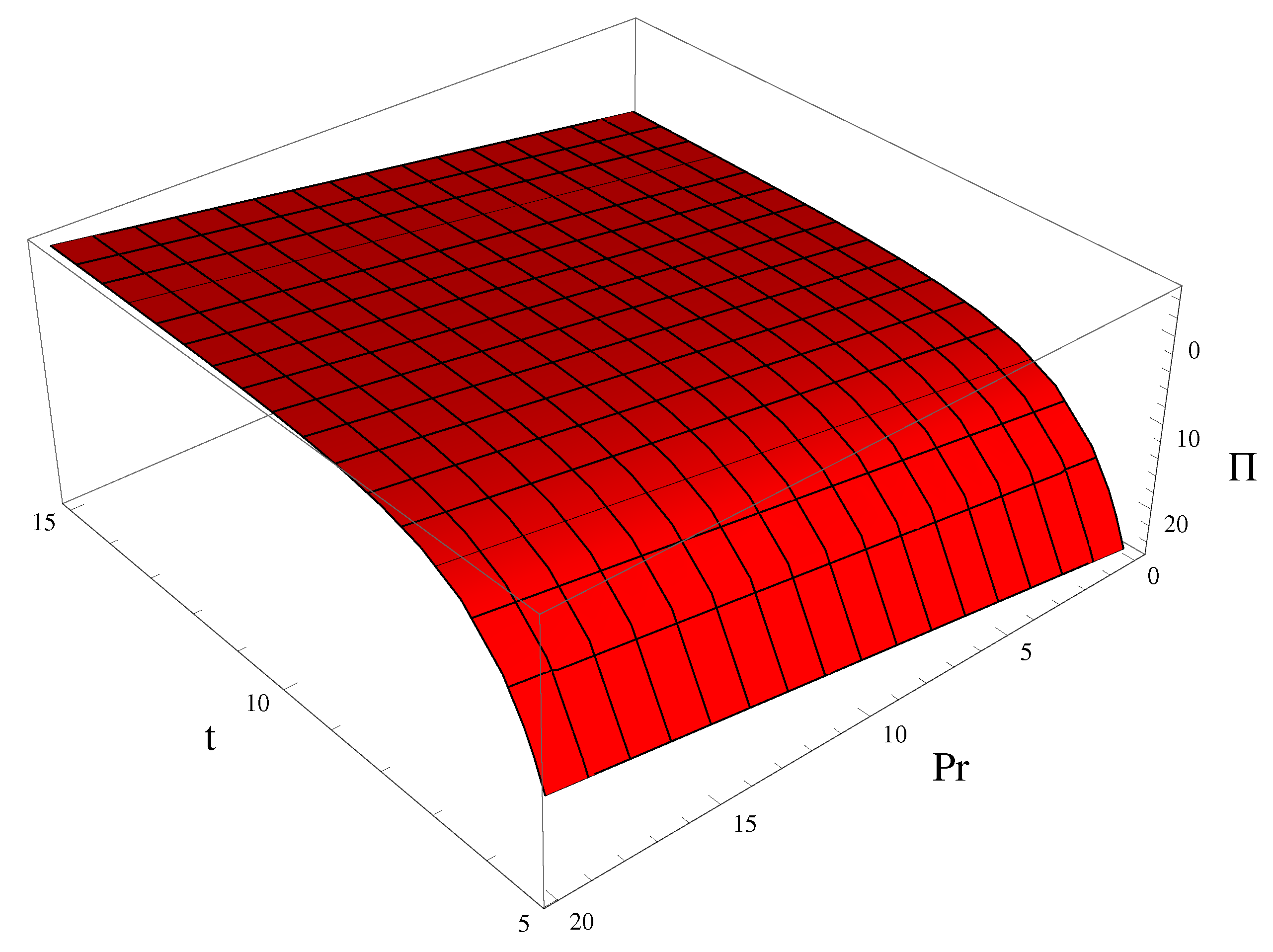
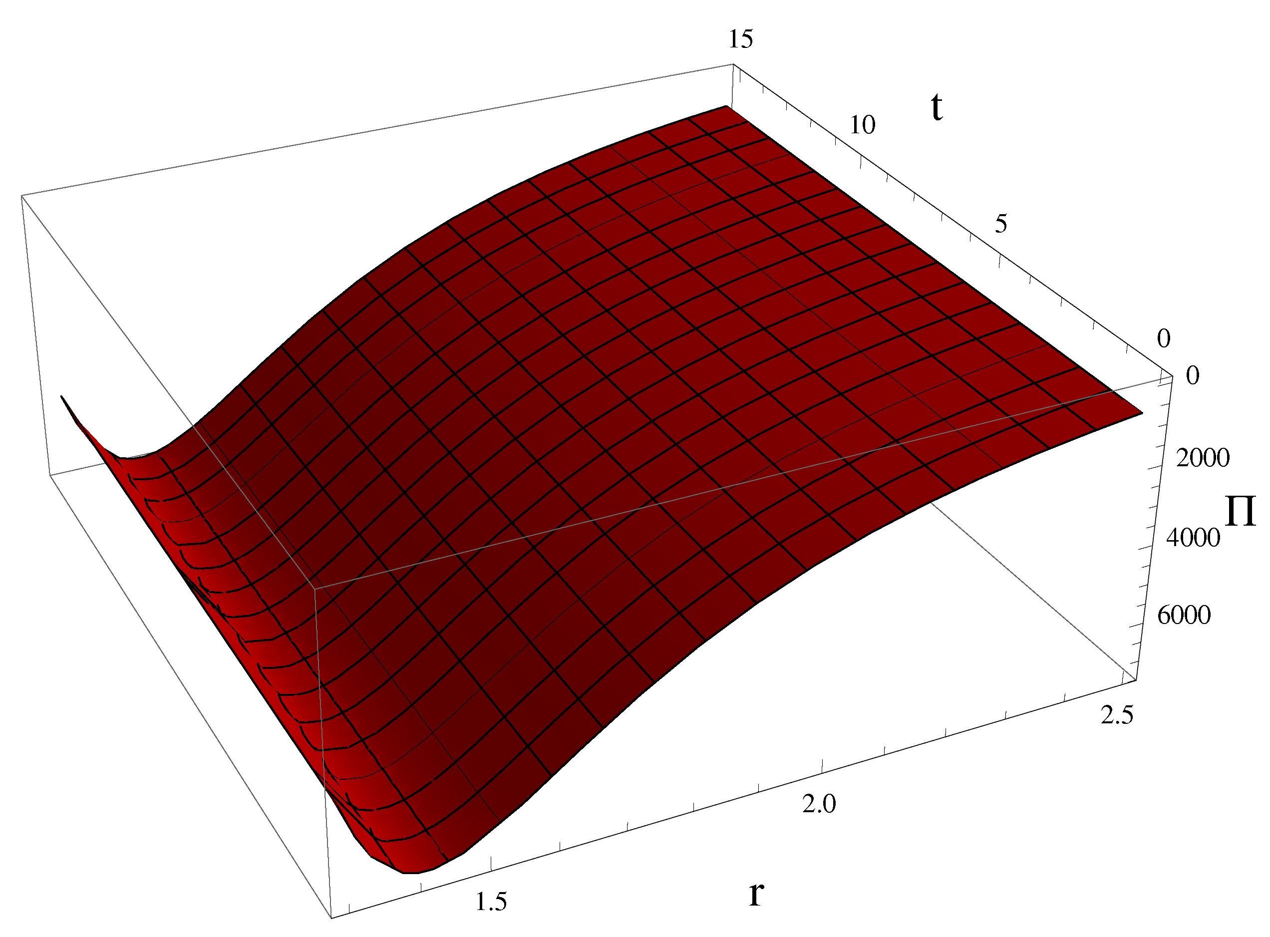
We have presented the effects of the various components of Equations (41) and (42) using graphical analysis by considering the Krori and Barua ansatz [71] presented in Equation (26). We analyze the contributions of different fluid components and the higher-curvature terms graphically. The graphical analysis showed how an initially isotropic matter configuration becomes anisotropic due to the presence of dissipative fluxes, shear, density inhomogeneity and higher-curvature terms emerging from GB-gravity. The graphical analysis (described in Figure 2, Figure 3 and Figure 4) shows that the anisotropy is minimal at the center and is maximal at the boundary. In this respect, Maurya et al. [82] suggested the generalized anisotropic stellar models of embedding class one by describing their physical characteristics. In addition, Maurya et al. [83] discussed the existence of anisotropic compact objects for $f(\mathcal{G},T)$ gravity. Mustafa et al. [84] explored the physical features of the anisotropic compact systems through modified teleparallel gravity. Our analysis shows that the presented results are compatible with the above-mentioned studies.

5. Conclusions

During the last few decades, some primary findings have been realized with respect to relativistic, as well as Newtonian fluids, by taking into account the isotropic pressure condition. On the other hand, it is well established that the existence of a small number of anisotropies in the fluid’s pressure may cause different consequences under the same general condition. We also know that several physical phenomena that cause pressure anisotropy are likely to exist in very gravitational compact systems. From the above discussion, there stems an important question: under which situation does an initially isotropic fluid distribution remain isotropic throughout the evolution of the compact system? A detailed investigation is provided at the start of Section 5 for a spherically symmetric fluid configuration, which justifies the tendency of a gravitational structure to leave the pressure isotropy condition. In addition, this outcome implies that if a stable matter configuration returns to a new equilibrium state, after being eliminated from this condition, the configuration would turn out to be anisotropic.

Afterward, we analyzed the physical factors producing pressure anisotropy in the spherically symmetric fluid distribution in detail. From Equation (43), it can be easily identified that these physical factors are heat dissipation represented by the dissipative factor ${\mathrm{\Phi }}_{\mathrm{diss}}$, shear, inhomogeneous energy density and the $f\left(\mathcal{G}\right)$-corrections. Thus, we conclude that an initially isotropic (in pressure) fluid distribution will remain in this condition throughout its evolution, only if the fluid is homogeneous (in energy density), shear-free ($\sigma =0$), non-dissipative ($q=0$) and the higher-curvature $f\left(\mathcal{G}\right)$-corrections vanish; this must occur unless all the terms on the right-hand side of Equation (43) vanish. In addition, Equation (42) shows that the stability of isotropic pressure can be ensured from certain conditions including the nonexistence of dissipation, disappearance of the shear, conformal flatness and the vanishing of the $f\left(\mathcal{G}\right)$ terms; this is again shown by omitting the possibility of cancellation of all these factors.

Herrera [46] studied several sources causing inhomogeneities in the distribution of energy density. He also examined the evolution of these sources from originally homogeneous configuration for self-gravitational fluids, through the mechanism of GR. He reported that a particular combination of pressure anisotropy, dissipative variables, and shear generates inhomogeneities in energy density. In [85], it is also identified that a single dynamical variable (scalar function) originating from the orthogonal splitting of the curvature tensor controls the departure of the anisotropic fluids from the shear-free condition. This dynamical variable entails a specific combination of inhomogeneous density, dissipative variables and pressure anisotropy. Here, it is notable that, in our case, this function also incorporates the higher-order $f\left(\mathcal{G}\right)$-corrections. Therefore, even if we make the assumption of vanishing of the inhomogeneous energy density, shearing stress as well as the pressure anisotropy, in this case, the dissipative variables will increase the digression of the pressure isotropy condition in two ways:

• By considering its contribution as characterized by Equation (43).
• By incorporating the degression of the homogeneous energy density and the absence of shear ($\sigma =0$).

Consequently, we can deduce that the fluid distribution evolves by possessing the pressure isotropy condition throughout its evolution, only under the conditions of non-dissipation, shear-free, conformal flatness and the non-existence of GB corrections.

The central theme of this investigation is to explore the influence of the quadratic-GB gravitational model on the modeling of non-static anisotropic self-gravitational compact stars that would be interesting to study further in the future. We have examined the physical aspects of the non-static stellar structure through mass-radius relationships. The behavior of compactness of the anisotropic compact system corresponding to r and t for different values of model parameter offer interesting future directions for this work. More concisely, the considered realistic form of the $f\left(\mathcal{G}\right)$-gravity model thoroughly justifies the role of the GB-correction on the anisotropies of the spherically symmetric self-gravitational fluids, as well as the stability of pressure anisotropy of the system. In addition, it is worth mentioning that the presence of higher-curvature GB corrections follows physically accepted phenomena and the resulting outcomes are consistent with the experimental data. This shows the viability of the assumed gravity model in the realm of $f\left(\mathcal{G}\right)$-theory.