An Inertial Subgradient Extragradient Method for Approximating Solutions to Equilibrium Problems in Hadamard Manifolds

Abstract

In this work, we are concerned with the iterative approximation of solutions to equilibrium problems in the framework of Hadamard manifolds. We introduce a subgradient extragradient type method with a self-adaptive step size. The use of a step size which is allowed to increase per iteration is to avoid the dependence of our method on the Lipschitz constant of the underlying operator as has been the case in recent articles in this direction. In general, operators satisfying weak monotonicity conditions seem to be more applicable in practice. By using inertial and viscosity techniques, we establish a convergence result for solving a pseudomonotone equilibrium problem under some appropriate conditions. As applications, we use our method to solve some theoretical optimization problems. Finally, we present some numerical illustrations in order to demonstrate the quantitative efficacy and superiority of our proposed method over a previous method present in the literature.

1. Introduction

The minimax inequality introduced in 1972 by Ky Fan [1], later renamed as Equilibrium Problem (EP), plays a major role in many fields and provides a unified framework for the study of variational inequalities, game theory, mathematical economics, fixed point theory and optimization theory. The use of the term equilibrium problem is credited to the 1994 paper by Blum and Oetlli [2], which followed an earlier article by Muu and Oetlli [3]. In the latter paper, three standard examples of the EP were given, viz: fixed point, convex minimization and variational inequality problems. The EP also includes as examples, convex differentiable optimization, complementarity, saddle point and Nash equilibrium problem [2,3]. Let $g:K\times K\to \mathbb{R}$ be a bifunction such that $g(x,x)=0$ for all $x\in K$, where K is a nonempty subset of a topological space X. Then, the EP calls for finding a point $x\in K$ such that

$$g(x,y)\ge 0\forall y\in K.$$

The study of variational inequality, equilibrium and other related optimization problems has recently received considerable attention from researchers in the framework of Riemannian manifolds. Thus, methods and ideas have been extended from linear settings to this more general setting. These generalizations become necessary because of the advantages they bring forth. For example, nonconvex optimization problems can easily be transformed into problems of convex type by choosing a suitable Riemannian metric [4,5,6]. Another advantage of this extension is that constrained optimization problems can be viewed as unconstrained ones [4,6,7,8]. As a result, classical methods for solving optimization problems have been extended from linear frameworks to Riemannian manifolds. In 2012, Colao et al. [9] studied equilibrium problems on Hadamard manifolds in the following setting: Let K be a nonempty, closed and convex subset of an Hadamard manifold M and let $g:K\times K\to \mathbb{R}$ be a bifunction satisfying $g(x,x)=0$ for all $x\in M$. An equilibrium problem (EP, for short) on a manifold consists of finding

$$\begin{array}{c}\hfill x\in K\mathrm{such}\mathrm{that}g(x,y)\ge 0\forall y\in K.\end{array}$$

(1)

We denote by $Sol(g,K)$ the solution set of the EP (1). By developing and proving Fan’s KKM Lemma, Colao et al. [9] studied the existence of solutions to the EP in the framework of Hadamard spaces. For many other studies and results in this direction, see, for example, [10,11,12].

The development of an effective iterative algorithm for approximating solutions to optimization problems is another interesting area of research in nonlinear analysis and optimization theory. Iterative approximation of solutions to equilibrium problems in any setting, whether linear or nonlinear, includes, for example, the use of the Extragradient Method (EGM) proposed by Korpelevich [13]. The EGM was initially used for solving saddle point problems. It was later adapted for solving variational inequality and then equilibrium problems. Inspired by the EGM and the perceived drawbacks of the method, Censor et al. [14] introduced the Subgradient Extragradient Method (SEGM), which has since been used for solving both variational and equilibrium problems. For solving EPs, Tran et al. [15] introduced an extragradient-like method for approximating solutions to pseudomonotone equilibrium problems. Using an alternative approach, Nguyen et al. [16] introduced a method for finding common solutions to fixed point and equilibrium problems, which is based on the extragradient method proposed in [15]. More recently, Rehman et al. [17] introduced an inertial subgradient extragradient algorithm for solving equilibrium problems. Using a viscosity approach, they proved a strong convergence theorem for an algorithm approximating solutions to EPs with pseudomonotone bifunctions. For more contributions regarding methods for solving EPs in linear settings, see, for example, [12,18,19,20,21].

We note that several of the methods discussed above have been extended to EPs on Hadamard manifolds. The first work of Colao et al. [9] was followed by those of Salahuddin [10] and Li et al. [21]. Neto et al. [22] extended the result of Nguyen et al. [16] to this setting by considering the following algorithm: Given ${\lambda }_n>0$, compute

$$\begin{array}{c}\hfill \left\{\begin{array}{c}{y}_n=arg\underset{z\in M}{min}\{g(x_n,z)+\frac{1}{2{\lambda }_n}{d}^2(x_n,z),\hfill \\ x_{n+1}=arg\underset{z\in M}{min}\{g(y_n,z)+\frac{1}{2{\lambda }_n}{d}^2(x_n,z),\hfill \end{array}\right.\end{array}$$

where $0\le {\lambda }_n<\mu <min\{\frac{1}{c_1},\frac{1}{c_2}\}$, and $c_1>0$ and $c_2>0$ are the Lipschitz constants of the bifunction g. Fan et al. [23] proposed an explicit extragradient method for solving pseudomonotone equilibrium problems on Hadamard manifolds. Their method uses a variable step size which is monotonically decreasing. These authors proved a convergence theorem for their method and also established an R-linear convergence result for the proposed method. Very recently, Ali-Akbari [24] has introduced a subgradient extragradient algorithm for approximating solutions to EPs on Hadamard manifolds and has proved a convergence theorem for approximating solutions to pseudomonotone equilibrium problems. This theorem depends on the Lipschitz constants of the corresponding bifunctions.

The inertial technique finds crucial application in the construction of effective and accelerated algorithms in fixed point and optimization theory (see, for instance, [25,26]). In this method, the next iterate is determined by two preceding iterates ($x_{n-1}$ and $x_n$) and an inertial parameter ${\theta }_n$ which controls the momentum $x_n-x_{n-1}$. For more recent developments regarding inertial algorithms, we refer the readers to [25,27,28] and to references therein. At this point, we recall that the viscosity method due to Moudafi [29] for a nonexpansive mapping S and a given strict contraction f over K is given by $x_0\in K$ and $x_{n+1}={\beta }_{n}f\left(x_n\right)+(1-{\beta }_n)S{x}_n,n\ge 0$, where the sequence $\left\{{\beta }_n\right\}\subset (0,1)$ converges to zero. The viscosity method has also been adapted to the framework of Hadamard manifolds (see [30,31]). In this setting, the sequence $\left\{x_n\right\}$ starting with an arbitrary point $x_0\in K$ is given by

$$x_{n+1}={exp}_{f\left(x_n\right)}(1-{\beta }_n){exp}_{f\left(x_n\right)}^{-1}S{x}_n\forall n\ge 0.$$

Motivated by the subgradient method of [14], the viscosity approach [30,31,32], and by Rehman et al. [17,27] and Ali-Akbari [24], we introduce an inertial subgradient extragradient algorithm for approximating solutions to equilibrium problems on Hadamard manifolds. Employing the viscosity technique, we propose an algorithm for approximating solutions to pseudomonotone equilibrium problems and establish a convergence theorem for it. The proposed algorithm uses a self-adaptive step length which is allowed to increase during the execution of the method. In this way, dependence of the method on the Lipschitz constants is dispensed with. In order to be more precise, we now highlight the following advantages of our result over previous results announced in this direction in the literature:

(i)

The method in the present paper uses an adaptive step size which is allowed to increase from iteration to iteration unlike the method in [23,33], where the step sizes decrease monotonically, and the method of [17,24,27], which relies on the Lipschitz condition imposed on the bifunction. Since the relevant Lipschitz constants can be difficult to estimate, this affects the efficiency of the method;

(ii)

We note that the sequence of control parameters of the viscosity step of our method is only required to be non-summable. This differs from [30,32], where an extra condition (that the difference between successive parameters be summable) is imposed;

(iii)

The use of the inertial technique makes the convergence of our algorithm faster than that of the method used in [23,24];

(iv)

Our result is obtained in the framework of an Hadamard manifold unlike the results of [15,16,17], which were obtained in real Hilbert spaces.

The rest of our paper is organized as follows: First, we recall some useful definitions and preliminary results in Section 2. In Section 3, we introduce our proposed method, state our main result and present its convergence analysis. Two applications are presented in Section 4. In Section 5, we present the results of a numerical experiment which shows the efficiency of our method. We provide some concluding remarks in Section 6.

2. Preliminaries

Let M be an m-dimensional manifold, let $x\in M$ and let $T_{x}M$ be the tangent space of M at $x\in M$. We denote by $TM={\bigcup }_{x\in M}{T}_{x}M$ the tangent bundle of M. An inner product $\mathcal{R}\langle ·,·\rangle$ is called a Riemannian metric on M if ${\langle ·,·\rangle }_x:T_{x}M\times T_{x}M\to \mathbb{R}$ is an inner product for all $x\in M.$ The corresponding norm induced by the inner product ${\mathcal{R}}_x\langle ·,·\rangle$ on $T_{x}M$ is denoted by ${\parallel ·\parallel }_x.$ We will drop the subscript x and adopt $\parallel ·\parallel$ for the corresponding norm induced by the inner product. A differentiable manifold M endowed with a Riemannian metric $\mathcal{R}\langle ·,·\rangle$ is called a Riemannian manifold. In what follows, we denote the Riemannian metric $\mathcal{R}\langle ·,·\rangle$ by $\langle ·,·\rangle$ when no confusion arises. Given a piecewise smooth curve $\gamma :[a_1,a_2]\to M$ joining x to y (that is, $\gamma \left(a_1\right)=x$ and $\gamma \left(a_2\right)=y$), we define the length $l\left(\gamma \right)$ of $\gamma$ by $l\left(\gamma \right):={\int }_{a_1}^{a_2}\parallel {\gamma }^{\prime }\left(t\right)\parallel dt$. The Riemannian distance $d(x,y)$ is the minimal length over the set of all such curves joining x to y. The metric topology induced by d coincides with the original topology on M. We denote by ∇ the Levi–Civita connection associated with the Riemannian metric [34].

Let $\gamma$ be a smooth curve in M. A vector field X along $\gamma$ is said to be parallel if ${\nabla }_{{\gamma }^{\prime }}X=\mathbf{0}$, where $\mathbf{0}$ is the zero tangent vector. If ${\gamma }^{\prime }$ itself is parallel along $\gamma$, then we say that $\gamma$ is a geodesic and $\parallel {\gamma }^{\prime }\parallel$ is a constant. If  $\parallel {\gamma }^{\prime }\parallel =1$, then the geodesic $\gamma$ is said to be normalized. A geodesic joining x to y in M is called a minimizing geodesic if its length equals $d(x,y)$. A Riemannian manifold M equipped with a Riemannian distance d is a metric space $(M,d)$. A Riemannian manifold M is said to be complete if for all $x\in M$, all geodesics emanating from x are defined for all $t\in \mathbb{R}$. The Hopf–Rinow theorem [34] posits that if M is complete, then any pair of points in M can be joined by a minimizing geodesic. Moreover, if $(M,d)$ is a complete metric space, then every bounded and closed subset of M is compact. If M is a complete Riemannian manifold, then the exponential map ${exp}_x:T_{x}M\to M$ at $x\in M$ is defined by

$${exp}_{x}v:={\gamma }_v(1,x)\forall v\in T_{x}M,$$

where ${\gamma }_v(·,x)$ is the geodesic starting from x with velocity v (that is, ${\gamma }_v(0,x)=x$ and ${\gamma }_v^{\prime }(0,x)=v$). Then, for any $t,$ we have ${exp}_{x}tv={\gamma }_v(t,x)$ and ${exp}_x\mathbf{0}={\gamma }_v(0,x)=x.$ Note that the mapping ${exp}_x$ is differentiable on $T_{x}M$ for every $x\in M.$ The exponential map ${exp}_x$ has an inverse ${exp}_x^{-1}:M\to T_{x}M.$ For any $x,y\in M,$ we have $d(x,y)=\parallel {exp}_y^{-1}x\parallel =\parallel {exp}_x^{-1}y\parallel$ (see [34] for more details). The parallel transport $P_{\gamma ,\gamma \left(a_2\right),\gamma \left(a_1\right)}:T_{\gamma \left(a_1\right)}M\to T_{\gamma \left(a_2\right)}M$ on the tangent bundle $TM$ along $\gamma :[a_1,a_2]\to \mathbb{R}$ with respect to ∇ is defined by

$$P_{\gamma ,\gamma \left(a_2\right),\gamma \left(a_1\right)}v=F\left(\gamma \left(a_2\right)\right),\forall a_1,a_2\in \mathbb{R}\mathrm{and}v\in T_{\gamma \left(a_1\right)}M,$$

where F is the unique vector field such that ${\nabla }_{{\gamma }^{\prime }\left(t\right)}F=\mathbf{0}$ for all $t\in [a_1,a_2]$ and $F\left(\gamma \left(a_1\right)\right)=v.$ If $\gamma$ is a minimizing geodesic joining x to $y,$ then we write $P_{y,x}$ instead of $P_{\gamma ,y,x}.$ Note that for every $a_1,a_2,r,s\in \mathbb{R},$ we have

$$P_{\gamma \left(s\right),\gamma \left(r\right)}\circ P_{\gamma \left(r\right),\gamma \left(a_1\right)}=P_{\gamma \left(s\right),\gamma \left(a_1\right)}\mathrm{and}{P}_{\gamma \left(a_2\right),\gamma \left(a_1\right)}^{-1}=P_{\gamma \left(a_1\right),\gamma \left(a_2\right)}.$$

Additionally, $P_{\gamma \left(a_2\right),\gamma \left(a_1\right)}$ is an isometry from $T_{\gamma \left(a_1\right)}M$ to $T_{\gamma \left(a_2\right)}M,$ that is, the parallel transport preserves the inner product

$$\begin{array}{c}\hfill {\langle P_{\gamma \left(a_2\right),\gamma \left(a_1\right)}\left(u\right),P_{\gamma \left(a_2\right),\gamma \left(a_1\right)}\left(v\right)\rangle }_{\gamma \left(a_2\right)}={\langle u,v\rangle }_{\gamma \left(a_1\right)},\forall u,v\in T_{\gamma \left(a_1\right)}M.\end{array}$$

(2)

We now give some examples of Hadamard manifolds.

• Space 1: Let ${\mathbb{R}}_{++}=\{x\in \mathbb{R}:x>0\}$ and $M=({\mathbb{R}}_{++},\langle ·,·\rangle )$ be the Riemannian manifold equipped with the inner product $\langle x,y\rangle =xy\forall x,y\in \mathbb{R}.$ Since the sectional curvature of M is zero [35], M is an Hadamard manifold. Let $x,y\in M$ and $v\in T_{x}M$ with ${\parallel v\parallel }_2=1$. Then, $d(x,y)=|lnx-lny|$, ${exp}_{x}tv=x{e}^{\frac{vx}{t}}$, $t\in (0,+\infty )$, and ${exp}_x^{-1}y=xlny-xlnx$.
• Space 2: Let ${\mathbb{R}}_{++}^m$ be the product space ${\mathbb{R}}_{++}^m:=\{(x_1,x_2,\cdots ,x_m):x_i\in {\mathbb{R}}_{++},i=1,2,\cdots ,m\}$. Let $M=({\left(R\right)}_{+}+,\langle ·,·\rangle )$ be the m-dimensional Hadamard manifold with the Riemannian metric $\langle p,q\rangle =p^{T}q$ and the distance $d(x,y)=|ln\frac{x}{y}|=|ln{\displaystyle \sum _{i=1}^m}\frac{x_i}{y_i}|,$ where $x,y\in M$ with $x={\left\{x_i\right\}}_{i=1}^m$ and $y={\left\{y_i\right\}}_{i=1}^m$.
• Space 3: See [36]. Let $M={\mathbb{H}}^n$ be the n dimensional hyperbolic space of constant sectional curvature $k=-1.$ The metric of ${\mathbb{H}}^n$ is induced from the Lorentz metric $\{·,·\}$ and will be denoted by the same symbol. Consider the following model for ${\mathbb{H}}^n:$

  $${\mathbb{H}}^n=\{\xi ={\xi }^1,{\xi }^2,\cdots ,{\xi }^{n+1}\in {\mathbb{R}}^{n+1}:{\xi }^{n+1}>0\mathrm{and}\{\xi ,\xi \}=-1\}.$$

Let $x,y\in {\mathbb{H}}^n$ and $v\in T_x{\mathbb{H}}^n.$ Then, a normalized geodesic ${\gamma }_x$ starting from ${\gamma }_x\left(0\right)=x$ is defined by

$${\gamma }_x\left(t\right)=(cosht)x+(sinht)v.$$

We have $\{u,x\}=0$ for all $u\in T_x{\mathbb{H}}^n.$ Also,

$${exp}_x^{-1}y={cosh}^{-1}\left(\{x,y\}\right)\frac{y+\{x,y\}x}{\sqrt{{\{x,y\}}^2-1}}.$$

A subset $K\subset M$ is said to be convex if for any two points $x,y\in K,$ the geodesic $\gamma$ joining x to y is contained in $K.$ That is, if $\gamma :[a_1,a_2]\to M$ is a geodesic such that $x=\gamma \left(a_1\right)$ and $y=\gamma \left(a_2\right),$ then $\gamma ((1-t)a_1+t{a}_2)\in K$ for all $t\in [0,1].$ A complete simply connected Riemannian manifold of non-positive sectional curvature is called an Hadamard manifold. We denote by M a finite dimensional Hadamard manifold. Henceforth, unless otherwise stated, we represent by K a nonempty, closed and convex subset of $M.$

We now collect some results and definitions which we shall use in the next section.

Proposition 1

([34]). Let $x\in M$. The exponential mapping ${exp}_x:T_{x}M\to M$ is a diffeomorphism. For any two points $x,y\in M,$ there exists a unique normalized geodesic joining x to $y,$ which is given by

$$\gamma \left(t\right)={exp}_{x}t{exp}_x^{-1}y\forall t\in [0,1].$$

A geodesic triangle $\Delta (p,q,r)$ of a Riemannian manifold M is a set containing three points $p,$$q,$r and three minimizing geodesics joining these points.

Proposition 2

([34]). Let $\Delta (p,q,r)$ be a geodesic triangle in M. Then,

$$\begin{array}{c}\hfill d^2(p,q)+d^2(q,r)-2\langle {exp}_q^{-1}p,{exp}_q^{-1}r\rangle \le d^2(r,q)\end{array}$$

(3)

and

$$\begin{array}{c}\hfill d^2(p,q)\le \langle {exp}_p^{-1}r,{exp}_p^{-1}q\rangle +\langle {exp}_q^{-1}r,{exp}_q^{-1}p\rangle .\end{array}$$

(4)

Moreover, if θ is the angle at $p,$ then we have

$$\langle {exp}_p^{-1}q,{exp}_p^{-1}r\rangle =d(q,p)d(p,r)cos\theta .$$

Also,

$$\parallel {exp}_p^{-1}{q\parallel }^2=\langle {exp}_p^{-1}q,{exp}_p^{-1}q\rangle =d^2(p,q).$$

For any $x\in M$ and $K\subset M,$ there exists a unique point $y\in K$ such that $d(x,y)\le d(x,z)$ for all $z\in K$. This unique point y is called the nearest point projection of x onto the closed and convex set K and is denoted $P_K\left(x\right).$

Lemma 1

([37]). For any $x\in M,$ there exists a unique nearest point projection $y=P_K\left(x\right).$ Furthermore, the following inequality holds:

$$\langle {exp}_y^{-1}x,{exp}_y^{-1}z\rangle \le 0\forall z\in K.$$

We call a mapping $f:M\to M$ a $\psi$-contraction if

$$d\left(f\right(x),f(y\left)\right)\le \psi \left(d\right(x,y\left)\right)\forall x,y\in M,$$

where $\psi :[0,+\infty )\to [0,+\infty )$ is a function satisfying the following two conditions:

(i)

$\psi \left(s\right)<s$ for all $s>0;$

(ii)

$\psi$ is continuous.

Remark 1.

(a) $\psi \left(s\right)=\frac{s}{s+1}$ for all $s\ge 0$ satisfies conditions (i) and (ii) above.

(b) 

If $\psi \left(s\right)=ks$ for all $s\ge 0$ and $k\in (0,1),$ then f is a ψ-contraction mapping with a Lipschitz constant k.

(c) 

Any ψ-contraction mapping is nonexpansive.

Any $\psi$-contraction belongs to the class of mappings introduced by Boyd and Wong [38] who established the existence and uniqueness of a fixed point for mappings in this class in the framework of complete metric spaces.

The next lemma presents the relationship between triangles in ${\mathbb{R}}^2$ and geodesic triangles in Riemannian manifolds (see [39]).

Lemma 2

([39]). Let $\Delta (u_1,u_2,u_3)$ be a geodesic triangle in $M.$ Then, there exists a triangle $\Delta ({\overline{u}}_1,{\overline{u}}_2,{\overline{u}}_3)$ corresponding to $\Delta (u_1,u_2,u_3)$, such that $d(u_i,u_{i+1})=\parallel {\overline{u}}_i-{\overline{u}}_{i+1}\parallel$ with the indices taking modulo 3. This triangle is unique up to isometries of ${\mathbb{R}}^2.$

The triangle $\Delta ({\overline{u}}_1,{\overline{u}}_2,{\overline{u}}_3)$ in Lemma 2 is called the comparison triangle for $\Delta (u_1,u_2,u_3)$$\subset M.$ The points ${\overline{u}}_1,$${\overline{u}}_2$ and ${\overline{u}}_3$ are called comparison points to the points $u_1,u_2$ and $u_3$ in $M.$

A function $h:M\to \mathbb{R}$ is said to be geodesic if for any geodesic $\gamma \in M,$ the composition $h\circ \gamma :[u,v]\to \mathbb{R}$ is convex, that is,

$$h\circ \gamma (\lambda u+(1-\lambda \left)v\right)\le \lambda h\circ \gamma \left(u\right)+(1-\lambda )h\circ \gamma \left(v\right),u,v\in \mathbb{R},\lambda \in [0,1].$$

The subdifferential of a function $h:M\to \mathbb{R}$ at a point $x\in M$ is given by

$$\partial h\left(x\right):=\{z\in T_{x}M:h\left(y\right)\ge h\left(x\right)+\langle z,{exp}_x^{-1}y\rangle \forall y\in M\}.$$

The convex function h is called subdifferentiable at a point $x\in M$ if the set $\partial h\left(x\right)$ is nonempty. The elements of $\partial h\left(x\right)$ are called the subgradients of h at $x.$ The set $\partial h\left(x\right)$ is closed and convex, and it is known to be nonempty if h is convex on $M.$ We denote by ${\partial }_{2}h$ the partial derivative of h at the second argument, that is, ${\partial }_{2}h(x,·)$ for all $x\in M$. The normal cone, denoted $N_K$, is defined at a point $x\in M$ by

$$N_K\left(x\right):=\{z\in T_{x}M:\langle z,{exp}_x^{-1}y\rangle \le 0\forall y\in K\}.$$

Lemma 3

([20]). Let $x_0\in M$ and $\left\{x_n\right\}\subset M$ be such that $x_n\to x_0.$ Then, for any $y\in M,$ we have ${exp}_{x_n}^{-1}y\to {exp}_{x_0}^{-1}y$ and ${exp}_y^{-1}{x}_n\to {exp}_y^{-1}{x}_0;$

The following definitions can be found in [40]. Let K be a nonempty, closed and convex subset of M. A bifunction $g:M\times M\to \mathbb{R}$ is said to be

(i)

Monotone on K if

$$g(x,y)+g(y,x)\le 0\forall x,y\in K;$$

(ii)

Pseudomontone on K if

$$g(x,y)\ge 0\Rightarrow g(y,x)\le 0\forall x,y\in K;$$

(iii)

Lipschitz-type continuous if there exist constants $c_1>0$ and $c_2>0,$ such that

$$g(x,y)+g(y,z)\ge g(x,z)-c_1{d}^2(x,y)-c_2{d}^2(y,z)\forall x,y,z\in K.$$

For solving EP (1), we make the following assumptions concerning g on $K:$

(A1)

g is pseudomonotone on K and $g(x,x)=0$ for all $x\in M;$

(A2)

$g(·,y)$ is upper semicontinuous for all $y\in M;$

(A3)

$g(x,·)$ is convex and subdifferentiable for all fixed $x\in M;$

(A4)

g satisfies a Lipschitz-type condition on $M.$

The following propositions (see [41]) are very useful in our convergence analysis:

Proposition 3.

Let M be an Hadamard manifold and $d:M\times M:\to \mathbb{R}$ be the distance function. Then, the function d is convex with respect to the product Riemannian metric. In other words, given any pair of geodesics ${\gamma }_1:[0,1]\to M$ and ${\gamma }_2:[0,1]\to M,$ then for all $t\in [0,1],$ we have

$$d({\gamma }_1\left(t\right),{\gamma }_2\left(t\right))\le (1-t)d({\gamma }_1\left(0\right),{\gamma }_2\left(0\right))+td({\gamma }_1\left(1\right),{\gamma }_2\left(1\right)).$$

In particular, for each $y\in M,$ the function $d(·,y):M\to \mathbb{R}$ is a convex function.

Proposition 4.

Let M be an Hadamard manifold and $x\in M.$ Let ${\rho }_x\left(y\right)=\frac{1}{2}{d}^2(x,y)$. Then, ${\rho }_x\left(y\right)$ is strictly convex and its gradient at y is given by

$$\partial {\rho }_x\left(y\right)=-{exp}_y^{-1}x.$$

Proposition 5.

Let K be a nonempty convex subset of an Hadamard manifold M and let $h:K\to \mathbb{R}$ be a proper, convex and lower semicontinuous function on K. Then, a point x solves the convex minimization problem

$$\underset{x\in K}{min}h\left(x\right)$$

if and only if $0\in \partial h\left(x\right)+N_K\left(x\right)$.

Lemma 4

([42]). Let $u,v\in {\mathbb{R}}^n$ and $\lambda \in [0,1]$. Then, the following relations hold:

(i) 

${\parallel \lambda u+(1-\lambda )v\parallel }^2={\lambda \parallel u\parallel }^2+{(1-\lambda )\parallel v\parallel }^2-\lambda (1-\lambda ){\parallel u-v\parallel }^2;$

(ii) 

${\parallel u\pm v\parallel }^2={\parallel u\parallel }^2\pm 2\langle u,v\rangle +{\parallel v\parallel }^2;$

(iii) 

${\parallel u+v\parallel }^2\le {\parallel u\parallel }^2+2\langle v,u+v\rangle .$

Lemma 5

([43]). Let $\left\{u_n\right\}$ be a sequence of non-negative real numbers, $\left\{{\alpha }_n\right\}$ be a sequence of real numbers in $(0,1)$ such that ${\displaystyle \sum _{n=1}^{\infty }}{\alpha }_n=\infty$ and $\left\{v_n\right\}$ be a sequence of real numbers. Assume that

$$u_{n+1}\le (1-{\alpha }_n)u_n+{\alpha }_n{v}_n\forall n\ge 1.$$

If $\underset{k\to \infty }{lim\; sup}{v}_{n_k}\le 0$ for every subsequence $\left\{u_{n_k}\right\}$ of $\left\{u_n\right\}$ satisfying the condition

$$\underset{k\to \infty }{lim\; inf}(u_{n_k+1}-u_{n_k})\ge 0,$$

then $\underset{n\to \infty }{lim}{u}_n=0.$

3. Main Result

In this section, we first propose a convergent algorithm for approximating a solution to the EP (1) and then present its convergence analysis. Let $f:M\to M$ be a $\psi$-contraction where $\psi :[0,+\infty )\to [0,+\infty )$ is a continuous and increasing function satisfying $\psi \left(0\right)=0$ and $\psi \left(s\right)<s$ for all $s>0$. The solution set $Sol(g,K)$ is closed and convex [9,10]. We assume that $Sol(g,K)$ is nonempty.

Assume $\left\{{ϵ}_n\right\}$ is a positive sequence such that ${ϵ}_n=\circ \left({\beta }_n\right),$ that is, $\underset{n\to \infty }{lim}\frac{{ϵ}_n}{{\beta }_n}=0,$ where ${\beta }_n$ is a sequence in (0,1) satisfying

(C1)

$\underset{n\to \infty }{lim}{\beta }_n=0$ and ${\displaystyle \sum _{n=1}^{\infty }}{\beta }_n=\infty .$

Remark 2.

We observe that Algorithm 1 provides us with a self-adaptive method where the step length can increase from iteration to iteration unlike the monotone decreasing sequence of step lengths in [17]. By this construction, the dependence of the bifunction g on the Lipschitz constants is dispensed with.

Algorithm 1: Inertial subgradient extragradient method for solving EP (ISEMEP)

Initialization: Choose $x_0,x_1\in K,$ ${\lambda }_1>0,$ $\mu \in (0,1),$ a non-negative sequence of real numbers $\left\{{\delta }_n\right\}$ such that ${\displaystyle \sum _{n=1}^{\infty }}{\delta }_n<+\infty$ and $\theta >0.$ Step 1: Given $x_n,x_{n-1}$ and ${\lambda }_n$, choose ${\theta }_n$ such that ${\theta }_n\in [0,{\overline{\theta }}_n],$ where $$\begin{array}{c}\hfill {\overline{\theta }}_n=\left\{\begin{array}{c}min\left\{\theta ,\frac{{ϵ}_n}{d(x_n,x_{n-1})}\right\},\mathrm{if}{x}_n\ne x_{n-1},\hfill \\ \theta ,\mathrm{otherwise}.\hfill \end{array}\right.\end{array}$$ Compute $$\begin{array}{c}\hfill \left\{\begin{array}{c}{w}_n={exp}_{x_n}\left({\theta }_n{exp}_{x_n}^{-1}{x}_{n-1}\right),\hfill \\ y_n=arg\underset{y\in M}{min}\left\{g(w_n,y)+\frac{1}{2{\lambda }_n}{d}^2(w_n,y)\right\},\hfill \end{array}\right.\end{array}$$ (5) If $y_n=w_n,$ then stop. Otherwise, go to the next step. Step 2: Define the half-space $T_n$ by $$T_n:=\{y\in M:\langle {exp}_{y_n}^{-1}{w}_n-{\lambda }_n{v}_n,{exp}_{y_n}^{-1}y\rangle \le 0\}$$ with $v_n\in {\partial }_{2}g(w_n,y_n)$ and compute $$\begin{array}{c}\hfill z_n=arg\underset{y\in T_n}{min}\left\{g(y_n,y)+\frac{1}{2{\lambda }_n}{d}^2(w_n,y)\right\}.\end{array}$$ (6) Step 3: Compute $$\begin{array}{c}\hfill x_{n+1}={\gamma }_n(1-{\beta }_n)\forall n\ge 0,\end{array}$$ (7) where ${\gamma }_n:[0,1]\to M$ is the geodesic joining $f\left(x_n\right)$ to $z_n,$ that is, ${\gamma }_n\left(0\right)=f\left(x_n\right)$ and ${\gamma }_n\left(1\right)=z_n$ for all $n\ge 0.$ $$\begin{array}{c}\hfill {\lambda }_{n+1}=\left\{\begin{array}{c}min\left\{{\lambda }_n+{\delta }_n,\frac{\mu [d^2(y_n,w_n)+d^2(z_n,y_n)]}{2[g(w_n,z_n)-g(w_n,y_n)-g(y_n,z_n)]}\right\},g(w_n,z_n)-g(w_n,y_n)-g(y_n,z_n)>0,\hfill \\ {\lambda }_n+{\delta }_n,\mathrm{otherwise}.\hfill \end{array}\right.\end{array}$$ (8) Set $n:=n+1$ and return to Step 1.

We first show that $K\subset T_n.$ From the definition of $y_n$ and Proposition 5, we see that

$$0\in {\partial }_2\left\{g(w_n,y)+\frac{1}{2{\lambda }_n}{d}^2(w_n,y)\right\}\left(y_n\right)+N_K\left(y_n\right).$$

Hence, there exist $p_n\in {\partial }_{2}g(w_n,y_n)$ and $q_n\in N_K\left(y_n\right)$ such that

$${\lambda }_n{p}_n-{exp}_{y_n}^{-1}{w}_n+q_n=0.$$

Therefore, for all $y\in K,$ we obtain

$$\begin{array}{c}\hfill {\lambda }_n\langle p_n,{exp}_{y_n}^{-1}y\rangle =\langle {exp}_{y_n}^{-1}{w}_n,{exp}_{y_n}^{-1}y\rangle -\langle q_n,{exp}_{y_n}^{-1}y\rangle .\end{array}$$

(9)

Note that $q_n\in N_K\left(y_n\right)$ implies that $\langle q_n,{exp}_{y_n}^{-1}y\rangle \le 0,$ for all $y\in K.$ Thus, it follows from (9) that

$$\langle {exp}_{y_n}^{-1}{w}_n,{exp}_{y_n}^{-1}y\rangle \le {\lambda }_n\langle p_n,{exp}_{y_n}^{-1}y\rangle .$$

That is,

$$\langle {exp}_{y_n}^{-1}{w}_n-{\lambda }_n{p}_n,{exp}_{y_n}^{-1}y\rangle \le 0.$$

This implies that $K\subset T_n.$

Lemma 6.

Let $\left\{{\lambda }_n\right\}$ be the sequence given by (8). Then, $\underset{n\to \infty }{lim}{\lambda }_n=\lambda$ with

$$min\left\{\frac{\mu }{2max\{c_1,c_2\}},{\lambda }_1\right\}\le \lambda \le {\lambda }_1+\delta ,$$

where $\delta ={\displaystyle \sum _{n=0}^{\infty }}{\delta }_n.$

Proof. 

Assume (A4) holds, then there exist $c_1$ and $c_2$ such that

$$\begin{array}{cc}\hfill g(w_n,z_n)-g(w_n,y_n)-g(y_n,z_n)& \le c_1{d}^2(y_n,w_n)+c_2{d}^2(z_n,y_n)\hfill \\ \hfill & \le max\{c_1,c_2\}(d^2(y_n,w_n)+d^2(z_n,y_n)).\hfill \end{array}$$

Thus,

$$\begin{array}{c}\hfill {\displaystyle \frac{\mu (d^2(y_n,w_n)+d^2(z_n,y_n))}{2(g(w_n,z_n)-g(w_n,y_n)-g(y_n,z_n))}}\ge \frac{\mu }{2max\{c_1,c_2\}}.\end{array}$$

Using induction, we obtain

$$min\left\{\frac{\mu }{2max\{c_1,c_2\}},{\lambda }_1\right\}\le {\lambda }_n\le {\lambda }_1+\delta .$$

It is not difficult to show that $\underset{n\to \infty }{lim}{\lambda }_n=\lambda .$ Therefore, the convergence of $\left\{{\lambda }_n\right\}$ implies that

$$min\left\{\frac{\mu }{2max\{c_1,c_2\}},{\lambda }_1\right\}\le \lambda \le {\lambda }_1+\delta .$$

 □

Lemma 7.

The sequence $\left\{x_n\right\}$ defined recursively by Algorithm 1 satisfies the inequality

$$\begin{array}{c}\hfill d^2(z_n,p)\le d^2(w_n,p)-\left(1-\frac{\mu {\lambda }_n}{{\lambda }_{n+1}}\right)[d^2(w_n,y_n)+d^2(y_n,z_n)].\end{array}$$

Proof. 

Let $p\in Sol(g,K).$ Using the definition of $z_n$ and Proposition 5, we find that

$$0\in {\partial }_2\left\{g(y_n,y)+\frac{1}{2{\lambda }_n}{d}^2(w_n,y)\right\}\left(z_n\right)+N_{T_n}\left(z_n\right).$$

There exist $a_n\in {\partial }_{2}g(y_n,z_n)$ and $b_n\in N_{T_n}\left(z_n\right)$ such that

$${\lambda }_n{a}_n-{exp}_{z_n}^{-1}{w}_n+b_n=0.$$

Hence, for all $y\in T_n$, we obtain

$$\begin{array}{c}\hfill {\lambda }_n\langle a_n,{exp}_{y_n}^{-1}y\rangle =\langle {exp}_{z_n}^{-1}{w}_n,{exp}_{z_n}^{-1}y\rangle -\langle b_n,{exp}_{z_n}^{-1}y\rangle .\end{array}$$

Since $b_n\in N_{T_n}\left(z_n\right)$, we have $\langle b_n,{exp}_{z_n}^{-1}y\rangle \le 0$ for all $y\in T_n.$ Therefore,

$$\begin{array}{c}\hfill \langle {exp}_{z_n}^{-1}{w}_n,{exp}_{z_n}^{-1}y\rangle \le {\lambda }_n\langle a_n,{exp}_{z_n}^{-1}y\rangle \forall y\in T_n.\end{array}$$

(10)

From the definition of the subdifferential and the fact that $a_n\in {\partial }_{2}g(y_n,z_n),$ it follows that

$$\begin{array}{c}\hfill \langle a_n,{exp}_{y_n}^{-1}y\rangle \le g(y_n,y)-g(y_n,z_n)\forall y\in M.\end{array}$$

(11)

We obtain from (10) and (11) that

$$\begin{array}{c}\hfill \langle {exp}_{z_n}^{-1}{w}_n,{exp}_{z_n}^{-1}y\rangle \le {\lambda }_n\left(g(y_n,y)-g(y_n,z_n)\right)\forall y\in T_n.\end{array}$$

(12)

Let $y=p$ in (12). We have

$$\begin{array}{c}\hfill \langle {exp}_{z_n}^{-1}{w}_n,{exp}_{z_n}^{-1}p\rangle \le {\lambda }_n\left(g(y_n,p)-g(y_n,z_n)\right).\end{array}$$

Since $p\in Sol(g,K),$ we have $g(p,y_n)\ge 0.$ If follows from the pseudomonotonicity of g that $g(y_n,p)\le 0.$ Thus, we obtain

$$\begin{array}{c}\hfill \langle {exp}_{z_n}^{-1}{w}_n,{exp}_{z_n}^{-1}p\rangle \le -{\lambda }_{n}g(y_n,z_n).\end{array}$$

(13)

It is easy to from (8), that

$$\begin{array}{c}\hfill -g(y_n,z_n)\le \frac{\mu }{2{\lambda }_{n+1}}{d}^2(y_n,w_n)+\frac{\mu }{2{\lambda }_{n+1}}{d}^2(y_n,z_n)-g(w_n,z_n)+g(w_n,y_n),\end{array}$$

which implies, since ${\lambda }_n>0,$ that

$$\begin{array}{c}\hfill -{\lambda }_{n}g(y_n,z_n)\le \frac{\mu {\lambda }_n{d}^2(y_n,w_n)}{2{\lambda }_{n+1}}+\frac{\mu {\lambda }_n{d}^2(y_n,z_n)}{2{\lambda }_{n+1}}-{\lambda }_n\left[g(w_n,z_n)-g(w_n,y_n)\right].\end{array}$$

(14)

It follows from $z_n\in T_n$ that $\langle {exp}_{y_n}^{-1}{w}_n-{\lambda }_n{v}_n,{exp}_{y_n}^{-1}{z}_n\rangle \le 0$, which implies that

$$\begin{array}{c}\hfill \langle {exp}_{y_n}^{-1}{w}_n,{exp}_{y_n}^{-1}{z}_n\rangle \le {\lambda }_n\langle v_n,{exp}_{y_n}^{-1}{z}_n\rangle .\end{array}$$

(15)

Since $v_n\in {\partial }_{2}g(w_n,y_n)$, it follows from the definition of the subdifferential that

$$\langle v_n,{exp}_{y_n}^{-1}y\rangle \le g(w_n,y)-g(w_n,y_n).$$

Setting $y=z_n$ in the above inequality, we have

$$\langle v_n,{exp}_{y_n}^{-1}{z}_n\rangle \le g(w_n,z_n)-g(w_n,y_n).$$

Thus, it follows from above inequality and (15) that

$$\begin{array}{c}\hfill \langle {exp}_{y_n}^{-1}{w}_n,{exp}_{y_n}^{-1}{z}_n\rangle \le {\lambda }_n\left[g(w_n,z_n)-g(w_n,y_n)\right].\end{array}$$

(16)

Combining (13), (14) and (16), we obtain

$$\begin{array}{c}\hfill \langle {exp}_{z_n}^{-1}{w}_n,{exp}_{y_n}^{-1}p\rangle \le \frac{\mu {\lambda }_n{d}^2(y_n,w_n)}{2{\lambda }_{n+1}}+\frac{\mu {\lambda }_n{d}^2(z_n,y_n)}{2{\lambda }_{n+1}}-\langle {exp}_{y_n}^{-1}{w}_n,{exp}_{y_n}^{-1}{z}_n\rangle .\end{array}$$

(17)

Using Equation (3) and Proposition 2, we obtain

$$d^2(w_n,z_n)+d^2(z_n,p)-d^2(w_n,p)\le 2\langle {exp}_{z_n}^{-1}{w}_n,{exp}_{z_n}^{-1}p\rangle$$

and

$$-2\langle {exp}_{y_n}^{-1}{w}_n,{exp}_{y_n}^{-1}{z}_n\rangle \le d^2(w_n,z_n)-d^2(w_n,y_n)-d^2(z_n,y_n).$$

Using this in (17), we obtain

$$d^2(w_n,z_n)+d^2(z_n,p)-d^2(w_n,p)\le {\displaystyle \frac{\mu {\lambda }_n{d}^2(w_n,y_n)}{{\lambda }_{n+1}}}+\frac{\mu {\lambda }_n{d}^2(z_n,y_n)}{{\lambda }_{n+1}}+d^2(w_n,z_n)-d^2(w_n,y_n)-d^2(z_n,y_n).$$

Therefore, we have

$$\begin{array}{c}\hfill d^2(z_n,p)\le d^2(w_n,p)-\left(1-\frac{\mu {\lambda }_n}{{\lambda }_{n+1}}\right)[d^2(w_n,y_n)+d^2(z_n,y_n)].\end{array}$$

(18)

   □

Lemma 8.

Let $f:K\to K$ be a ψ-contraction and assume that

$$0<\kappa :=sup\{\frac{\psi \left(d(x_n,q)\right)}{d(x_n,q)}:x_n\ne q,n\ge 0,q\in Sol(g,K)\}<1.$$

Then, the sequence $\left\{x_n\right\}$ generated by Algorithm 1 is bounded.

Proof. 

Fix $n\ge 1$ and $p\in Sol(g,K)$, and consider the geodesic triangles $\Delta (w_n,x_n,p)$ and $\Delta (x_n,x_{n-1},p)$ with the comparison triangles $\Delta (w_n^{\prime },x_n^{\prime },p^{\prime })$ and $\Delta (x_n^{\prime },x_{n-1}^{\prime },p^{\prime })$. Then, by Lemma 2, we have $d(w_n,p)=\parallel w_n^{\prime }-p\parallel ,$$d(x_n,p)=\parallel x_n^{\prime }-p^{\prime }\parallel$ and $d(x_n,x_{n-1})=\parallel x_n^{\prime }-x_{n-1}^{\prime }\parallel .$ Recall from Algorithm 1 that $w_n={exp}_{x_n}{\theta }_n{exp}_{x_n}^{-1}{x}_{n-1}.$ The comparison point of $w_n$ is $w_n^{\prime }=x_n^{\prime }+{\theta }_n(x_{n-1}^{\prime }-x_n^{\prime }).$ Thus, we obtain

$$\begin{array}{cc}\hfill d(w_n,p)& =\parallel w_n^{\prime }-p^{\prime }\parallel \hfill \\ \hfill & =\parallel x_n^{\prime }+{\theta }_n(x_{n-1}^{\prime }-x_n^{\prime })-p^{\prime }\parallel \hfill \\ \hfill & \le \parallel x_n^{\prime }-p^{\prime }\parallel +{\theta }_n\parallel x_n^{\prime }-x_{n-1}^{\prime }\parallel \hfill \\ \hfill & =\parallel x_n^{\prime }-p^{\prime }\parallel +{\beta }_n·\frac{{\theta }_n}{{\beta }_n}\parallel x_n^{\prime }-x_{n-1}^{\prime }\parallel .\hfill \end{array}$$

(19)

Since $\frac{{\theta }_n}{{\beta }_n}\parallel x_n^{\prime }-x_{n-1}^{\prime }\parallel =\frac{{\theta }_n}{{\beta }_n}d(x_n,x_{n-1})\to 0$ as $n\to \infty ,$ there exists a constant $M_1>0$ such that $\frac{{\theta }_n}{{\beta }_n}d(x_n,x_{n-1})=\frac{{\theta }_n}{{\beta }_n}\parallel x_n^{\prime }-x_{n-1}^{\prime }\parallel \le M_1\forall n\ge 1.$ Hence, we obtain

$$\begin{array}{c}\hfill d(w_n,p)\le d(x_n,p)+{\beta }_n{M}_1.\end{array}$$

(20)

It is not difficult to see that

$$\begin{array}{c}\hfill d^2(w_n,p)\le d^2(x_n,p)+2{\theta }_{n}d(x_n,p)d(x_n,x_{n-1})+{\theta }_n^2{d}^2(x_n,x_{n-1}).\end{array}$$

(21)

Next, using the definition of $x_{n+1},$ the convexity of the Riemannian distance and (18), we see that

$$\begin{array}{cc}\hfill d(x_{n+1},p)& =d({\gamma }_n(1-{\beta }_n),p)\hfill \\ \hfill & \le {\beta }_{n}d({\gamma }_n\left(0\right),p)+(1-{\beta }_n)d({\gamma }_n\left(1\right),p)\hfill \\ \hfill & ={\beta }_{n}d(f\left(x_n\right),p)+(1-{\beta }_n)d(z_n,p)\hfill \\ \hfill & \le {\beta }_n\left(d(f\left(x_n\right),f\left(p\right)+d(f\left(p\right),p)\right)+(1-{\beta }_n)d(w_n,p)\hfill \\ \hfill & \le {\beta }_n\psi \left(d(x_n,p)\right)+{\beta }_{n}d(f\left(p\right),p)+(1-{\beta }_n)d(w_n,p).\hfill \end{array}$$

Since $0<\kappa =sup\{\frac{\psi \left(d(x_n,q)\right)}{d(x_n,q)}:x_n\ne q,n\ge 0,q\in Sol(g,K)\}<1$, we find that

$$\begin{array}{cc}\hfill d(x_{n+1},p)& \le {\beta }_n\kappa d(x_n,p)+(1-{\beta }_n)d(w_n,p)+{\beta }_{n}d(f\left(p\right),p)\hfill \\ \hfill & \le {\beta }_n\kappa d(x_n,p)+(1-{\beta }_n)[d(x_n,p)+{\beta }_n{M}_1]+{\beta }_{n}d(f\left(p\right),p)\hfill \\ \hfill & =(1-{\beta }_n(1-\kappa ))d(x_n,p)+{\beta }_n(1-{\beta }_n)M_1+{\beta }_{n}d(f\left(p\right),p)\hfill \\ \hfill & \le max\left\{d(x_n,p),\frac{M_1+d(f\left(p\right),p)}{1-\kappa }\right\}\hfill \\ & ⋮\hfill \end{array}$$

(22)

$$\begin{array}{cc}\hfill & \le max\left\{d(x_0,p),\frac{M_1+d(f\left(p\right),p)}{1-\kappa }\right\}.\hfill \end{array}$$

(23)

Hence, the sequence $\left\{x_n\right\}$ is bounded. Consequently, the sequences $\left\{w_n\right\},$$\left\{y_n\right\}$ and $\left\{z_n\right\}$ are bounded too.    □

Theorem 1.

Let $f:K\to K$ be a ψ-contraction and assume conditions (A1)–(A4) hold. If $0<\kappa =sup\{\frac{\psi \left(d(x_n,q)\right)}{d(x_n,q)}:x_n\ne q,n\ge 0,q\in Sol(g,K)\}<1$, then the sequence $\left\{x_n\right\}$ generated by Algorithm 1 converges to a point $p\in Sol(g,K)$, where $p=P_{Sol(g,K)}f\left(p\right)$ and $P_{Sol(g,K)}$ is the nearest point projection of K onto $Sol(g,K)$.

Proof. 

Let $p\in Sol(g,K)$ satisfy $p=P_{Sol(g,K)}f\left(p\right)$. Note that this fixed point equation has a unique solution by the Boyd–Wong fixed point theorem [38]. Fix $n\ge 1$ and let $w=f\left(x_n\right),$$z=z_n$ and $y=f\left(p\right)$. Consider the following geodesic triangles with their respective comparison triangles in ${\mathbb{R}}^2$: $\Delta (w,z,p)$ and $\Delta (w^{\prime },z^{\prime },p^{\prime }),$$\Delta (y,z,w)$ and $\Delta (y^{\prime },z^{\prime },w^{\prime }),$$\Delta (y,z,p)$ and $\Delta (y^{\prime },z^{\prime },p^{\prime })$. By Lemma 2, we have $d(w,z)=\parallel w^{\prime }-z^{\prime }\parallel ,$$d(w,y)=\parallel w^{\prime }-y^{\prime }\parallel ,$$d(w,p)=\parallel w^{\prime }-p^{\prime }\parallel ,$$d(z,y)=\parallel z^{\prime }-y^{\prime }\parallel$ and $d(y,p)=\parallel y^{\prime }-p^{\prime }\parallel$. From the definition of $x_{n+1},$ we have

$$x_{n+1}={exp}_w(1-{\beta }_n){exp}_w^{-1}z.$$

The comparison point of $x_{n+1}$ in ${\mathbb{R}}^2$ is $x_{n+1}^{\prime }={\beta }_n{w}^{\prime }+(1-{\beta }_n)z^{\prime }.$ Let $\alpha$ and ${\alpha }^{\prime }$ denote the angles at p and $p^{\prime }$ in the triangles $\Delta (y,x_{n+1},p)$ and $\Delta (y^{\prime },x_{n+1}^{\prime },p^{\prime })$, respectively. Then, we have $\alpha \le {\alpha }^{\prime }$ and $cos{\alpha }^{\prime }\le cos\alpha .$ Using Lemma 4 and the property of $f,$ we obtain

$$\begin{array}{cc}\hfill d^2(x_{n+1},p)& \le \parallel x_{n+1}^{\prime }-p^{\prime }{\parallel }^2\hfill \\ \hfill & =\parallel {\beta }_n(w^{\prime }-p^{\prime })+(1-{\beta }_n)(y^{\prime }-p^{\prime }){\parallel }^2\hfill \\ \hfill & \le \parallel {\beta }_n(w^{\prime }-y^{\prime })+(1-{\beta }_n)(z^{\prime }-p^{\prime }){\parallel }^2+2{\beta }_n\langle x_{n+1}^{\prime }-p^{\prime },y^{\prime }-p^{\prime }\rangle \hfill \\ \hfill & \le (1-{\beta }_n)\parallel z^{\prime }-p^{\prime }{\parallel }^2+{\beta }_n\parallel w^{\prime }-y^{\prime }{\parallel }^2+2{\beta }_n\parallel x_{n+1}^{\prime }-p^{\prime }\parallel \parallel y^{\prime }-p^{\prime }\parallel cos{\alpha }^{\prime }\hfill \\ \hfill & \le (1-{\beta }_n)d^2(z,p)+{\beta }_n{d}^2(w,y)+2{\beta }_{n}d(x_{n+1},p)d(y,p)cos\alpha \hfill \\ \hfill & =(1-{\beta }_n)d^2(z_n,p)+{\beta }_n{d}^2(f\left(x_n\right),f\left(p\right))+2{\beta }_{n}d(x_{n+1},p)d(f\left(p\right),p)cos\alpha .\hfill \end{array}$$

Since $d(x_{n+1},p)d(f\left(p\right),p)cos\alpha =\langle {exp}_p^{-1}f\left(p\right),{exp}_p^{-1}{x}_{n+1}\rangle$ and $0<\kappa =sup\{\frac{\psi \left(d(x_n,q)\right)}{d(x_n,q)}:$$x_n\ne q,n\ge 0,q\in Sol(g,K)\}<1$, using (21), we obtain

$$\begin{array}{cc}\hfill d^2(x_{n+1},p)& \le (1-{\beta }_n)d^2(z_n,p)+{\beta }_n\psi \left(d^2(x_n,p)\right)+2{\beta }_n\langle {exp}_p^{-1}f\left(p\right),{exp}_p^{-1}{x}_{n+1}\rangle \hfill \\ \hfill & \le (1-{\beta }_n)d^2(w_n,p)-(1-{\beta }_n)\left(1-\frac{\mu {\lambda }_n}{{\lambda }_{n+1}}\right)[d^2(y_n,w_n)+d^2(z_n,y_n)]+{\beta }_n\psi \left(d^2(x_n,p)\right)\hfill \\ \hfill & +2{\beta }_n\langle {exp}_p^{-1}f\left(p\right),{exp}_p^{-1}{x}_{n+1}\rangle \hfill \end{array}$$

$$\begin{array}{cc}\hfill & =[1-{\beta }_n(1-\kappa )]d^2(x_n,p)+{\beta }_n(1-\kappa )b_n-(1-{\beta }_n)\left(1-\frac{\mu {\lambda }_n}{{\lambda }_{n+1}}\right)[d^2(y_n,w_n)+d^2(z_n,y_n)],\hfill \end{array}$$

(24)

where

$$b_n=\frac{1}{1-\kappa }\left(2\langle {exp}_p^{-1}f\left(p\right),{exp}_p^{-1}{x}_{n+1}\rangle +\frac{2{\theta }_n}{{\beta }_n}d(x_n,p)d(x_n,x_{n-1})+\frac{{\theta }_n^2}{{\beta }_n}{d}^2(x_n,x_{n-1})\right).$$

It follows from (24) that

$$\begin{array}{c}\hfill (1-{\beta }_n)\left(1-\frac{\mu {\lambda }_n}{{\lambda }_{n+1}}\right)[d^2(y_n,w_n)+d^2(z_n,y_n)]\le d^2(x_n,p)-d^2(x_{n+1},p)+{\beta }_n(1-\kappa )M^{\prime },\end{array}$$

(25)

where $M^{\prime }=\underset{n\in \mathbb{N}}{sup}{b}_n$. We claim that $d(x_n,p)\to 0$ as $n\to \infty$. To prove this, set $a_n=d(x_n,p)$ and $d_n={\beta }_n(1-\kappa )$. It is easy to see from (24) that the sequence $\left\{a_n\right\}$ satisfies

$$\begin{array}{c}\hfill a_{n+1}\le (1-d_n)a_n+d_n{b}_n.\end{array}$$

(26)

Next, we claim that $\underset{k\to \infty }{lim\; sup}{b}_{n_k}\le 0$ whenever there exists a subsequence $\left\{a_{n_k}\right\}$ of $\left\{a_n\right\}$ satisfying

$$\underset{k\to \infty }{lim\; inf}(a_{n_k+1}-a_{n_k})\ge 0.$$

To prove this, assume the existence of such a subsequence $\left\{a_{n_k}\right\}$. Then, by using (25), we have

$$\begin{array}{cc}\hfill \underset{k\to \infty }{lim\; sup}(1-{\beta }_{n_k})\left(1-\frac{\mu {\lambda }_{n_k}}{{\lambda }_{n_k+1}}\right)[d^2(y_{n_k},w_{n_k})+d^2(z_{n_k},y_{n_k})]& \le \underset{k\to \infty }{lim\; sup}(a_{n_k}-a_{n_k+1})+(1-\kappa )M^{\prime }\underset{k\to \infty }{lim}{\beta }_{n_k}\hfill \\ \hfill & =-\underset{k\to \infty }{lim\; inf}(a_{n_k+1}-a_{n_k})\hfill \\ \hfill & \le 0.\hfill \end{array}$$

Note that ${\lambda }_n\to \lambda$ as $n\to \infty$ and that $\mu \in (0,1)$. Hence, there exists $N\ge 0$ such that for all $n\ge N,$$0<\frac{\mu {\lambda }_n}{{\lambda }_{n+1}}<1.$ That is, $\underset{n\to \infty }{lim}\left(1-\frac{\mu {\lambda }_n}{{\lambda }_{n+1}}\right)=1-\mu >0$.

This, in its turn, implies that

$$\begin{array}{c}\hfill \underset{k\to \infty }{lim}d(y_{n_k},w_{n_k})=0=\underset{k\to \infty }{lim}d(z_{n_k},y_{n_k}).\end{array}$$

(27)

By replacing p with $x_{n_k}$ in (19), it is not difficult to see that

$$\begin{array}{cc}\hfill \underset{k\to \infty }{lim}d(w_{n_k},x_{n_k})& \le \underset{k\to \infty }{lim}{\beta }_{n_k}·{\displaystyle \frac{{\theta }_{n_k}}{{\beta }_{n_k}}}\parallel x_{n_k}^{\prime }-x_{n_k-1}^{\prime }\parallel \hfill \\ & =\underset{k\to \infty }{lim}{\beta }_{n_k}·{\displaystyle \frac{{\theta }_{n_k}}{{\beta }_{n_k}}}d(x_{n_k},x_{n_k-1})\hfill \end{array}$$

$$\begin{array}{c}\hfill =0.\end{array}$$

(28)

Using the triangle inequality, we obtain

$$\begin{array}{cc}\hfill & d(y_{n_k},x_{n_k})\le d(y_{n_k},w_{n_k})+d(w_{n_k},x_{n_k}),\hfill \\ \hfill & d(z_{n_k},x_{n_k})\le d(z_{n_k},y_{n_k})+d(y_{n_k},x_{n_k}).\hfill \end{array}$$

Using (27) and (28), we obtain

$$\begin{array}{c}\hfill d(y_{n_k},x_{n_k}),d(z_{n_k},x_{n_k})\to 0\mathrm{as}k\to \infty .\end{array}$$

(29)

By employing the convexity of the Riemannian distance, we have

$$\begin{array}{cc}\hfill d(x_{n+1},z_n)& =d({\gamma }_n(1-{\beta }_n),z_n)\hfill \\ \hfill & \le {\beta }_{n}d({\gamma }_n\left(0\right),z_n)+(1-{\beta }_n)d({\gamma }_n\left(1\right),z_n)\hfill \\ \hfill & \le {\beta }_{n}d(f\left(x_n\right),z_n)+(1-{\beta }_n)d(z_n,z_n)\hfill \\ \hfill & \le {\beta }_{n}d(f\left(x_n\right),z_n).\hfill \end{array}$$

(30)

Thus, it follows from (C1) that

$$\begin{array}{c}\hfill \underset{k\to \infty }{lim}d(x_{n_k+1},z_{n_k})=0.\end{array}$$

When combined with (29), we obtain

$$\begin{array}{c}\hfill \underset{k\to \infty }{lim}d(x_{n_k+1},x_{n_k})=0.\end{array}$$

(31)

Now, we claim that $\underset{k\to \infty }{lim\; sup}{b}_{n_k}\le 0$. To see this, we only need to show that

$$\underset{k\to \infty }{lim\; sup}\langle {exp}_p^{-1}f\left(p\right),{exp}_p^{-1}{x}_{n_k+1}\rangle \le 0.$$

Since $\left\{x_{n_k}\right\}$ is bounded, there exists a subsequence $\left\{x_{n_{k_j}}\right\}$ of $\left\{x_{n_k}\right\}$ which converges to $q\in M$ such that

$$\begin{array}{cc}\hfill \underset{j\to \infty }{lim}\langle {exp}_p^{-1}f\left(p\right),{exp}_p^{-1}{x}_{n_{k_j}}\rangle & =\underset{k\to \infty }{lim\; sup}\langle {exp}_p^{-1}f\left(p\right),{exp}_p^{-1}{x}_{n_k}\rangle \hfill \\ \hfill & =\langle {exp}_p^{-1}f\left(p\right),{exp}_p^{-1}q\rangle .\hfill \end{array}$$

(32)

Since $x_{n_{k_j}}\to q$, it follows from (29) that $y_{n_{k_j}},z_{n_{k_j}}\to q$. Using (12), we see that

$$\begin{array}{c}\hfill {\lambda }_{n}g(y_n,y)-{\lambda }_{n}g(y_n,z_n)\ge \langle {exp}_{z_n}^{-1}{w}_n,{exp}_{z_n}^{-1}y\rangle \forall y\in T_n,\end{array}$$

which implies, in view of (14), that

$$\begin{array}{cc}\hfill {\lambda }_{n}g(y_n,y)& \ge {\lambda }_{n}g(y_n,z_n)+\langle {exp}_{z_n}^{-1}{w}_n,{exp}_{z_n}^{-1}y\rangle \hfill \\ \hfill & \ge -\frac{\mu {\lambda }_n}{2{\lambda }_{n+1}}\left(d^2(y_n,w_n)+d^2(z_n,y_n)\right)+{\lambda }_n(g(w_n,z_n)-g(w_n,y_n))+\langle {exp}_{z_n}^{-1}{w}_n,{exp}_{z_n}^{-1}y\rangle .\hfill \end{array}$$

Using (16), we obtain

$$\begin{array}{cc}\hfill {\lambda }_{n_k}g(y_{n_k},y)& \ge -\frac{\mu {\lambda }_{n_k}}{2{\lambda }_{n_k+1}}\left(d^2(y_{n_k},w_{n_k})+d^2(z_{n_k},y_{n_k})\right)+\langle {exp}_{z_{n_k}}^{-1}{w}_{n_k},{exp}_{z_{n_k}}^{-1}y\rangle +\langle {exp}_{y_{n_k}}^{-1}{w}_{n_k},{exp}_{y_{n_k}}^{-1}{z}_{n_k}\rangle .\hfill \end{array}$$

(33)

Passing to the limit in (33) with $n_k$ replaced by $n_{k_j},$ and using ${\lambda }_n\to \lambda >0$, condition (A2), Lemma 3 and $y_{n_{k_j}}\to q$, we find that

$$\begin{array}{c}\hfill g(q,y)\ge \underset{j\to \infty }{lim\; sup}g(y_{n_{k_j}},y)\ge 0\forall y\in T_n.\end{array}$$

Since $K\subset T_n$, we see that $g(q,y)\ge 0\forall y\in K$, which implies that $q\in Sol(g,K)$.

Finally, from $p=P_{Sol(g,K)}f\left(p\right),$ (31), (32) and Lemma 1, it follows that

$$\begin{array}{cc}\hfill \underset{j\to \infty }{lim}\langle {exp}_p^{-1}f\left(p\right),{exp}_p^{-1}{x}_{n_{k_j}+1}\rangle & =\underset{k\to \infty }{lim\; sup}\langle {exp}_p^{-1}f\left(p\right),{exp}_p^{-1}{x}_{n_k+1}\rangle \hfill \\ \hfill & =\langle {exp}_p^{-1}f\left(p\right),{exp}_p^{-1}q\rangle \hfill \\ \hfill & \le 0.\hfill \end{array}$$

Hence, we conclude by applying Lemma 5 to (26) that the sequence $\left\{x_n\right\}$ converges to $p\in Sol(g,K)$, as asserted.    □

4. Applications

In this section, we apply our main result to some theoretical optimization problems.

4.1. An Application to Solving Variational Inequality Problems

Suppose

$$g(x,y)=\left\{\begin{array}{c}\langle Gx,{exp}_x^{-1}y\rangle ,\mathrm{if}x,y\in K,\hfill \\ +\infty ,\mathrm{otherwise},\hfill \end{array}\right.$$

where $G:K\to M$ is a mapping. Then, the equilibrium problem (1) concurs with the following variational inequality (VIP) (see [44]):

$$\begin{array}{c}\hfill \mathrm{Find}x\in K\mathrm{such}\mathrm{that}\langle Gx,{exp}_x^{-1}y\rangle \ge 0\forall y\in K.\end{array}$$

(34)

We denote the set of solutions of VIP (34) as $VIP(G,K)$. The mapping $G:K\to M$ is said to be pseudomonotone if

$$\langle Gx,{exp}_x^{-1}y\rangle \ge 0\Rightarrow \langle Gy,{exp}_x^{-1}y\rangle \ge 0,x,y\in K.$$

Assume that the function G satisfies the following conditions:

(V1)

The function G is pseudomonotone on K with $VIP(G,K)\ne \varnothing$;

(V2)

G is L-Lipschitz continous, that is,

$$\parallel P_{y,x}Gx-Gy\parallel \le \parallel x-y\parallel ,x,y\in K,$$

where $P_{y,x}$ is a parallel transport (see [7,45]);

(V3)

$\underset{n\to \infty }{lim\; sup}\langle G{x}_n,{exp}_{x_n}^{-1}y\rangle \le \langle Gp,{exp}_p^{-1}y\rangle$ for every $y\in K$ and $\left\{x_n\right\}\subset K$ such that $x_n\to p.$

By replacing the proximal term $arg\underset{y\in M}{min}\left\{g(x,y)+\frac{1}{2{\lambda }_n}{d}^2(x,y)\right\}$ with $P_K\left({exp}_x(-{\lambda }_{n}G\left(x\right))\right),$ where $P_K$ is the metric projection of M onto K in Algorithm 1, we have the following method for approximating a point in $VIP(G,K):$

In this setting, we have the following convergence theorem for approximating a solution to the VIP (34).

Theorem 2.

Let $f:K\to K$ be a ψ-contraction and $G:K\to M$ be a pseudomonotone operator satisfying conditions $V1$–$V3$. If $0<\kappa =sup\{\frac{\psi \left(d(x_n,q)\right)}{d(x_n,q)}:x_n\ne q,n\ge 0,q\in VIP(G,K)\}<1$, then the sequence $\left\{x_n\right\}$ generated by Algorithm 2 converges to an element $p\in VIP(G,K)$ which satisfies $p=P_{VIP(G,K)}f\left(p\right).$

Algorithm 2: Inertial subgradient extragradient method for solving VIP(ISEMVIP)

Initialization:Choose $x_0,x_1\in K,$${\lambda }_1>0,$$\mu \in (0,1),$ a non-negative sequence of real numbers $\left\{{\delta }_n\right\}$ such that ${\displaystyle \sum _{n=0}^{\infty }}{\delta }_n<+\infty$ and $\theta >0$. Step 1:Given $x_n,x_{n-1}$ and ${\lambda }_n$, choose ${\theta }_n$ such that ${\theta }_n\in [0,{\overline{\theta }}_n],$ where $$\begin{array}{c}\hfill {\overline{\theta }}_n=\left\{\begin{array}{c}min\left\{\theta ,\frac{{ϵ}_n}{d(x_n,x_{n-1})}\right\},if{x}_n\ne x_{n-1},\hfill \\ \theta ,\mathit{otherwise}.\hfill \end{array}\right.\end{array}$$ Compute $$\begin{array}{c}\hfill \left\{\begin{array}{c}{w}_n={exp}_{x_n}\left({\theta }_n{exp}_{x_n}^{-1}{x}_{n-1}\right),\hfill \\ y_n=P_K\left({exp}_{w_n}(-{\lambda }_{n}G\left(w_n\right))\right).\hfill \end{array}\right.\end{array}$$ (35) If $y_n=w_n,$ then stop. Otherwise, go to the next step. Step 2:Compute $v_n=G{w}_n$ and define the half-space $T_n$ by $$T_n:=\{y\in M:\langle {exp}_{y_n}^{-1}{w}_n-{\lambda }_n{v}_n,{exp}_{y_n}^{-1}y\rangle \le 0\}$$ with $v_n\in {\partial }_{2}g(w_n,y_n)$ and compute $$\begin{array}{c}\hfill z_n=P_{T_n}\left({exp}_{w_n}(-{\lambda }_{n}G\left(w_n\right))\right).\end{array}$$ (36) Step 3:Compute $$\begin{array}{c}\hfill x_{n+1}={\gamma }_n(1-{\beta }_n)\forall n\ge 0,\end{array}$$ (37) where ${\gamma }_n:[0,1]\to M$ is the geodesic joining $f\left(x_n\right)$ to $z_n$, that is, ${\gamma }_n\left(0\right)=f\left(x_n\right)$ and ${\gamma }_n\left(1\right)=z_n$ for all $n\ge 0.$ $$\begin{array}{c}\hfill {\lambda }_{n+1}=\left\{\begin{array}{c}min\left\{{\lambda }_n+{\delta }_n,\frac{\mu [d^2(y_n,w_n)+d^2(z_n,y_n)]}{2\left[\langle P_{y_n,w_n}G\left(w_n\right)-G\left(y_n\right),z_n-y_n\rangle \right]}\right\},\langle P_{y_n,w_n}G\left(w_n\right)-G\left(y_n\right),z_n-y_n\rangle >0,\hfill \\ {\lambda }_n+{\delta }_n,otherwise.\hfill \end{array}\right.\end{array}$$ (38) Set $n:=n+1$ and return toStep 1.

Remark 3.

Note that Algorithm 2 is a direct application of Algorithm 1 to a variational inequality problem and that the projection onto the half-space $T_n$ in Algorithm 2 can be calculated in closed form without the need to use a minimization algorithm for computing $z_n$ in Algorithm 1 for solving equilibrium problems. For a closed-form formula for computing the metric projection onto $T_n$, (see for example, [46]).

4.2. An Application to Solving Convex Optimization Problems

Consider the convex optimization problem (COP)

$$\begin{array}{c}\hfill \left\{\begin{array}{c}\underset{x\in K}{min}h\left(x\right),\hfill \end{array}\right.\end{array}$$

(39)

where h is a proper lower semicontinuous convex function of M into $(-\infty ,+\infty ]$ such that K is contained in the effective domain of h, that is, $K\subset domh:=\{x\in M:h(x)<+\infty \}$. The set of solutions to COP (39) is denoted by $COP(h,K)$. Let the bifunction $g:K\times K\to \mathbb{R}$ be defined by $g(x,y):=h\left(y\right)-h\left(x\right)$. Then, $g(x,y)$ satisfies conditions (A1)–(A4) and $COP(h,K)=Sol(g,K)$. Let $Pro{x}_{\lambda h}$ be the proximal operator of the function h of parameter $\lambda >0$ let $\nabla h$ denote the gradient of h. Using the term $Pro{x}_{\lambda h}\left({exp}_x(-\lambda \nabla h\left(x\right))\right)$ in place of $arg\underset{y\in M}{min}\left\{g(x,y)+\frac{1}{2{\lambda }_n}{d}^2(x,y)\right\}$ in Algorithm 1, we obtain a method for minimizing the function $h.$

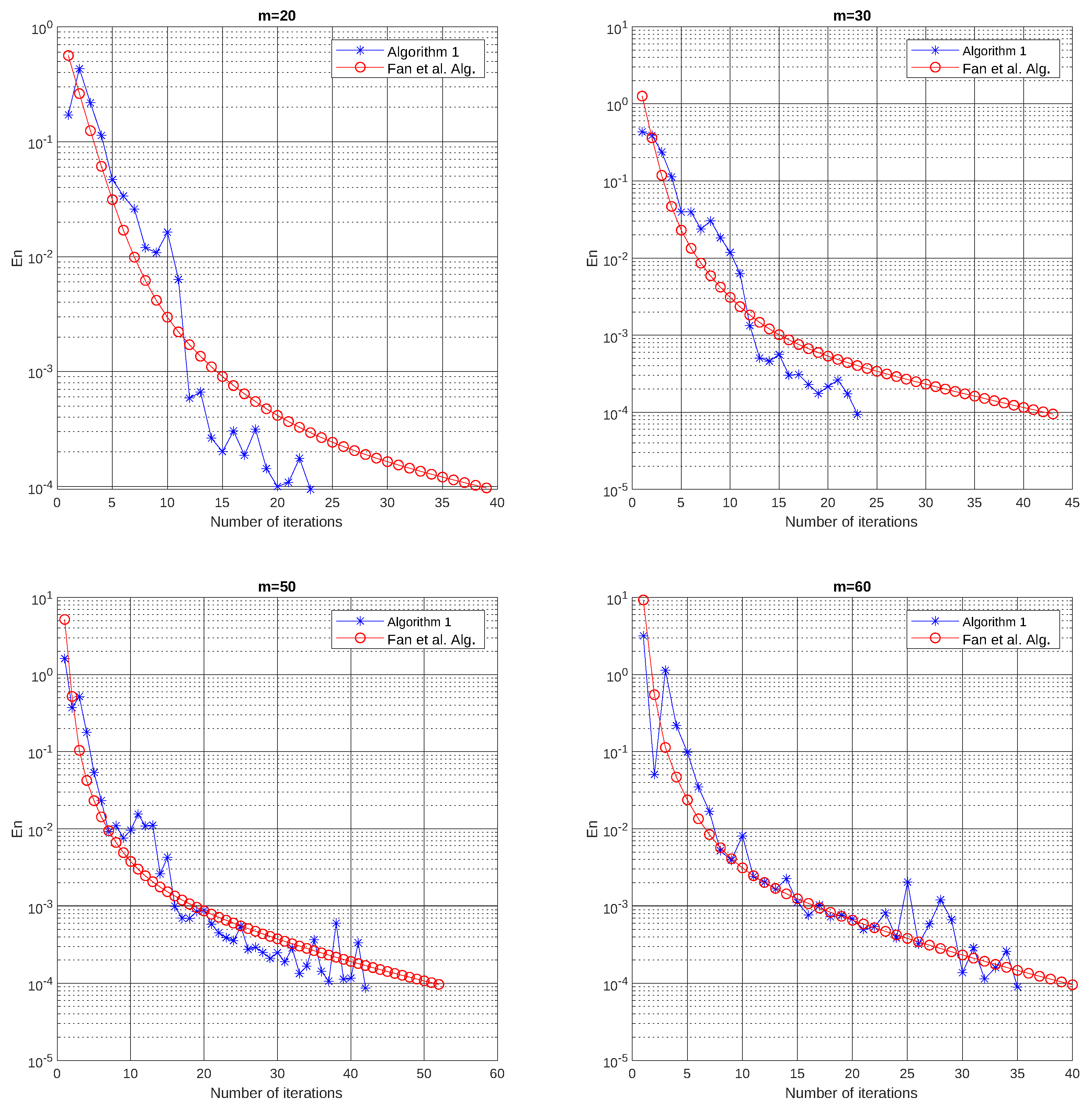
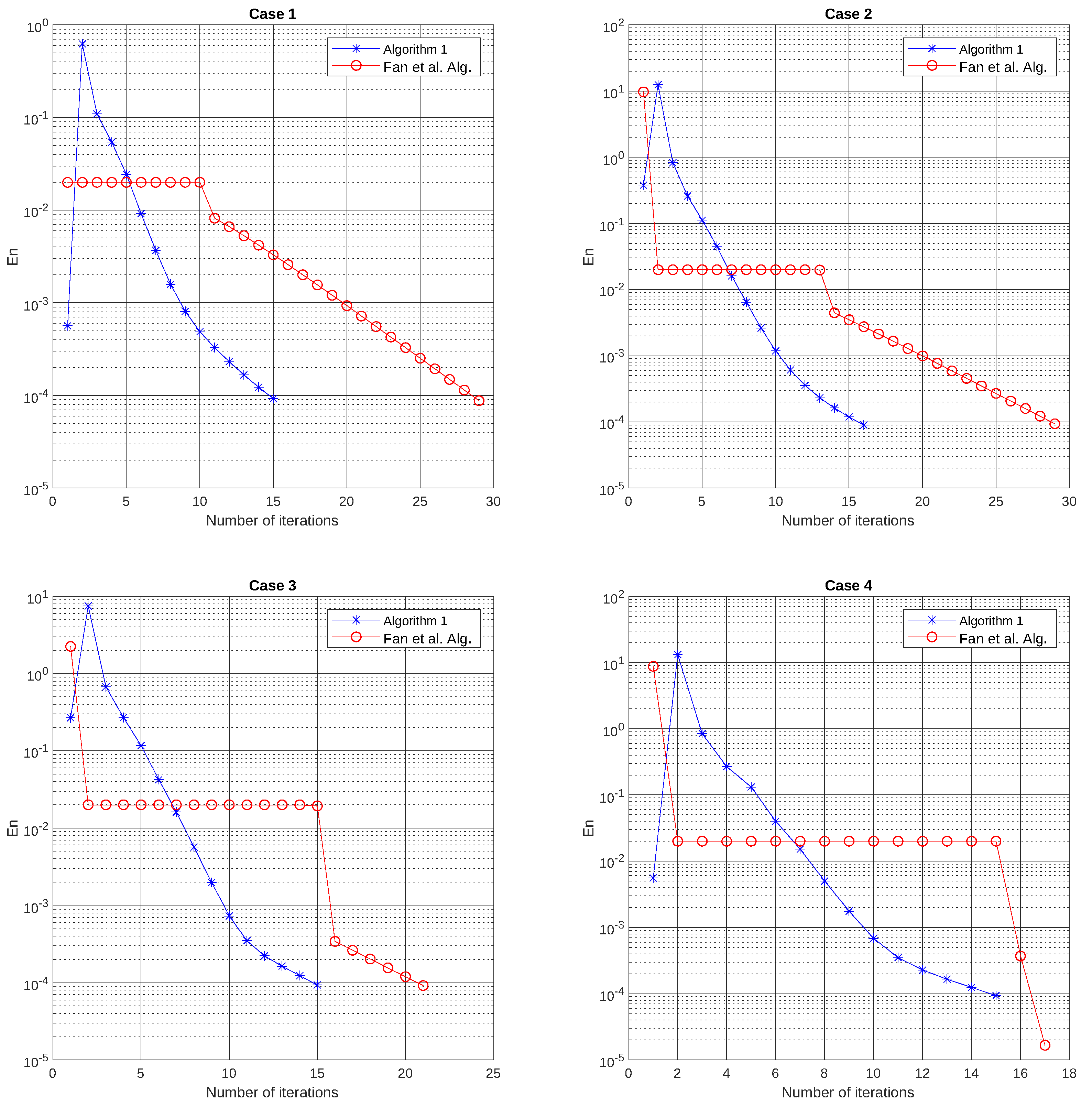
5. Numerical Example

In this section, we present some numerical illustrations of our main result. All codes were written in Matlab 2017b computed on a Personal Computer (PC) Core i5 at 2.0 GHz and 8.00 GB RAM.

Example 1.

We consider an extension of the Nash equilibrium model introduced in [7,47]. In this problem, the bifunction $g:K\times K\to \mathbb{R}$ is given by

$$g(x,y)=\langle Px+Qy+p,y-x\rangle .$$

Let M be Space 2 above and let $K\subset M$ be given by

$$K=\{x=(x_1,x_2,\cdots ,x_m):1\le x_i\le 100,i=1,2,\cdots ,m\}.$$

Let $x,y\in K,$ and let $p={(p_1,p_2,\cdots ,p_m)}^T\in {\mathbb{R}}^m$ be chosen randomly with elements in $[1,m]$. The matrices P and Q are two square matrices of order m such that Q is symmetric positive semidefinite and $Q-P$ is negative semidefinite. It is known (see [7]) that g is pseudomonotone and satisfies (A2) with Lipschitz constants $c_1=c_2=\frac{1}{2}\parallel Q-P\parallel$ (see [15], Lemma 6.2). Assumptions (A3) and (A4) are also satisfied (see [48]). Thus, our main theorem is fully compatible with this example. Setting ${\delta }_n=\frac{1}{2n+7},$ ${\beta }_n=\frac{1}{n+1},$ ${ϵ}_n=\frac{1}{n^{1.1}},$ $\mu =0.5$ and ${\lambda }_1={10}^{-3}$, we compare our method with (Algorithm 1) of Fan et al. [23]. The comparisons are made for some values of m using $\parallel x_{n+1}-x_n{\parallel }^2={10}^{-4}$ as the stopping criterion. The results for this example are presented in

Table 1. Computation results for Example 1.

		Algorithm 1	Fan et al. Alg.
$m=20$	No of Iter.	23	39
	CPU time (s)	0.0013	2.9229
$m=30$	No of Iter.	23	43
	CPU time (s)	0.0130	3.6771
$m=50$	No of Iter.	41	53
	CPU time (s)	0.0050	5.8712
$m=60$	No of Iter.	35	40
	CPU time (s)	0.0050	5.8712

and Figure 1.

Example 2.

Let M be Space 2 above. We consider an example of a variational inequality and present a numerical comparison of Algorithm 1 through its adaptation to VI with (Algorithm 1) of Fan et al. [23]. The following example has been considered by authors in many recent articles (see, for example, [49]). Let the mapping $F:E\to M$ be defined by

$$\begin{array}{c}\hfill F\left(x\right)=\left(\begin{array}{c}0.5x_1{x}_2-2x_2-{10}^7\\ -4x_1+0.1x_2^2-{10}^7\end{array}\right)\end{array}$$

where $x=(x_1,x_2)$ and $K:=\{x\in {\mathbb{R}}^2:{(x_1-2)}^2+{(x_2-2)}^2\le 1\}.$ It is known that the mapping F is pseudomonotone on K and L-Lipschitz continuous with $L=5.$ For this example, we let ${\beta }_n=\frac{1}{n+1},$ ${\delta }_n=\frac{1}{2n+1},$ ${\theta }_n=\frac{1}{3}$ and ${ϵ}_n=\frac{1}{n^{1.2}}$ and ${\lambda }_1={10}^{-8}$. Using $\parallel x_{n+1}-x_n{\parallel }^2={10}^{-4}$ as the stopping criterion, we compare Algorithm 1 and Fan et al. alg. for different initial values of $x_0$ and $x_1$. The results for this example are presented in Figure 2 and

Table 2. Computation result for Example 2.

		Algorithm 1	Fan et al. Alg.
Case 1	No of Iter.	15	29
	CPU time (s)	0.0013	2.9229
Case 2	No of Iter.	17	29
	CPU time (s)	0.0130	3.6771
Case 3	No of Iter.	15	22
	CPU time (s)	0.0050	5.8712
Case 4	No of Iter.	15	17
	CPU time (s)	0.0050	5.8712

.

(Case 1) 

$x_0=[0.5,1]$ and $x_1={[1,2]}^{\prime };$

(Case 2) 

$x_0=[2,-1]$ and $x_1={[1,-2]}^{\prime };$

(Case 3) 

$x_0=[1.2,1.5]$ and $x_1={[0,0.5]}^{\prime };$

(Case 4) 

$x_0=[0.3,0.5]$ and $x_1={[-0.9,-0.7]}^{\prime }.$

6. Conclusions

In this paper, we introduced an inertial subgradient extragradient method for approximating solutions to equilibrium problems in the framework of Hadamard manifolds. Since we use self-adaptive step sizes which are allowed to increase from iteration to iteration, our method does not require knowledge of the Lipschitz constant of the cost operator. A convergence result was proved by using a viscosity technique with mild conditions on the control parameters involved for generating the sequence of the approximants. We also provided two theoretical applications of our result. Furthermore, we presented some numerical experiments which illustrate the performance of the method we proposed. By way of comparison to another method presented for the same subject in Fan et al. [23], we displayed the competitiveness of our Algorithm. The authors intend to consider more examples in Hadamard manifolds in future works.

References

1. Fan, K. A Minimax Inequality and Its Application. In Inequalities; Shisha, O., Ed.; Academic: New York, NY, USA, 1972; Volume 3, pp. 103–113. [Google Scholar]
2. Blum, E.; Oettli, W. From optimization and variational inequalities to equilibrium problems. Math. Stud. 1994, 63, 123–145. [Google Scholar]
3. Muu, L.; Oettli, W. Convergence of an adaptive penalty scheme for finding constrained equilibria. Nonlinear Anal. 1992, 18, 1159–1166. [Google Scholar] [CrossRef]
4. Rapcsák, T. Geodesic convexity in nonlinear optimization. J. Optim. Theory Appl. 1991, 69, 169–183. [Google Scholar] [CrossRef]
5. Rapcsák, T. Nonconvex Optimization and Its Applications, Smooth Nonlinear Optimization in Rn; Kluwer Academic Publishers: Dordrecht, The Netherlands, 1997. [Google Scholar]
6. Udriste, C. Convex Functions and Optimization Methods on Riemannian Manifolds, Mathematics and Its Applications; Kluwer Academic: Norwell, MA, USA, 1994; Volume 297. [Google Scholar]
7. Khammahawong, K.; Kumam, P.; Chaipunya, P.; Yao, J.; Wen, C.; Jirakitpuwapat, W. An extragradient algorithm for strongly pseudomonotone equilibrium problems on Hadamard manifolds. Thai J. Math. 2020, 18, 350–371. [Google Scholar]
8. Upadhyay, B.; Ghosh, A.; Mishra, P.; Treanţă, S. Optimality conditions and duality for multiobjective semi-infinite programming problems on Hadamard manifolds using generalized geodesic convexity. RAIRO-Oper. Res. 2022, 56, 2037–2065. [Google Scholar] [CrossRef]
9. Colao, V.; López, G.; Marino, G.; Martín-Márquez, V. Equilibrium problems in Hadamard manifolds. J. Math. Anal. Appl. 2012, 388, 61–77. [Google Scholar] [CrossRef] [Green Version]
10. Salahuddin, S. The existence of solution for equilibrium problems in Hadamard manifolds. Trans. A. Razmadze Math. Inst. 2017, 171, 381–388. [Google Scholar] [CrossRef]
11. Tang, G.; Zhou, L.; Huang, N. Existence results for a class of hemivariational inequality problems on Hadamard manifolds. Optimization 2016, 65, 1451–1461. [Google Scholar] [CrossRef]
12. Zhou, L.-W.; Huang, N.-J. Existence of solutions for vector optimization on Hadamard manifolds. J. Optim. Theory Appl. 2013, 157, 44–53. [Google Scholar] [CrossRef]
13. Korpelevich, G. An extragradient method for finding saddle points and for other problems. Ekon. Mat. Metody. 1976, 12, 747–756. [Google Scholar]
14. Censor, Y.; Gibali, A.; Reich, S. The subgradient extragradient method for solving variational inequalities in Hilbert spaces. J. Optim. Theory Appl. 2011, 148, 318–335. [Google Scholar] [CrossRef] [PubMed] [Green Version]
15. Tran, D.; Dung, M.; Nguyen, V. Extragradient algorithms extended to equilibrium problems. Optimization 2008, 57, 749–776. [Google Scholar] [CrossRef]
16. Nguyen, T.; Strodiot, J.; Nguyen, V. Hybrid methods for solving simultaneously an equilibrium problem and countably many fixed point problems in a Hilbert space. J. Optim. Theory Appl. 2014, 160, 809–831. [Google Scholar] [CrossRef]
17. Rehman, H.; Kumam, P.; Sitthithakerngkiet, K. Viscosity-type method for solving pseudomonotone equilibrium problems in a real Hilbert space with applications. AIMS Math. 2021, 6, 1538–1560. [Google Scholar] [CrossRef]
18. Ceng, L.; Li, X.; Qin, X. Parallel proximal point methods for systems of vector optimization problems on Hadamard manifolds without convexity. Optimization 2020, 69, 357–383. [Google Scholar] [CrossRef]
19. Hieu, D.V.; Quy, P.K.; Vy, L.V. Explicit iterative algorithms for solving equilibrium problems. Calcolo 2019, 56, 11. [Google Scholar] [CrossRef]
20. Li, C.; López, G.; Martín-Márquez, V. Monotone vector fields and the proximal point algorithm on Hadamard manifolds. J. Lond. Math. Soc. 2009, 79, 663–683. [Google Scholar] [CrossRef]
21. Li, C.; Yao, J. Variational inequalities for set-valued vector fields on Riemannian manifolds: Convexity of the solution set and the proximal point algorithm. SIAM J. Control Optim. 2012, 50, 2486–2514. [Google Scholar] [CrossRef]
22. Neto, J.C.; Santos, P.; Soares, P. An extragradient method for equilibrium problems on Hadamard manifolds. Optim. Lett. 2016, 10, 1327–1336. [Google Scholar] [CrossRef]
23. Fan, J.; Tan, B.; Li, S. An explicit extragradient algorithm for equilibrium problems on Hadamard manifolds. Comp. Appl. Math. 2021, 40, 68. [Google Scholar] [CrossRef]
24. Ali-Akbari, M. A subgradient extragradient method for equilibrium problems on Hadamard manifolds. Int. J. Nonlinear Anal. Appl. 2022, 13, 75–84. [Google Scholar]
25. Alvarez, F.; Attouch, H. An inertial proximal method for maximal monotone operators via discretization of a nonlinear oscillator with damping. Set-Valued Anal. 2001, 9, 3–11. [Google Scholar] [CrossRef]
26. Polyak, B. Some methods of speeding up the convergence of iterarive methods. Zh. Vychisl. Mat. Mat. Fiz. 1964, 4, 1–17. [Google Scholar]
27. Rehman, H.; Kumam, P.; Gibali, A.; Kumam, W. Convergence analysis of a general inertial projection-type method for solving pseudomonotone equilibrium problems with applications. J. Ineq. Appl. 2021, 2021, 63. [Google Scholar] [CrossRef]
28. Oyewole, O.; Izuchukwu, C.; Okeke, C.; Mewomo, O. Inertial approximation method for split variational inclusion problem in Banach spaces. Int. J. Nonlinear Anal. Appl. 2020, 11, 285–304. [Google Scholar]
29. Moudafi, A. Viscosity approximation methods for fixed-points problems. J. Math. Anal. Appl. 2000, 241, 46–55. [Google Scholar] [CrossRef] [Green Version]
30. Al-Homidan, S.; Ansari, Q.; Babu, F.; Yao, J.-C. Viscosity method with a f-contraction mapping for hierarchical variational inequalities on Hadamard manifolds. Fixed Point Theory 2020, 21, 561–584. [Google Scholar] [CrossRef]
31. Huang, S. Approximations with weak contractions in Hadamard manifolds. Linear Nonlinear Anal. 2015, 1, 317–328. [Google Scholar]
32. Dilshad, M.; Khan, A.; Akram, M. Splitting type viscosity methods for inclusion and fixed point problems on Hadamard manifolds. AIMS Math. 2021, 6, 5205–5221. [Google Scholar] [CrossRef]
33. Thong, D.; Hieu, D. Some extragradient-viscosity algorithms for solving variational inequality problems and fixed point problems. Numer. Algorithms 2019, 82, 761–789. [Google Scholar] [CrossRef]
34. Sakai, T. Riemannian Geometry. Vol. 149, Translations of Mathematical Monographs; American Mathematical Society: Providence, RI, USA, 1996. [Google Scholar]
35. Ansari, Q.; Babu, F.; Yao, J. Regularization of proximal point algorithms in Hadamard manifolds. J. Fixed Point Theory Appl. 2019, 21, 25. [Google Scholar] [CrossRef]
36. Ferreira, O.; Perez, L.L.; Nemeth, S. Singularities of monotone vector fields and an extragradient algorithm. J. Glob. Optim. 2005, 31, 133–151. [Google Scholar] [CrossRef]
37. Wang, J.; López, G.; Martín-Márquez, V.; Li, C. Monotone and accretive vector fields on Riemannian manifolds. J. Optim. Theory Appl. 2010, 146, 691–708. [Google Scholar] [CrossRef] [Green Version]
38. Boyd, D.; Wong, J. On nonlinear contractions. Proc. Am. Math. Soc. 1969, 20, 335–341. [Google Scholar] [CrossRef]
39. Bridson, M.; Haefliger, A. Metric Spaces of Non-Positive Curvature. Grundlehren der Mathematischen Wissenschaften (Fundamental Principles of Mathematical Sciences); Springer: Berlin, Germany, 1999; Volume 319. [Google Scholar] [CrossRef]
40. Mastroeni, G. On auxiliary principle for equilibrium problems. In Equilibrium Problems and Variational Models; Nonconvex Optimization and Its Applications; Kluwer Academic: Norwell, MA, USA, 2003; Volume 68, pp. 289–298. [Google Scholar]
41. Ferreira, O.; Oliveira, P. Proximal Point Algorithm on Riemannian Manifolds. Optimization 2002, 51, 257–270. [Google Scholar] [CrossRef]
42. Takahashi, W. Introduction to Nonlinear and Convex Analysis; Yokohama Publishers: Yokohama, Japan, 2009. [Google Scholar]
43. Saejung, S.; Yotkaew, P. Approximation of zeros of inverse strongly monotone operator in Banach spaces. Nonlinear Anal. 2012, 75, 742–750. [Google Scholar] [CrossRef]
44. Stampacchia, G. Formes Bilineaires Coercivites sur les Ensembles Convexes. C. R. Acad. Paris 1964, 258, 4413–4416. [Google Scholar]
45. Upadhyay, B.; Treanţă, S.; Mishra, P. On Minty Variational Principle for Nonsmooth Multiobjective Optimization Problems on Hadamard Manifolds. Optimization 2022, 71, 1–19. [Google Scholar] [CrossRef]
46. Cegielski, A. Iterative Methods for Fixed Point Problems in Hilbert Spaces; Lecture Notes in Mathematics; 2057; Springer: Berlin, Germany, 2012. [Google Scholar]
47. Facchinei, F.; Pang, J.S. Finite-Dimensional Variational Inequalities and Complementarity Problems; Springer Series in Operations Research; Springer: New York, NY, USA, 2003; Volume II. [Google Scholar]
48. Chen, J.; Liu, S. Extragradient-like method for pseudomonotone equilibrium problems on Hadamard manifolds. J. Ineq. Appl. 2020, 2020, 205. [Google Scholar] [CrossRef]
49. Shehu, Y.; Dong, Q.-L.; Jiang, D. Single projection method for pseudo-monotone variational inequality in Hilbert Spaces. Optimization 2019, 68, 385–409. [Google Scholar] [CrossRef]
Figure 1. Example 1, Top left: m = 20 ; Top right: m = 30 ; Bottom left: m = 50 ; Bottom right: m = 60 .
Axioms 12 00256 g001
Figure 2. Example 2, Top left: Case 1; Top right: Case 2; Bottom left: Case 3; Bottom right: Case 4.
Axioms 12 00256 g002