Parameter Estimation Analysis in a Model of Honey Production

Abstract

Honeybee losses are an extensive global problem. In this study, a new compartment model of honeybee population that mainly concerns honey production is developed. The model describes the interaction of the food stock with the brood (immature bees), adult bees and produced honey. In the present paper, the issue of an adequate model recovery is addressed and the parameter identification inverse problem is solved. An adjoint equation procedure to obtain the unknown parameter values by minimizing the functional error during a period of time is proposed. Numerical simulations with realistic data are discussed.

1. Introduction

Honeybee colonies are important for agriculture and the environment. They help plant reproduction by pollination, while beekeeping redounds to the development of rural areas. Unfortunately, in recent decades, a ubiquitous decline in both managed and unmanaged colonies has been observed. This is a global problem, since the bees contribute to the ecological equilibrium. If the bee population shrinks or disappears, plants would not get pollinated and would die off. Then, herbivorous animals would not have food and would go extinct, and they would be followed by carnivorous animals, including humans. Thus, preventing bee colonies from losses is of a paramount importance for preserving live on Earth in general.

Of the many species of bees, only a small number of them are eusocial; Apis mellifera is an example of eusocial behavior [1]. This species form colonies thus the survival, reproduction and honey production are directly dependent on the size and the structure of the colonies [2].

Honey, produced by honeybees, is a sweet natural substance, derived greatly from the nectar of flowers and transformed by a group of enzymes, which are present in the saliva of the worker bees. The honey is also airy and evaporates by its filtering, and is eventually stored inside the hives. Honey from Apis mellifera is one of the most essential zoo-agricultural goods for commercial trade in the world [3]. Regarding the honey trade, the USA is the global leader in imports. Concerning production, China is the global leader, following by Turkey, Iran, Ukraine and the Russian Federation. Finally, with respect to quality, Bulgarian honey is the most pure and sweet [4].

Beekeepers produce a variety of agriculture products, in addition to honey, including royal jelly, propolis and beeswax. This paper aims to develop mathematical modeling of the honeybee population dynamics and, therefore, honey production.

The most fundamental honeybee population model is suggested by [5], where only two compartments are explored—the young hive bees and the matured forager bees. This model is extended in [6,7], where the brood, the age of the foragers and the food are also included in the studies, accounting for the delay of maturing. Such investigation is done in [8], where a different form of the recruitment rate is used. In the study [9], exogenous stress is assumed to impact the recruitment process, social inhibition and the queen laying rate, causing a potential colony decline.

There are models developed as an effort to understand the decrease in colony numbers in recent decades. A survey in the USA suggests that treating against disease and mite infestation in the right way lowers the chance of colony loss [10]. Extensive study of the transition from hive to forager bees is performed in [11]. A comparison between the losses in different parts of the world is performed in [12].

The mysterious disease, whose causal factors are not entirely agreed on, is called Colony Collapse Disorder (CCD). It is characterized by rapid loss of forager bees but absence of dead bodies near the hive, lack of pest and mite invasion of the hive, and bees’ reluctance to consume food provided by the beekeeper. The first recorded massive colony loss is described as the ‘Isle of Wight Disease’ [13]. The effect of protein sources has been proposed as a potential cause for collapse [14]. A special CCD model is designed in [15], where the contagious adult bees are isolated from the others. A review of the suspected causal factors for the colony declines is summarized in [16].

Other models focus on particular parts of the surrounding environment such as food availability [17], age structure [18], seasonal effects [19], Varroa mites [20] and others [21,22], including the model memory property [23].

In [24], populations of adult and immature (brood) honeybees as well as their honeybee production are examined via mathematical and statistical modeling approaches. It is shown that, if a bee population is exposed to a stress factor (i.e., habitat destruction, Varroamites, climate variability, heavy metals, etc.), the number of individuals declines over time as well as the produced honey. The complex issue of the sustainability of honeybee colonies is important not only for the survival of the species but also for food security and the overall health of the environment. To ensure the sustainability of honeybee colonies, it is important to take measures such as providing adequate habitats, reducing pesticide exposure and promoting disease management practices. Aiming at the latter, the sophisticated processes of population dynamics have to be investigated via mathematical modeling.

In the present work we study the relationship between the population size of honeybees (Apis mellifera) and honey production if the bee colony is exposed to a number of stress factors that exogenously cause the death of individuals and therefore a possible reduction in honey production. Here lies the main originality of the study—suggesting a novel model for encountering the interaction between the bee castes and the amount of honey, stored in the hive.

Furthermore, in the investigation the inverse problem of identifying the food and honey consumption rates by the immature and adult bees is solved as well as the brood maturation rate. These quantities are of extreme importance for understanding the complex dynamics of the hive. It is done via the adjoint equations optimization approach. Such a study is performed in [25], where the contaminated bees are modeled as a separate compartment. Similar investigation is done in [26] but, for the coefficient identification, a trust-region reflexive algorithm is used.

This paper is organized as follows. In the next section, we extend the mathematical model, studied in [24], taking into account the food stock. What is more, we study the existence and non-negativity of the solutions. Section 3 is devoted to the parameter estimation analysis of the model. Section 4 is dedicated to numerical experiments regarding the direct and inverse problems. The paper is concluded in Section 5.

2. Mathematical Model

In this section, we introduce a mathematical model that explains the interaction between the food stock and the brood (immature bees), adult bees and the amount of produced honey.

Following the results in [24,27] we establish a mathematical model that presents the interactions among brood $B\left(t\right)$ at time t, adult bees $A\left(t\right)$ and the amount of honey production $M\left(t\right)$, taking into account the weight of food stock $F\left(t\right)$.

We assume that the brood grows at a rate $\beta$, proportionally to the number of adult bees. This is given by term $A/(A+\nu )$, where $\nu$ is the mean saturation rate (number of adult bees required for immature bees to achieve half of their maximal number). The number of bees surviving to the adult stage influences the number of immature bees.

The latter is modeled by the term $\omega B$, where $\omega$ denotes the maturation rate to adult stage, and $1/\omega$ indicates the time spent before achieving the adult stage. The number of immature bees is decreased by natural death and it is modeled by the term ${\mu }_{B}B$, where ${\mu }_B$ denotes the natural mortality rate of the immature stage. Following this discussion and those in [24,27] we consider the following system of ODEs:

$$\frac{\mathrm{d}F}{\mathrm{d}t}=cA-\gamma B,$$

(1)

$$\frac{\mathrm{d}B}{\mathrm{d}t}=\beta \frac{A}{A+\nu }-\omega B-{\mu }_{B}B,$$

(2)

$$\frac{\mathrm{d}A}{\mathrm{d}t}=\omega B-{\mu }_{A}A-\sigma A.$$

(3)

$$\frac{\mathrm{d}M}{\mathrm{d}t}=\rho \frac{A}{A+u}-\alpha M-\delta AM.$$

(4)

The model (1)–(4) is illustrated in the diagram of Figure 1.

It is assumed in the derivation of Equation (3) that the number of adult bees diminish naturally and it is demonstrated by the term ${\mu }_{A}A$, where ${\mu }_A$ is the natural mortality rate of the adult stage. However, the bees can also die because of a stress factor. This is represented by the term $\sigma A$, where $\sigma$ is the death rate due to a stressor (climate change, loss of habitat, heavy metals or pesticides, poor beekeeper’s management, etc.) acting on bees at the adult stage.

Equation (4) shows that the production of honey in hives increase at a rate $\rho$, which is influenced by the number of adult bees, given by the term $A/(A+u)$, where u is the mean saturation rate.

One important cause for decreasing of the honey is the feeding of immature bees, which is demonstrated by the term $\alpha M$, where $\alpha$ is the honey loss rate.

The term $\delta AM$ represents the loss of honey production because of the consumption of adult bees, where $\delta$ is the adult bees’ honey consumption rate.

For more details on the specifications of the parameters in the model we refer to Table 2 in [24].

We solve the system of ordinary differential Equations (1)–(4) with initial conditions

$$F\left(0\right)=F_0\ge 0,B\left(0\right)=B_0\ge 0,A\left(0\right)=A_0\ge 0,M\left(0\right)=M_0\ge 0.$$

(5)

Using Theorem 7.1 in [28] one could easily prove that the subsystem (2)–(4) is positive (short for “non-negativity preserving”) in the sense that, if

$$B\left(0\right)\ge 0,A\left(0\right)\ge 0,M\left(0\right)\ge 0,$$

then

$$B\left(t\right)\ge 0,A\left(t\right)\ge 0,M\left(t\right)\ge 0,\forall t\ge 0.$$

This property is biologically relevant to the model.

3. Parameter Identification

In this section, the parameter inverse problem is defined. Such problems appear very often in practice. The problem (1)–(5), where the values of the parameters are known, is well-posed and it is called a direct problem. However, in the real world, the values of some of the coefficients are not directly measurable but they are very important for professional honeybee management. Their reconstruction, provided that additional information is given, is referred to an inverse problem. Inverse problems are ill-posed and harder to solve. We employ the adjoint equation optimization approach [29,30].

The parameters to be reconstructed are $\mathit{p}=(p^1,p^2,p^3,p^4,p^5)$, $p^1=\alpha$, $p^2=\gamma$, $p^3=\delta$, $p^4=\sigma$, $p^5=\omega$, and

$$\mathit{p}\in {\mathbb{S}}_{\mathrm{adm}}=\left\{\mathit{p}\in {\mathbb{R}}^5:0<p^i<P^i,i=1,\dots ,5\right\}.$$

(6)

The admissible set ${\mathbb{S}}_{\mathrm{adm}}$ is defined by the biology of the honeybee [31]. To find the parameters $\mathit{p}$, though, some new information must be brought. In many cases it is possible to measure the model functions at some discrete times. In reality, counting the brood B is a difficult task, so we adopt measurements of the functions

$$\begin{array}{c}{F}^{\mathrm{obs}}\left(t_k\right)=X_k,\\ A^{\mathrm{obs}}\left(t_k\right)=Y_k,\\ M^{\mathrm{obs}}\left(t_k\right)=Z_k\end{array}$$

(7)

for $k=1,\dots ,K$. We assume all functions are measured at some predefined time instances. The observation times for every function may be different.

In practice, the observations are obtained from electronic devices equipping the hive. In a quasi-real setting, first the direct problem is solved and then the observations are extracted from the solution to the direct problem.

To solve the inverse problem, the least-square function

$$\begin{array}{c}\mathsf{\Phi }\left(\mathit{p}\right)=\mathsf{\Phi }(\alpha ,\gamma ,\delta ,\sigma ,\omega )={\mathsf{\Phi }}_F(\alpha ,\gamma ,\delta ,\sigma ,\omega )+{\mathsf{\Phi }}_A(\alpha ,\gamma ,\delta ,\sigma ,\omega )+{\mathsf{\Phi }}_M(\alpha ,\gamma ,\delta ,\sigma ,\omega )=\hfill \\ \hfill \sum _{k=1}^K{(F(t_k;\mathit{p})-X_k)}^2+\sum _{k=1}^K{(A(t_k;\mathit{p})-Y_k)}^2+\sum _{k=1}^K{(M(t_k;\mathit{p})-Z_k)}^2\end{array}$$

(8)

is minimized, e.g., by a gradient method [32], where $\mathsf{\Psi }(t_k;\mathit{p})$, $\mathsf{\Psi }\in \{F,A,M\}$ are the theoretical quantities from the model and ${\mathsf{\Xi }}_k$, $\mathsf{\Xi }\in \{X,Y,Z\}$ are the observed values in practice.

Now we state an expression for the gradient of the function ${\mathsf{\Phi }}_{\mathit{p}}:=\mathsf{\Phi }\left(\mathit{p}\right)$.

Theorem 1.

The gradient ${\mathsf{\Phi }}_{\mathit{p}}^{\prime }\equiv ({\mathsf{\Phi }}_{\alpha }^{\prime },{\mathsf{\Phi }}_{\gamma }^{\prime },{\mathsf{\Phi }}_{\delta }^{\prime },{\mathsf{\Phi }}_{\sigma }^{\prime },{\mathsf{\Phi }}_{\omega }^{\prime })$ is given by

$${\mathsf{\Phi }}_{\alpha }^{\prime }={\int }_0^T{\phi }_M\left(t\right)M\left(t\right)\mathrm{d}t,$$

(9)

$${\mathsf{\Phi }}_{\gamma }^{\prime }={\int }_0^T{\phi }_F\left(t\right)B\left(t\right)\mathrm{d}t,$$

(10)

$${\mathsf{\Phi }}_{\delta }^{\prime }={\int }_0^T{\phi }_M\left(t\right)A\left(t\right)M\left(t\right)\mathrm{d}t,$$

(11)

$${\mathsf{\Phi }}_{\sigma }^{\prime }={\int }_0^T{\phi }_A\left(t\right)A\left(t\right)\mathrm{d}t,$$

(12)

$${\mathsf{\Phi }}_{\omega }^{\prime }=-{\int }_0^T{\phi }_A\left(t\right)B\left(t\right)\mathrm{d}t,$$

(13)

where the triple $\{{\phi }_M,{\phi }_F,{\phi }_A\}$ is the unique solution of the adjoint system

$$\frac{\mathrm{d}{\phi }_F}{\mathrm{d}t}=2\sum _{k=1}^K(F-X)\delta (t-t_k),$$

(14)

$$\frac{\mathrm{d}{\phi }_A}{\mathrm{d}t}=-c{\phi }_F+({\mu }_A+\sigma ){\phi }_A+\left(\delta ·M-\rho \frac{u}{{(A+u)}^2}\right){\phi }_M+2\sum _{k=1}^K(A-Y)\delta (t-t_k),$$

(15)

$$\frac{\mathrm{d}{\phi }_M}{\mathrm{d}t}=(\alpha +\delta ·A){\phi }_M+2\sum _{k=1}^K(M-Z)\delta (t-t_k),$$

(16)

$${\phi }_F\left(T\right)={\phi }_A\left(T\right)={\phi }_M\left(T\right)=0.$$

(17)

Proof. 

We denote $\delta \mathit{p}=(\delta \alpha ,\delta \gamma ,\delta \delta ,\delta \sigma ,\delta \omega )$ and $\delta \alpha =\epsilon h_1$, $\delta \gamma =\epsilon h_2$, $\delta \delta =\epsilon h_3$, $\delta \sigma =\epsilon h_4$, $\delta \omega =\epsilon h_5$.

If $\delta F(t;\mathit{p})=F(t;\mathit{p}+\delta \mathit{p})-F(t;\mathit{p})$, $\delta A(t;\mathit{p})=A(t;\mathit{p}+\delta \mathit{p})-A(t;\mathit{p})$ and $\delta M(t;\mathit{p})=M(t;\mathit{p}+\delta \mathit{p})-M(t;\mathit{p})$, write the ODE system for $F(t;\mathit{p}+\delta \mathit{p})$, $A(t;\mathit{p}+\delta \mathit{p})$ and $M(t;\mathit{p}+\delta \mathit{p})$ as (1), (3) and (4) with initial conditions $F_0,A_0$ and $M_0$ (5).

Then, calculate the differences of the corresponding equations to obtain an ODE system for $\delta F,\delta A$ and $\delta M$ with zero initial conditions.

$$\frac{\mathrm{d}}{\mathrm{d}t}\delta F=c\delta A-\delta \gamma B,$$

(18)

$$\frac{\mathrm{d}}{\mathrm{d}t}\delta A=-({\mu }_A+\sigma )\delta A-\delta \sigma A+\delta wB,$$

(19)

$$\frac{\mathrm{d}}{\mathrm{d}t}\delta M=\rho \frac{u\delta A}{{(A+u)}^2}-\delta ·M\delta A-(\alpha +\delta ·A)\delta M-\delta \alpha M-\delta \delta AM.$$

(20)

We find the increment of the functional $\mathsf{\Phi }\left(\mathit{p}\right)$:

$$\begin{array}{c}\mathsf{\Phi }(\mathit{p}+\delta \mathit{p})-\mathsf{\Phi }\left(\mathit{p}\right)=2\sum _{k=1}^K\delta F(t_k;\mathit{p})\left(F(t_k;\mathit{p})-X_k\right)\hfill \\ +2\sum _{k=1}^K\delta A(t_k;\mathit{p})\left(A(t_k;\mathit{p})-Y_k\right)+2\sum _{k=1}^K\delta M(t_k;\mathit{p})\left(M(t_k;\mathit{p})-Z_k\right)\hfill \\ =2\sum _{k=1}^K{\int }_0^T\delta F(t_k;\mathit{p})\left(F(t_k;\mathit{p})-X_k\right)\delta (t-t_k)\mathrm{d}t\\ +2\sum _{k=1}^K{\int }_0^T\delta A(t_k;\mathit{p})\left(A(t_k;\mathit{p})-Y_k\right)\delta (t-t_k)\mathrm{d}t\\ \hfill +2\sum _{k=1}^K{\int }_0^T\delta M(t_k;\mathit{p})\left(M(t_k;\mathit{p})-Z_k\right)\delta (t-t_k)\mathrm{d}t.\end{array}$$

Let us multiply Equations (18)–(20) by smooth functions ${\phi }_F\left(t\right)$, ${\phi }_A\left(t\right)$ and ${\phi }_M\left(t\right)$ s.t. ${\phi }_F\left(T\right)={\phi }_A\left(T\right)={\phi }_M\left(T\right)=0$ and integrate both sides of the results from 0 to T:

$$\begin{array}{c}{\displaystyle {\int }_0^T\left({\phi }_F\frac{\mathrm{d}}{\mathrm{d}t}\delta F+{\phi }_A\frac{\mathrm{d}}{\mathrm{d}t}\delta A+{\phi }_M\frac{\mathrm{d}}{\mathrm{d}t}\delta M\right)\mathrm{d}t=}\\ {\displaystyle c{\int }_0^T{\phi }_F\delta A\mathrm{d}t-\delta \gamma {\int }_0^T{\phi }_{F}B\mathrm{d}t-({\mu }_A+\sigma ){\int }_0^T{\phi }_A\delta A\mathrm{d}t}\\ {\displaystyle -\delta \sigma {\int }_0^T{\phi }_{A}A\mathrm{d}t+\delta w{\int }_0^T{\phi }_{A}B\mathrm{d}t+\rho u{\int }_0^T{\phi }_M\frac{\delta A}{{(A+u)}^2}\mathrm{d}t}\\ {\displaystyle -\delta {\int }_0^T{\phi }_{M}M\delta A\mathrm{d}t-(\alpha +\delta ·A){\int }_0^T{\phi }_M\delta M\mathrm{d}t}\\ {\displaystyle -\delta \alpha {\int }_0^T{\phi }_{M}M\mathrm{d}t-\delta \delta {\int }_0^T{\phi }_{M}AM\mathrm{d}t.}\end{array}$$

(21)

On the other hand, integrating by parts and using the facts that ${\phi }_F\left(T\right)={\phi }_A\left(T\right)={\phi }_M\left(T\right)=0$ and $\delta F\left(0\right)=\delta A\left(0\right)=\delta M\left(0\right)=0$, we obtain

$$\begin{array}{c}{\displaystyle {\int }_0^T{\phi }_F\frac{\mathrm{d}}{\mathrm{d}t}\delta F\mathrm{d}t+{\int }_0^T{\phi }_A\frac{\mathrm{d}}{\mathrm{d}t}\delta A\mathrm{d}t+{\int }_0^T{\phi }_M\frac{\mathrm{d}}{\mathrm{d}t}\delta M\mathrm{d}t=}\\ {\displaystyle -{\int }_0^T\delta F\frac{\mathrm{d}{\phi }_F}{\mathrm{d}t}\mathrm{d}t-{\int }_0^T\delta A\frac{\mathrm{d}{\phi }_A}{\mathrm{d}t}\mathrm{d}t-{\int }_0^T\delta M\frac{\mathrm{d}{\phi }_M}{\mathrm{d}t}\mathrm{d}t.}\end{array}$$

(22)

Let us place the expressions for $\frac{\mathrm{d}{\phi }_F}{\mathrm{d}t},\frac{\mathrm{d}{\phi }_A}{\mathrm{d}t}$ and $\frac{\mathrm{d}{\phi }_M}{\mathrm{d}t}$ from (14)–(16) in (22):

$$\begin{array}{c}{\displaystyle {\int }_0^T\left({\phi }_F\frac{\mathrm{d}}{\mathrm{d}t}\delta F+{\phi }_A\frac{\mathrm{d}}{\mathrm{d}t}\delta A+{\phi }_M\frac{\mathrm{d}}{\mathrm{d}t}\delta M\right)\mathrm{d}t=}\hfill \\ {\displaystyle c{\int }_0^T{\phi }_F\delta A\mathrm{d}t-({\mu }_A+\sigma ){\int }_0^T{\phi }_A\delta A\mathrm{d}t-\delta {\int }_0^T{\phi }_{M}M\delta A\mathrm{d}t}\\ +\rho u{\int }_0^T{\phi }_M\frac{1}{{(A+u)}^2}\delta A\mathrm{d}t-(\alpha +\delta ·A){\int }_0^T{\phi }_M\delta M\mathrm{d}t\\ {\displaystyle -2{\int }_0^T\delta F\sum _{k=1}^K(F-X)\delta (t-t_k)\mathrm{d}t-2{\int }_0^T\delta A\sum _{k=1}^K(A-Y)\delta (t-t_k)\mathrm{d}t}\\ \hfill {\displaystyle -2{\int }_0^T\delta M\sum _{k=1}^K(M-Z)\delta (t-t_k)\mathrm{d}t.}\end{array}$$

(23)

Equating (21) and (23) yields

$$\begin{array}{c}{\displaystyle 2{\int }_0^T\delta F\sum _{k=1}^K(F-X)\delta (t-t_k)\mathrm{d}t+2{\int }_0^T\delta A\sum _{k=1}^K(A-Y)\delta (t-t_k)\mathrm{d}t}\hfill \\ {\displaystyle +2{\int }_0^T\delta M\sum _{k=1}^K(M-Z)\delta (t-t_k)\mathrm{d}t=\delta \alpha {\int }_0^T{\phi }_{M}M\mathrm{d}t}\\ {\displaystyle +\delta \gamma {\int }_0^T{\phi }_{F}B\mathrm{d}t+\delta \delta {\int }_0^T{\phi }_{M}AM\mathrm{d}t}\\ \hfill +\delta \sigma {\int }_0^T{\phi }_{A}A\mathrm{d}t-\delta \omega {\int }_0^T{\phi }_{A}B\mathrm{d}t.\end{array}$$

Rewriting the last expression give

$$\begin{array}{c}\mathsf{\Phi }(\alpha +\epsilon h_1,\gamma +\epsilon h_2,\delta +\epsilon h_3,\sigma +\epsilon h_4,w+\epsilon h_5)-\mathsf{\Phi }(\alpha ,\gamma ,\delta ,\sigma ,\omega )=\hfill \\ \hfill \left(h_1{\int }_0^{\tau }{\phi }_{M}M\mathrm{d}t+h_2{\int }_0^{\tau }{\phi }_{F}B\mathrm{d}t+h_3{\int }_0^{\tau }{\phi }_{M}AM\mathrm{d}t+h_4{\int }_0^{\tau }{\phi }_{A}A\mathrm{d}t-h_5{\int }_0^{\tau }{\phi }_{A}B\mathrm{d}t\right)\epsilon .\end{array}$$

Now, taking $h_2=h_3=h_4=h_5=0$, dividing both sides by $\epsilon h_1$ and taking the limit $\epsilon \to 0$ we find the formula for ${\mathsf{\Phi }}_{\alpha }^{\prime }$ in the theorem.

Analogously, we obtain the formulae for ${\mathsf{\Phi }}_{\gamma }^{\prime }$, ${\mathsf{\Phi }}_{\delta }^{\prime }$, ${\mathsf{\Phi }}_{\sigma }^{\prime }$ and ${\mathsf{\Phi }}_{\omega }^{\prime }$ (10)–(13). □

Employing the fundamental property of the Dirac-delta function ${\displaystyle {\int }_0^T\mathfrak{f}\left(t\right)\delta (t-t_k)\mathrm{d}t=\mathfrak{f}\left(t_k\right)}$, $t_k\in (0,T)$, where $\mathfrak{f}\left(t\right)$ is a continuous function, (14)–(17) could be rewritten in its equivalent form:

$$\begin{array}{c}{\displaystyle \frac{\mathrm{d}{\phi }_F}{\mathrm{d}t}=0,t\ne t_k,k=1,\dots ,K,}\hfill \\ {\displaystyle \frac{\mathrm{d}{\phi }_A}{\mathrm{d}t}=-c{\phi }_F+({\mu }_A+\sigma ){\phi }_A+\left(\delta ·M-\rho \frac{u}{{(A+u)}^2}\right){\phi }_M,t\ne t_k,k=1,\dots ,K,}\hfill \\ {\displaystyle \frac{\mathrm{d}{\phi }_M}{\mathrm{d}t}=(\alpha +\delta ·A){\phi }_M,t\ne t_k,k=1,\dots ,K,}\hfill \\ {\left[{\phi }_F\right]}_{t=t_k}=2\left(F(t_k;\mathit{p})-X_k\right),k=1,\dots ,K,\hfill \\ {\left[{\phi }_A\right]}_{t=t_k}=2\left(A(t_k;\mathit{p})-Y_k\right),k=1,\dots ,K,\hfill \\ {\left[{\phi }_M\right]}_{t=t_k}=2\left(M(t_k;\mathit{p})-Z_k\right),k=1,\dots ,K,\hfill \\ {\phi }_F\left(T\right)={\phi }_A\left(T\right)={\phi }_M\left(T\right)=0.\hfill \end{array}$$

Having obtained the gradient, we employ an iterative procedure as follows, where the new approximation ${\mathit{p}}_{s+1}$ is defined by

$${\mathit{p}}_{s+1}={\mathit{p}}_s-\mathit{r}{\mathsf{\Phi }}^{\prime }\left({\mathit{p}}_s\right),$$

(24)

where $\mathit{r}\in {\mathbb{R}}_5^{+}$ are gradient multipliers. The iterations start at chosen ${\mathit{p}}_0$ and end if $∥▵{\mathit{p}}_s∥:=∥{\mathit{p}}_{s+1}-{\mathit{p}}_s∥<{\epsilon }_{\mathit{p}}$, where ${\epsilon }_{\mathit{p}}$ is a tolerance quantity, else increase $s:=s+1$ and start a new iteration. The final approximation is denoted with $\check{\mathit{p}}$ and it is called a nonlinear estimator.

4. Numerical Experiments

This section is devoted to presenting numerical tests which demonstrate the algorithm application. Firstly, the numerical algorithm is summarized. Then, the direct problem is solved and its solution is used to obtain measurements for the inverse problem.

4.1. Numerical Procedure

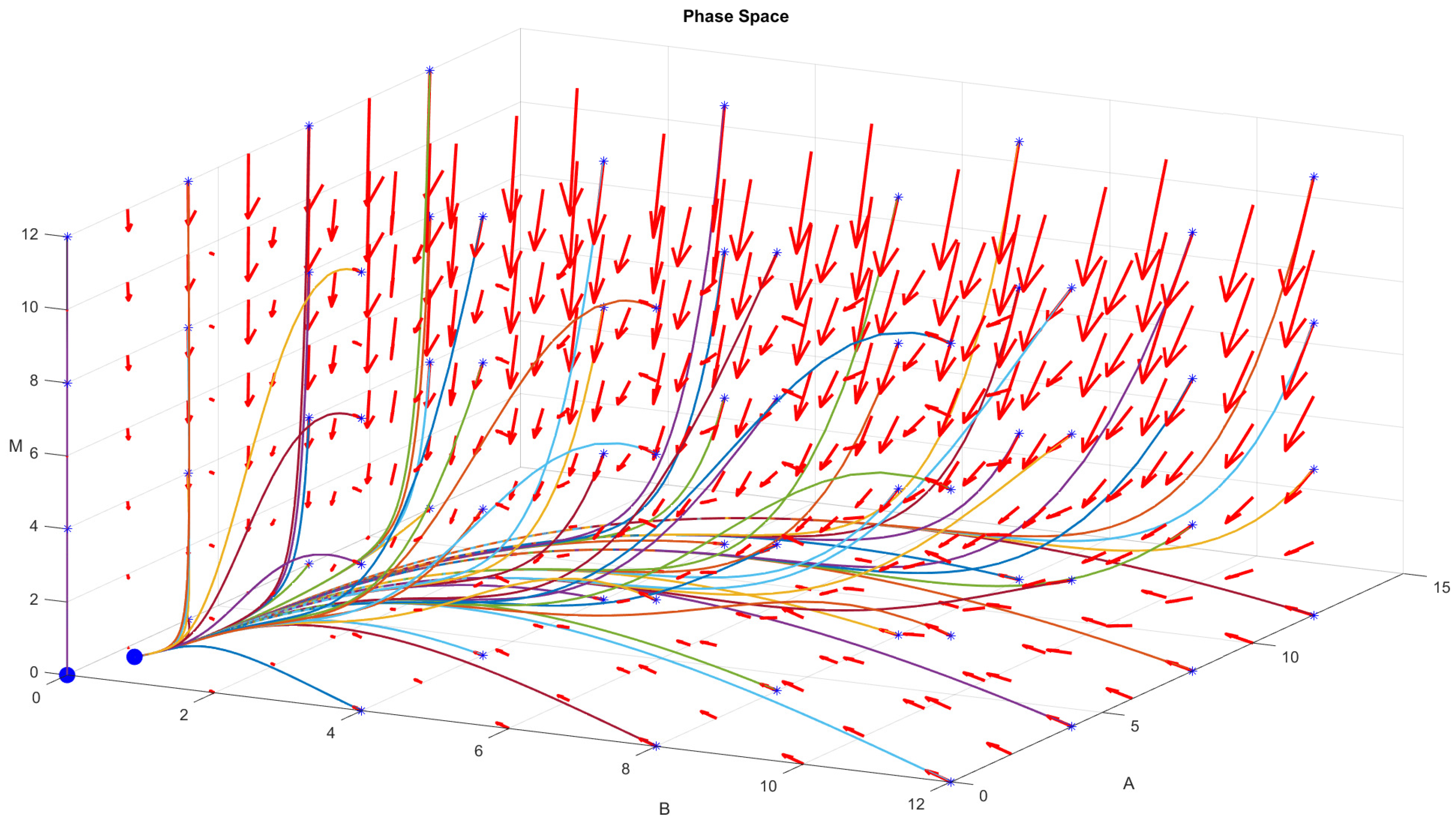
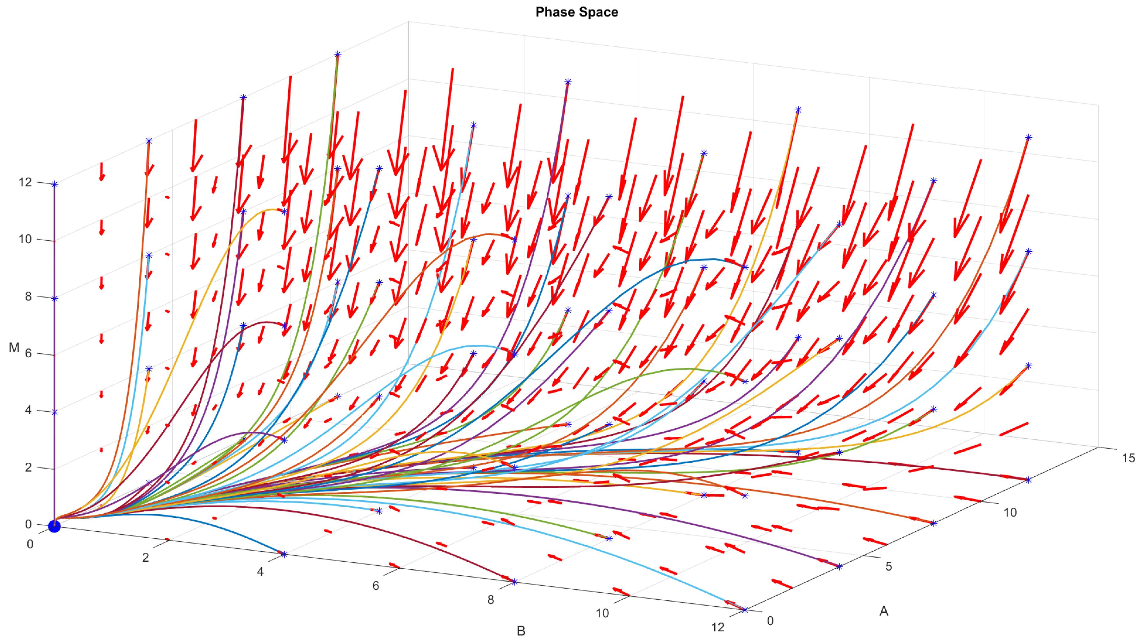
All the programming code is implemented in the MATLAB^® environment. For solving the ODE systems (1)–(5) and (14)–(17), a Runge–Kutta-type method is used. The algorithm for solving the inverse problem could be described as follows:

• Choose initial approximation ${\mathit{p}}_0$.
• Set $s:=0$.
• Until $∥▵{\mathit{p}}_s∥<{\epsilon }_{\mathit{p}}$ do

  3.1.

  Solve system (1)–(5) with ${\mathit{p}}_s$ to obtain F, B, A and M.

  3.2.

  Solve system (14)–(17) to obtain ${\phi }_F$, ${\phi }_A$ and ${\phi }_M$.

  3.3.

  Compute the gradient ${\mathsf{\Phi }}_{\mathit{p}}^{\prime }$ (9)–(13).

  3.4.

  Calculate ${\mathit{p}}_{s+1}$ by (24) and set $s:=s+1$.

• The estimator is set to $\check{\mathit{p}}:={\mathit{p}}_s$.

4.2. Direct Problem

Let us first solve the direct problem (1)–(5) with realistic data given in [24,27]. The adult food collection rate is assumed to be $c=0.04$ g/bee/day. The larval consumption rate is $\gamma =0.12$ g/bee/day. The brood reproduction rate is $\beta =0.92$ bee/day. The adult maturation rate is $\omega =0.95$ day⁻¹. The brood natural mortality rate is ${\mu }_B=0.11$ day⁻¹. The adult bee natural mortality rate is ${\mu }_A=0.29$ day⁻¹. The adult bee stressor mortality rate is $\sigma =0.1$ day⁻¹. The honey production rate is $\rho =0.23$ bees/day. The rate of natural honey loss is $\alpha =0.018$ g/day. The honey consumption rate is $\delta =0.571$ g/bee/day. The half saturation rates are $\nu =u=1$ thousand bees.

We simulate the hive development for a typical foraging season, lasting $T=100$ days. At the beginning of the season, there are $F_0=10$ kilograms of food stores, $B_0=2000$ larvae, $A_0=$ 10,000 adult bees and $M_0=1$ kilogram honey. The outcome is plotted in Figure 2.

It could be observed that the hive approaches its equilibrium state relatively fast. It is characterized by a small amount of honey as well as a small number of larvae and adult bees. This is approved by the phase space diagram for a fixed $F_0$ (Figure 3), which shows no dependence on the initial conditions. Only in case of $B_0=A_0=0$, then the extinction equilibrium is approached.

Of course, it is not always true. If there is a hazard present in the environment, i.e., the stress death rate is as high as $\sigma =0.5$, then the extinction equilibrium is the only attractor, see Figure 4. This unarguably means that the hive would eventually collapse unless something is drastically changed.

4.3. Inverse Problem

Let us solve the inverse problem of identifying the parameters (6) $\mathit{p}=(\alpha ,\gamma ,\delta ,\sigma ,\omega )=(0.018,0.12,0.571,0.1,0.95)$. The values of the other parameters and initial conditions remain the same as in the direct problem setting.

We define $K=19$ equidistantly distributed observations of type (7), i.e., one observation in every 5 days. The admissible set is set to ${\mathbb{S}}_{\mathrm{adm}}\equiv {(0,1)}^5$. The values $\mathit{r}$ are tuned empirically and they are given in

Table 1. Simulation with ${\epsilon }_{\mathit{p}}$ = $8\times {10}^{-4}$.

Parameter	${\mathit{p}}^{\mathit{i}}$	${\mathit{p}}_0^{\mathit{i}}$	${\check{\mathit{p}}}^{\mathit{i}}$	$|{\mathit{p}}^{\mathit{i}}-{\check{\mathit{p}}}^{\mathit{i}}|$	${\displaystyle \frac{|{\mathit{p}}^{\mathit{i}}-{\check{\mathit{p}}}^{\mathit{i}}|}{{\mathit{p}}^{\mathit{i}}}}$	${\mathit{r}}^{\mathit{i}}$
$\alpha$	0.018	0.02	0.0274	0.0094	0.5234	$4\times {10}^{-23}$
$\gamma$	0.12	0.10	0.0991	0.0209	0.1746	$7\times {10}^{-5}$
$\delta$	0.571	0.50	0.3633	0.2077	0.3638	$5\times {10}^{-23}$
$\sigma$	0.1	0.20	0.1886	0.0886	0.8862	$1\times {10}^{-25}$
$\omega$	0.95	1.00	0.8992	0.0508	0.0535	$1\times {10}^{-23}$

.

The respective values (8) are ${\mathsf{\Phi }}_F\left(\check{\mathit{p}}\right)=0.1815$, ${\mathsf{\Phi }}_A\left(\check{\mathit{p}}\right)=3.7902$ and ${\mathsf{\Phi }}_M\left(\check{\mathit{p}}\right)=0.3807$. The parameters are recovered with moderate precision, but the honeybee dynamics are reconstructed in an accurate manner. The root mean squared errors are small as ${\mathrm{RMSE}}_F=0.0977$, ${\mathrm{RMSE}}_A=0.4466$ and ${\mathrm{RMSE}}_M=0.1416$.

Finally, we perform a test with perturbed measurements to explore the impact of the observation error on the parameter identification. Every electronic device has its instrumental error, so testing with noisy observation is meaningful. We add Gaussian noise to the observations (7), in particular the error in a single observation is not greater than $1\%$ with $95\%$ confidence. The results, following the same steps, are given in

Table 2. Simulation with perturbed observations and ${\epsilon }_{\mathit{p}}$ = $8\times {10}^{-4}$.

Parameter	${\mathit{p}}^{\mathit{i}}$	${\mathit{p}}_0^{\mathit{i}}$	${\check{\mathit{p}}}^{\mathit{i}}$	$|{\mathit{p}}^{\mathit{i}}-{\check{\mathit{p}}}^{\mathit{i}}|$	${\displaystyle \frac{|{\mathit{p}}^{\mathit{i}}-{\check{\mathit{p}}}^{\mathit{i}}|}{{\mathit{p}}^{\mathit{i}}}}$	${\mathit{r}}^{\mathit{i}}$
$\alpha$	0.018	0.02	0.0269	0.0089	0.4942	$4\times {10}^{-23}$
$\gamma$	0.12	0.10	0.0989	0.0211	0.1758	$7\times {10}^{-5}$
$\delta$	0.571	0.50	0.3731	0.1979	0.3465	$5\times {10}^{-23}$
$\sigma$	0.1	0.20	0.1869	0.0869	0.8689	$1\times {10}^{-25}$
$\omega$	0.95	1.00	0.8927	0.0573	0.0603	$1\times {10}^{-23}$

.

The outcomes are similar as the functional values are ${\mathsf{\Phi }}_F\left(\check{\mathit{p}}\right)=0.2005$, ${\mathsf{\Phi }}_A\left(\check{\mathit{p}}\right)=3.6929$ and ${\mathsf{\Phi }}_M\left(\check{\mathit{p}}\right)=0.3403$. The root mean squared errors are again small as ${\mathrm{RMSE}}_F=0.1027$, ${\mathrm{RMSE}}_A=0.4409$ and ${\mathrm{RMSE}}_M=0.1338$. All these demonstrate the robustness and the applicability of the suggested approach with realistic data.

5. Conclusions

Honeybees are one of the most important species on Earth. Their steady colony number decline is a major global problem. To fight this issue, professional honeybee management must take well-designed precautionary measures. The obtained results in this study help beekeepers to foresee the forward colony dynamics. It is crucial to have the ability to simulate the future development and it is here where mathematical modeling comes to the rescue. Then, adequate measures could be undertaken in order to prevent or to revert a colony collapse.

The novelty of the paper is twofold. To begin with, we proposed a new mathematical approach for modeling of honeybee colonies. We analyzed populations of immature and adult bees as well as their honey production. In the context of honeybee colony dynamics, we model the interaction between the different compartments, focusing on parameter recovery. Secondly, the defined ill-posed problem is solved by means of the adjoint equation optimization method. The reconstructed parameters are unobservable in reality but vital for the colony population dynamics. The computational examples with realistic data demonstrate how to apply the approach in practice.

There are many ways to further develop this research. The considered model could be extended to account for mites, viruses and other hazards. Temperature and seasonal effects also worth considering. What is more, activating the hereditary property via fractional-order derivatives almost always results in a better fit. A broader qualitative analysis to better understand the complex phenomena, processing in the hive, is on the agenda as well.

References

1. Woodard, S.; Fischman, B.; Venkat, A.; Hudson, M.; Varala, K.; Cameron, S.; Clark, A.; Robinson, G. Genes involved in convergent evolution of eusociality in bees. Proc. Natl. Acad. Sci. USA 2011, 108, 7472–7477. [Google Scholar] [CrossRef] [PubMed] [Green Version]
2. Matilla, H.; Seeley, T. Genetic diversity in honey bee colonies enhances productivity and fitness. Science 2007, 317, 362–364. [Google Scholar] [CrossRef] [PubMed] [Green Version]
3. Farouk, K.; Palmera, K.; Sepúlveda, P. Abejas. In InfoZoa Boletín de Zoología; Universidad del Magdalena: Santa Marta, Colombia, 2014; Volume 6. [Google Scholar]
4. Bulgarian Honey. 2023. Available online: https://www.bulgarianhoney.com/quality.htm (accessed on 7 February 2023).
5. Khoury, D.S.; Myerscough, M.R.; Barron, A.B. A quantitative model of honey bee colony population dynamics. PLoS ONE 2011, 6, e18491. [Google Scholar] [CrossRef] [Green Version]
6. Khoury, D.S.; Barron, A.B.; Meyerscough, M.R. Modelling food and population dynamics honey bee colonies. PLoS ONE 2013, 8, e0059084. [Google Scholar] [CrossRef] [PubMed] [Green Version]
7. Meyerscough, M.R.; Khoury, D.S.; Ronzani, S.; Barron, A.B. Why do hives die? Using mathematics to solve the problem of honey bee colony collapse. In The Role and Importance of Mathematics in Innovation: Proceedings of the Forum “Math-for-Industry”; Anderssen, B., Ed.; Springer: Singapore, 2017; Volume 25, pp. 35–50. [Google Scholar]
8. Russel, S.; Barron, A.B.; Harris, D. Dynamics modelling of honeybee (Apis mellifera) colony growth and failure. Ecol. Model. 2013, 265, 138–169. [Google Scholar]
9. Booton, R.D.; Iwasa, Y.; Marshall, J.A.R.; Childs, D.Z. Stress-mediated Allee effects can cause the sudden collapse of honey bee colonies. J. Theor. Biol. 2017, 420, 213–219. [Google Scholar] [CrossRef] [Green Version]
10. Finley, J.; Camazine, S.; Frazier, M. The epidemic of honey bee colony losses during the 1995–1996 season. Am. Bee J. 1996, 136, 805–808. [Google Scholar]
11. Amdam, G.V.; Omholt, S.W. The hive bee to forager transition in honeybee colonies: The double repressor hypothesis. J. Theor. Biol. 2003, 223, 451–464. [Google Scholar] [CrossRef]
12. van der Zee, R.; Pisa, L.; Andronov, S.; Brodschneider, R.; Charriere, J.D.; Chlebo, R.; Coffey, M.F.; Cralisheim, K.; Dahle, B.; Gajda, A.; et al. Managed honey bee colony losses in Canada, China, Europe, Israel and Turkey for the winters of 2008–2009 and 2009–2010. J. Apic. Res. 2012, 51, 100–114. [Google Scholar] [CrossRef] [Green Version]
13. Bailey, L. The ‘Isle of Wight Disease’: The Origin and Significance of the Myth. Bee World 1964, 45, 32–37. [Google Scholar] [CrossRef]
14. Kulincevic, J.M.; Rothenbuhler, W.C.; Rinderer, T.E. Disappearing disease. Part 1—Effects of certain protein sources given to honey bee colonies in Florida. Am. Bee J. 1982, 122, 189–191. [Google Scholar]
15. Dornberger, L.; Mitchell, C.; Hull, B.; Ventura, W.; Shopp, H.; Kribs-Zaleta, C.; Kojouharov, H.; Grover, J. Death of the Bees: A Mathematical Model of Colony Collapse Disorder; Technical Report 2012-12, Mathematics Preprint Series; University of Texas at Arlington Mathematics Department: Arlington, TX, USA, 2012. [Google Scholar]
16. Hristov, P.; Shumkova, R.; Palova, N.; Neov, B. Factors associated with honey bee colony losses: A mini-review. Vet. Sci. 2020, 7, 166. [Google Scholar] [CrossRef] [PubMed]
17. Bagheri, S.; Mirzaie, M. A mathematical model of honey bee colony dynamics to predict the effect of pollen on colony failure. PLoS ONE 2019, 14, e0225632. [Google Scholar] [CrossRef] [PubMed] [Green Version]
18. Betti, M.I.; Wahl, L.M.; Zamir, M. Reproduction number and asymptotic stability for the dynamics of a honey bee colony with continuous age structure. Bull. Math. Biol. 2017, 79, 1586–1611. [Google Scholar] [CrossRef] [Green Version]
19. Switanek, M.; Crailsheim, K.; Truhetz, H.; Brodschneider, R. Modelling seasonal effects of temperature and precipitation on honey bee winter mortality in a temperate climate. Sci. Total Environ. 2017, 579, 1581–1587. [Google Scholar] [CrossRef]
20. Ratti, V.; Kevan, P.G.; Eberl, H.J. A mathematical model of forager loss in honeybee colonies infested with Varroa destructor and the acute bee paralysis virus. Bull. Math. Biol. 2017, 79, 1218–1253. [Google Scholar] [CrossRef]
21. Becher, M.A.; Osborne, J.L.; Thorbek, P.; Kennedy, P.J.; Grimm, V. Review: Towards a systems approach for understanding honeybee decline: A stocktaking and synthesis of existing models. J. Appl. Ecol. 2013, 50, 868–880. [Google Scholar] [CrossRef] [Green Version]
22. Torres, D.J.; Ricoy, V.M.; Roybal, S. Modelling honey bee populations. PLoS ONE 2015, 10, e0130966. [Google Scholar] [CrossRef]
23. Yıldız, T.A. A fractional dynamical model for honeybee colony population. Int. J. Biomath. 2018, 11, 1850063. [Google Scholar] [CrossRef]
24. Romero-Leiton, J.P.; Gutierrez, A.; Benavides, I.F.; Molina, O.E.; Pulgarín, A. An approach to the modeling of honey bee colonies. Web Ecol. 2013, 22, 7–19. [Google Scholar] [CrossRef]
25. Atanasov, A.Z.; Georgiev, S.G.; Vulkov, L.G. Reconstruction analysis of honeybee colony collapse disorder modeling. Optim. Eng. 2021, 22, 2481–2503. [Google Scholar] [CrossRef]
26. Atanasov, A.Z.; Georgiev, S.G.; Vulkov, L.G. Parameter identification of Colony Collapse Disorder in honeybees as a contagion. In Modelling and Development of Intelligent Systems; Simian, D., Stoica, L.F., Eds.; Springer: Dordrecht, The Netherlands, 2021; Volume 1341, pp. 363–377. [Google Scholar]
27. Hong, W.; Chen, B.; Lu, Y.; Lu, C.; Liu, S. Using system equalization principle to study the effects of multiple factors to the development of bee colony. Ecol. Model. 2022, 470, 110002. [Google Scholar] [CrossRef]
28. Hundsdorfer, W.; Vermer, J. Numerical Solution of Time-Dependent Advection-Diffusion-Reaction Equations; Springer: Berlin/Heidelberg, Germany, 2003. [Google Scholar]
29. Marchuk, G.I. Adjoint Equations and Analysis of Complex Systems; Kluwer: Dordrecht, The Netherlands, 1995. [Google Scholar]
30. Marchuk, G.I.; Agoshkov, V.I.; Shutyaev, V.P. Adjoint Equations and Perturbation Algorithms in Nonlinear Problems; CRC Press: Boca Raton, FL, USA, 1996. [Google Scholar]
31. Winston, W.L. The Biology of the Honey Bee; Harvard University Press: Cambridge, MA, USA, 1991. [Google Scholar]
32. Ma, C.; Jiang, L. Some research on Levenberg–Marquardt method for the nonlinear equations. Appl. Math. Comp. 2007, 184, 1032–1040. [Google Scholar] [CrossRef]
Figure 1. Schematic representation of model (1)–(4).
Axioms 12 00214 g001
Figure 2. Solution to the direct problem (1)–(5).
Axioms 12 00214 g002
Figure 3. Phase space diagram: non-trivial equilibrium.
Axioms 12 00214 g003
Figure 4. Phase space diagram: extinction equilibrium.
Axioms 12 00214 g004