Stability Analysis of Simple Root Seeker for Nonlinear Equation

Abstract

In this paper, the stability of a class of Liu–Wang’s optimal eighth-order single-parameter iterative methods for solving simple roots of nonlinear equations was studied by applying them to arbitrary quadratic polynomials. Under the Riemann sphere and scaling theorem, the complex dynamic behavior of the iterative method was analyzed by fractals. We discuss the stability of all fixed points and the parameter spaces starting from the critical points with the Mathematica software. The dynamical planes of the elements with good and bad dynamical behavior are given, and the optimal parameter element with stable behavior was obtained. Finally, a numerical experiment and practical application were carried out to prove the conclusion.

1. Introduction

Nonlinear problems comprise an extraordinarily active field in modern mathematics. A huge number of nonlinear problems, such as nonlinear finite element problems, economic and nonlinear programming problems, and plentiful central problems in physics, chemistry, and fluid mechanics, are attributed to solving some specific nonlinear equations in many cases. In nonlinear mechanics, there are myriad types of nonlinearity, such as material nonlinearity, geometric nonlinearity, contact nonlinearity, and so on. Solving nonlinear equations is also a universal and crucial problem in scientific and engineering calculation [1,2].

However, except for some rather special cases, the direct method has difficulty solving nonlinear equations. For practical problems, in many cases, it is not required to gain the precise answer to the equation; only an approximate value is needed. Of course, the error between the approximate value and the exact solution should be controlled within the allowable range of the actual problem. The approximate solution can be acquired by numerical methods; hence, the study of the numerical solution of nonlinear equations has pivotal academic significance and realistic application worth. There are several numerical algorithms for nonlinear equations, and more numerical solutions are used, such as the multi-point iterative method [3,4], semi-explicit method [5,6], splitting method [7,8], and analytical numerical method [9].

Among these techniques, the essence of the iterative method is a method of successive approximation. In an effort to resolve the approximate solutions of nonlinear equations as accurately as possible, a large number of researchers have come up with distinctive iterative methods [10,11,12,13,14]. Generally speaking, in these iterative methods, the most-typical is Newton’s method. Newton’s iterative scheme is the earliest and most-classical numerical method for solving nonlinear equations [15]. Its iterative format is

$${\displaystyle y_n=x_n-\frac{f\left(x_n\right)}{f^{\prime }\left(x_n\right)}.}$$

On the basis of Newton’s iterative method, numerous well-known lower-order iteration methods have been proposed [16,17]. In particular, the influential iterative scheme devised by Ostrowski, which is fourth-order, is

$$\left\{\begin{array}{c}{\displaystyle y_n=x_n-\frac{f\left(x_n\right)}{f^{\prime }\left(x_n\right)},}\\ {\displaystyle x_{n+1}=y_n-\frac{f\left(y_n\right)}{f^{\prime }\left(x_n\right)}\frac{f\left(x_n\right)}{f\left(x_n\right)-2f\left(y_n\right)}.}\end{array}\right.$$

(1)

Although there are many iterative methods, in practical applications, we will also selectively find iterative methods with higher information efficiency, a more stable convergence process, and higher convergence accuracy. Informational efficiency is usually defined according to the convergence order and computational cost of the iterative method. Based on the concept of the optimal order proposed by Kung [18], we know that the iterative method with the optimal order is the optimal iterative method, and its computational efficiency is the optimal efficiency. For the iterative method without memory, the information efficiency of the multi-point iterative method with the optimal order is higher than that of the non-optimal multi-point iterative method. For the study of iterative stability, its dynamical behavior can be explored. The convergence and stability of the multi-point iterative method are analyzed by drawing fractal diagrams, which are based on fractal theory [19,20].

Based on (1), Liu and Wang proposed an optimal eighth-order scheme, $LWM$, defined as [21]

$$\left\{\begin{array}{c}{\displaystyle y_n=x_n-\frac{f\left(x_n\right)}{f^{\prime }\left(x_n\right)},}\\ {\displaystyle z_n=y_n-\frac{f\left(x_n\right)}{f\left(x_n\right)-2f\left(y_n\right)}\frac{f\left(y_n\right)}{f^{\prime }\left(x_n\right)},}\\ {\displaystyle x_{n+1}=z_n-\frac{f\left(z_n\right)}{f^{\prime }\left(x_n\right)}[{(\frac{f\left(x_n\right)-f\left(y_n\right)}{f\left(x_n\right)-2f\left(y_n\right)})}^2+\frac{f\left(z_n\right)}{f\left(y_n\right)}+G\left({\mu }_n\right)],}\end{array}\right.$$

(2)

where ${\displaystyle {\mu }_n=\frac{f\left(z_n\right)}{f\left(x_n\right)}}$ and $G\left(t\right)$ represents a real-valued function and satisfies $G\left(0\right)=0,G^{\prime }\left(0\right)=4$.

In this paper, we chose $G\left(t\right)=\lambda t^2+4t,\lambda \in \mathbb{C}$, then the corresponding iterative format is $LWM\left(\lambda \right)$

$$\left\{\begin{array}{c}{\displaystyle y_n=x_n-\frac{f\left(x_n\right)}{f^{\prime }\left(x_n\right)},}\\ {\displaystyle z_n=y_n-\frac{f\left(x_n\right)}{f\left(x_n\right)-2f\left(y_n\right)}\frac{f\left(y_n\right)}{f^{\prime }\left(x_n\right)},}\\ {\displaystyle x_{n+1}=z_n-\frac{f\left(z_n\right)}{f^{\prime }\left(x_n\right)}[{(\frac{f\left(x_n\right)-f\left(y_n\right)}{f\left(x_n\right)-2f\left(y_n\right)})}^2+\frac{f\left(z_n\right)}{f(y_n)}+\lambda {(\frac{f\left(z_n\right)}{f\left(x_n\right)})}^2+4(\frac{f\left(z_n\right)}{f\left(x_n\right)})],}\end{array}\right.$$

(3)

where $\lambda \in \mathbb{C}$.

This paper discusses the stability of the iterative method (3) under fractal study. Considering the complexity of the calculation process, we used the mathematical symbol calculation Mathematica software to achieve the calculation. Firstly, the rational operator corresponding to (3) was obtained under the Möbius conjugate map on the Riemann sphere. Secondly, on the basis of the rational operator, we studied its fixed points and critical points. Finally, the relevant parameter spaces and dynamical planes starting from the critical points were analyzed, and the most-stable member in (3) was obtained, which will be introduced in detail in Section 2. In Section 3, we perform numerical experiments to verify the results in the previous section. In the last section, some conclusions are given.

2. Stability of Iterative Method under Fractal Study

Using fractals to study the stability of iterative method is to study the complex dynamic behavior of the iterative method. The complex dynamic behavior refers to the related properties of the rational operator related to the iterative method under the Möbius conjugate map on the Riemann sphere. From a numerical point of view, the study of the dynamic properties of rational operators allows us to draw important conclusions about the stability and reliability of fixed points and critical points. From the perspective of parameter selection, by researching the parameter spaces of the method constructed from the critical points, the performance of different members can be understood, which is conducive to the selection of parameters. The dynamic planes show the stability of these special methods, and we obtain the elements of the most-stable parameter members.

Next, the complex dynamics of the $LWM\left(\lambda \right)$ family described in (3) were explored. To start with, rational operators linked to $LWM\left(\lambda \right)$ were constructed on nonlinear polynomials. On this basis, the stability of the corresponding fixed point and critical point was studied. Furthermore, the parameter spaces starting from the free critical points were constructed. Finally, the relevant dynamical planes were analyzed, and the influence of the parameter selection on stability is discussed.

2.1. Rational Operator

According to the consequences of Riemann sphere dynamics [22,23] and the scaling theorem [24], we can construct rational operators on any nonlinear function. Given that the quadratic polynomial stability criterion can be extended to other nonlinear functions, we constructed a rational operator on a quadratic polynomial.

Proposition 1.

Let $g\left(x\right)=(x-a)(x-b)$ be any quadratic polynomial, where $a,b\in \mathbb{R}$ are roots. Consequently, the rational operator $R_{\lambda }\left(x\right)$ corresponding to the $LWM\left(\lambda \right)$ family applied to $g\left(x\right)$ given in (3) is

$${\displaystyle R_{\lambda }\left(x\right)=\frac{x^8·{\gamma }_{\lambda }\left(x\right)}{{\theta }_{\lambda }\left(x\right)},}$$

(4)

where ${\gamma }_{\lambda }\left(x\right)=13+46x-(-100+\lambda )x^2+170x^3+223x^4+240x^5+216x^6+160x^7+99x^8+50x^9+20x^{10}+6x^{11}+x^{12}$ and ${\theta }_{\lambda }\left(x\right)=1+6x+20x^2+50x^3+99x^4+160x^5+216x^6+240x^7+223x^8+170x^9-(-100+\lambda )x^{10}+46x^{11}+13x^{12}$, $\forall \lambda \in \mathbb{C}$.

Proof. 

Let $g\left(x\right)=(x-a)(x-b)$ be any quadratic polynomial, where $a,b\in \mathbb{R}$ are roots. By applying the iterative scheme given in (3) on $g\left(x\right)$, we gain a rational function $F_{g,\lambda }\left(x\right)$, which is only related to $a,b,\lambda$. Subsequently, we utilized the Möbius transformation in $F_{g,\lambda }\left(x\right)$ with

$${\displaystyle r\left(\epsilon \right)=\frac{\epsilon -a}{\epsilon -b},}$$

which satisfies $r\left(a\right)=0$, $r\left(b\right)=\infty$, and $r(\infty )=1$, and we obtain

$${\displaystyle R_{\lambda }\left(x\right)=(r\circ F_{g,\lambda }\circ r^{-1})\left(x\right)=\frac{x^8·{\gamma }_{\lambda }\left(x\right)}{{\theta }_{\lambda }\left(x\right)},}$$

(5)

where ${\gamma }_{\lambda }\left(x\right)=13+46x-(-100+\lambda )x^2+170x^3+223x^4+240x^5+216x^6+160x^7+99x^8+50x^9+20x^{10}+6x^{11}+x^{12}$ and ${\theta }_{\lambda }\left(x\right)=1+6x+20x^2+50x^3+99x^4+160x^5+216x^6+240x^7+223x^8+170x^9-(-100+\lambda )x^{10}+46x^{11}+13x^{12}$, which only depends on $\lambda \in \mathbb{C}$. □

It can be seen from Proposition 1 that the analysis of the rational operator (4) is equivalent to the analysis of the iterative scheme (3). After that, we study the fixed point and its critical point of (4) by using Mathematica, a mathematical symbolic computing software, in Section 2.2.

2.2. Fixed Points and Critical Points

Here, we analyzed the fixed points and stability of $R_{\lambda }\left(x\right)$. Firstly, it can be obtained from (4):

$${\displaystyle R_{\lambda }\left(x\right)-x=\frac{x(x-1)·{\rho }_{\lambda }\left(x\right)}{{\theta }_{\lambda }\left(x\right)},}$$

(6)

where ${\rho }_{\lambda }\left(x\right)=1+7x+27x^2+77x^3+176x^4+336x^5+552x^6+779x^7+956x^8+(1026+\lambda )x^9+956x^{10}+779x^{11}+552x^{12}+336x^{13}+176x^{14}+77x^{15}+27x^{16}+7x^{17}+x^{18}$.

Proposition 2.

For ${\rho }_{\lambda }\left(x\right)$ and ${\theta }_{\lambda }\left(x\right)$, there are the following conclusions:

• When $\lambda =0$, ${\rho }_{\lambda }\left(x\right)$ and ${\theta }_{\lambda }\left(x\right)$ have common factors ${(1+x)}^2{(1+x^2)}^2$.
• When $\lambda =-6848$, ${\rho }_{\lambda }\left(x\right)$ has a factor ${(x-1)}^2$.
• When $\lambda =1344$, ${\theta }_{\lambda }\left(x\right)$ has a factor $(x-1)$.

Proof. 

By solving the equations ${\rho }_{\lambda }\left(x\right)=0$ and ${\theta }_{\lambda }\left(x\right)=0$ simultaneously, we have the following:

When $\lambda =0$, ${\rho }_{\lambda }\left(x\right)$ and ${\theta }_{\lambda }\left(x\right)$ have common factors ${(1+x)}^2{(1+x^2)}^2$. At this point, ${\rho }_{\lambda }\left(x\right)={(1+x)}^2{(1+x^2)}^2(1+5x+14x^2+30x^3+51x^4+71x^5+84x^6+71x^7+51x^8+30x^9+14x^{10}+5x^{11}+x^{12})$ and ${\theta }_{\lambda }\left(x\right)={(1+x)}^2{(1+x^2)}^2(1+4x+9x^2+16x^3+21x^4+20x^5+13x^6)$.

Bring $x=1$ into ${\rho }_{\lambda }\left(x\right)$ and ${\theta }_{\lambda }\left(x\right)$, respectively. We obtain: ${\rho }_{\lambda }\left(1\right)=6848+\lambda$ and ${\theta }_{\lambda }\left(1\right)=1344-\lambda$. As a consequence, ${\rho }_{\lambda }\left(x\right)$ has a factor ${(x-1)}^2$ when $\lambda =-6848$ and ${\theta }_{\lambda }\left(x\right)$ has a factor $(x-1)$ when $\lambda =1344$. □

Proposition 3.

The fixed points of $R_{\lambda }\left(x\right)$ are $x=0$, $x=\infty$ and the following strange fixed points:

• $e{x}_1=1$ (when $\lambda \ne 1344$) and $e{x}_i\left(\lambda \right)$, which correspond to the 18 roots of polynomial $1+7x+27x^2+77x^3+176x^4+336x^5+552x^6+779x^7+956x^8+(1026+\lambda )x^9+956x^{10}+779x^{11}+552x^{12}+336x^{13}+176x^{14}+77x^{15}+27x^{16}+7x^{17}+x^{18},$ where $i=2,3,\cdots ,19$.

Choose different λ-values; the number of fixed points is also different:

• $R_{\lambda }\left(x\right)$ has 21 fixed points when $\lambda \in \mathbb{C}$ and $\lambda \notin \{0,1344\}$.
• $R_{\lambda }\left(x\right)$ has 20 fixed points excluding $e{x}_1=1$ when $\lambda =1344$.
• $R_{\lambda }\left(x\right)$ has 15 fixed points when $\lambda =0$.
• $R_{\lambda }\left(x\right)$ has 21 fixed points, and $e{x}_1=1$ is a triple root when $\lambda =-6848$.
• The strange fixed points of $R_{\lambda }\left(x\right)$ satisfy ${\displaystyle e{x}_m=\frac{1}{e{x}_n}}$ for $m\ne n$; each pair is conjugate to each other, being $e{x}_2$ and $e{x}_3$, $e{x}_4$ and $e{x}_5$, $e{x}_6$ and $e{x}_7$, $e{x}_8$ and $e{x}_9$, $e{x}_{10}$ and $e{x}_{11}$, $e{x}_{12}$ and $e{x}_{13}$, $e{x}_{14}$ and $e{x}_{15}$, $e{x}_{16}$ and $e{x}_{17}$, and $e{x}_{18}$ and $e{x}_{19}$.

Proof. 

From (6), we can obtain

$${\displaystyle R_{\lambda }\left(x\right)-x=\frac{x(x-1)·{\rho }_{\lambda }\left(x\right)}{{\theta }_{\lambda }\left(x\right)}=0.}$$

(7)

When $\lambda =1344$, ${\theta }_{\lambda }\left(x\right)=-(x-1)(1+7x+27x^2+77x^3+176x^4+336x^5+552x^6+792x^7+1015x^8+1185x^9+59x^{10}+13x^{11})$, and

$${\displaystyle R_0\left(x\right)-x=\frac{x(x-1)(1+5x+14x^2+30x^3+51x^4+71x^5+84x^6+71x^7+51x^8+30x^9+14x^{10}+5x^{11}+x^{12})}{1+4x+9x^2+16x^3+21x^4+20x^5+13x^6},}$$

(8)

$${\displaystyle R_{1344}\left(x\right)-x=-\frac{x·{\rho }_1\left(x\right)}{{\theta }_1\left(x\right)},}$$

(9)

where ${\rho }_1\left(x\right)=1+7x+27x^2+77x^3+176x^4+336x^5+552x^6+779x^7+956x^8+2370x^9+956x^{10}+779x^{11}+552x^{12}+336x^{13}+176x^{14}+77x^{15}+27x^{16}+7x^{17}+x^{18}$ and ${\theta }_1\left(x\right)=1+7x+27x^2+77x^3+176x^4+336x^5+552x^6+792x^7+1015x^8+1185x^9-59x^{10}-13x^{11}$.

$${\displaystyle R_{-6848}\left(x\right)-x=\frac{x{(x-1)}^3·{\rho }_2\left(x\right)}{{\theta }_2\left(x\right)},}$$

(10)

where ${\rho }_2\left(x\right)=1+9x+44x^2+156x^3+444x^4+1068x^5+2244x^6+4199x^7+7110x^8+4199x^9+2244x^{10}+1068x^{11}+444x^{12}+156x^{13}+44x^{14}+9x^{15}+x^{16}$ and ${\theta }_2\left(x\right)=1+6x+20x^2+50x^3+99x^4+160x^5+216x^6+240x^7+223x^8+170x^9+6948x^{10}+46x^{11}+13x^{12}$. □

According to the above proposition, we determined that there are a maximum of 21 and a minimum of 15 fixed points, where 0, ∞ correspond to $a,b$ and $e{x}_1=1$ (when $\lambda \ne 1344$) corresponds to the divergence of the original method.

Proposition 4.

For the stability of $e{x}_1=1$, $\forall \lambda \in \mathbb{C}\setminus 1344$, verify:

(1)

$e{x}_1$ is a repulsive point when ${\displaystyle |-\frac{8192}{-1344+\lambda }|>1}$, that is $|\lambda -1344|>8192$;

(2)

$e{x}_1$ is an attractive point when ${\displaystyle |-\frac{8192}{-1344+\lambda }|<1}$, that is $|\lambda -1344|<8192$;

(3)

$e{x}_1$ is a parabolic point when ${\displaystyle |-\frac{8192}{-1344+\lambda }|=1}$, that is $|\lambda -1344|=8192$;

(4)

$e{x}_1$ is never a superattracting point because ${\displaystyle |-\frac{8192}{-1344+\lambda }|\ne 0}$.

Proof. 

By (4), we easily obtain

$${\displaystyle R_{\lambda }^{\prime }\left(x\right)=\frac{2x^7{(1+x)}^6{(1+x^2)}^5·{\omega }_{\lambda }\left(x\right)}{{\theta }_{\lambda }{\left(x\right)}^2},}$$

(11)

where ${\omega }_{\lambda }\left(x\right)=52+168x+(336-5\lambda )x^2+3(168+\lambda )x^3+2(284+\lambda )x^4+3(168+\lambda )x^5+(336-5\lambda )x^6+168x^7+52x^8$.

Substituting $e{x}_1=1$ into (11), we acquire

$${\displaystyle |R_{\lambda }^{\prime }\left(1\right)|=|-\frac{8192}{-1344+\lambda }|.}$$

It is easy to obtain

${\displaystyle |-\frac{8192}{-1344+\lambda }|=1⟺|-8192|=|-1344+\lambda |}$. Let $\lambda =z+iy,\lambda \in \mathbb{C}$, then the following formula holds:

$${(z-1344)}^2+y^2={8192}^2.$$

Therefore,

$$|R_{\lambda }^{\prime }\left(1\right)|>1\iff |\lambda -1344|>8192.$$

□

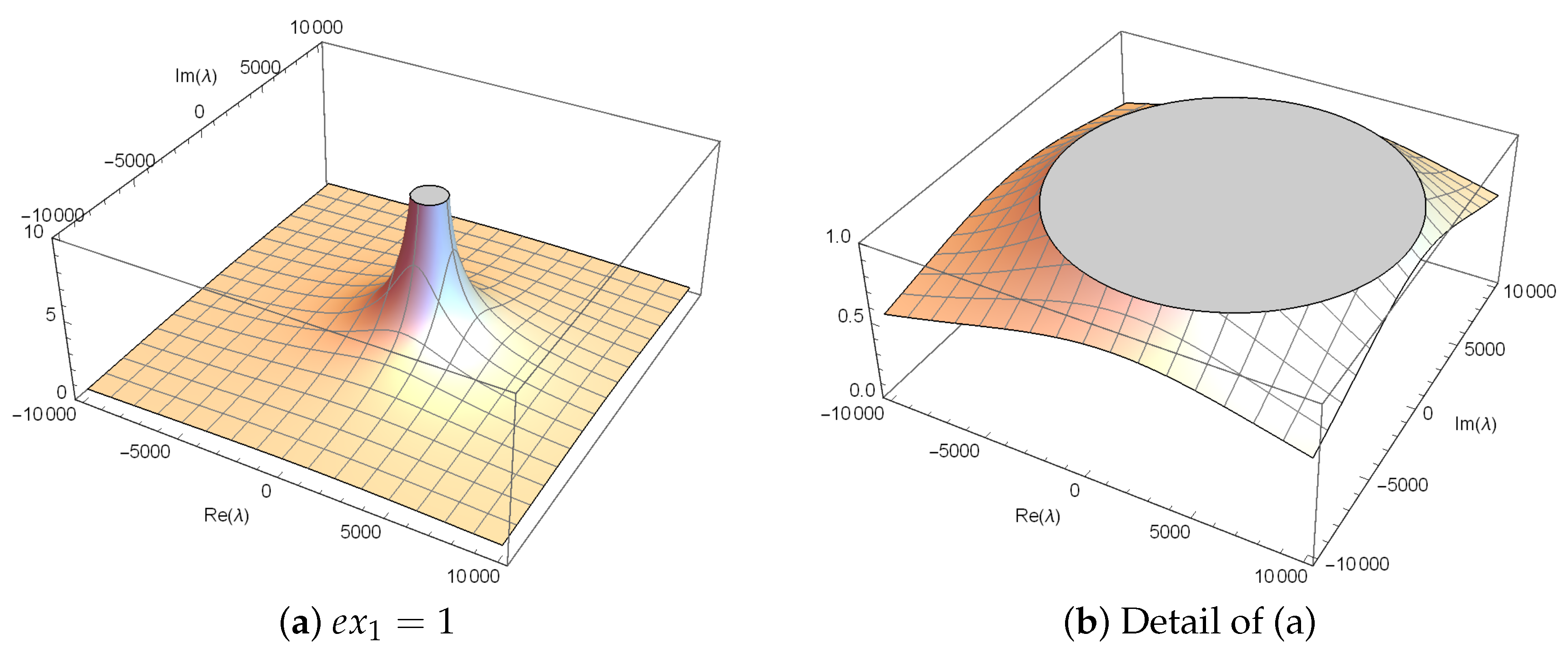
Obviously, no matter what the $\lambda$-value is, 0 and ∞ are superattracting fixed points, while the stability of other fixed points varies with $\lambda \in \mathbb{C}$.

Table 1. Stability of strange fixed points $e{x}_i$ for special $\lambda$-values.

$\mathsf{\lambda }$	${\mathit{ex}}_{\mathit{i}}$			No. of ${\mathit{ex}}_{\mathit{i}}$
	$|{\mathit{R}}_{\mathsf{\lambda }}^{\prime }\left({\mathit{ex}}_{\mathit{i}}\right)|:\mathit{t}$${}^{\mathbf{1}}$
0	$-1.62291\pm 0.455126i$	$-0.611529\pm 1.28544i$	$0.234438\pm 1.48434i$	6
	$6.31492:r$	$4.91253:r$	$7.6094:r$
1344	$-2.57424$	$-0.085032$	$0.123846$	11
	$4.9157:r$	$1.17175\times {10}^{-6}:a$	$6.42351\times {10}^{-6}:a$
	$-2.16337\pm 1.21147i$	$-1.09844\pm 2.04782i$	$0.10715\pm 2.1662i$
	$4.67559:r$	$4.68214:r$	5.53101:r
	$0.922374\pm 1.48996i$
	$5.75625:r$
$-6848$	$-2.81972\pm 0.753267i$	$-1.9133\pm 1.99919i$	$-0.512724\pm 2.5536i$	12
	$4.07847:r$	$3.98574:r$	$4.3251:r$
	$-0.00328839\pm 0.0431351i$	$0.793402\pm 2.17265i$	$1.45563\pm 0.903056i$
	$7.52394\times {10}^{-9}:a$	$4.60277:r$	$3.6229:r$

¹$|R_{\lambda }^{\prime }\left({\mathit{ex}}_i\right)|:t$ implies that ex_i is attractive, parabolic, and repulsive, if $t=a\left(\right|R^{\prime }|<1)$, $t=a\left(\right|R^{\prime }|=1)$, and $t=a\left(\right|R^{\prime }|>1)$, respectively.

summarizes the stability results of strange fixed points $e{x}_i$ corresponding to the special $\lambda$-values related to Proposition 2.

Figure 1 shows the stability surface of $e{x}_1=1$. In Figure 1b, the gray surface represents the repulsion area, while the gold surface represents the attraction area. The attraction area is significantly smaller than the exclusion area. For the $\lambda$-values inside the disk, $e{x}_1$ is a repulsion, while for the $\lambda$-values outside the disk, $e{x}_1$ is an attractor. We are always interested in values within the disk.

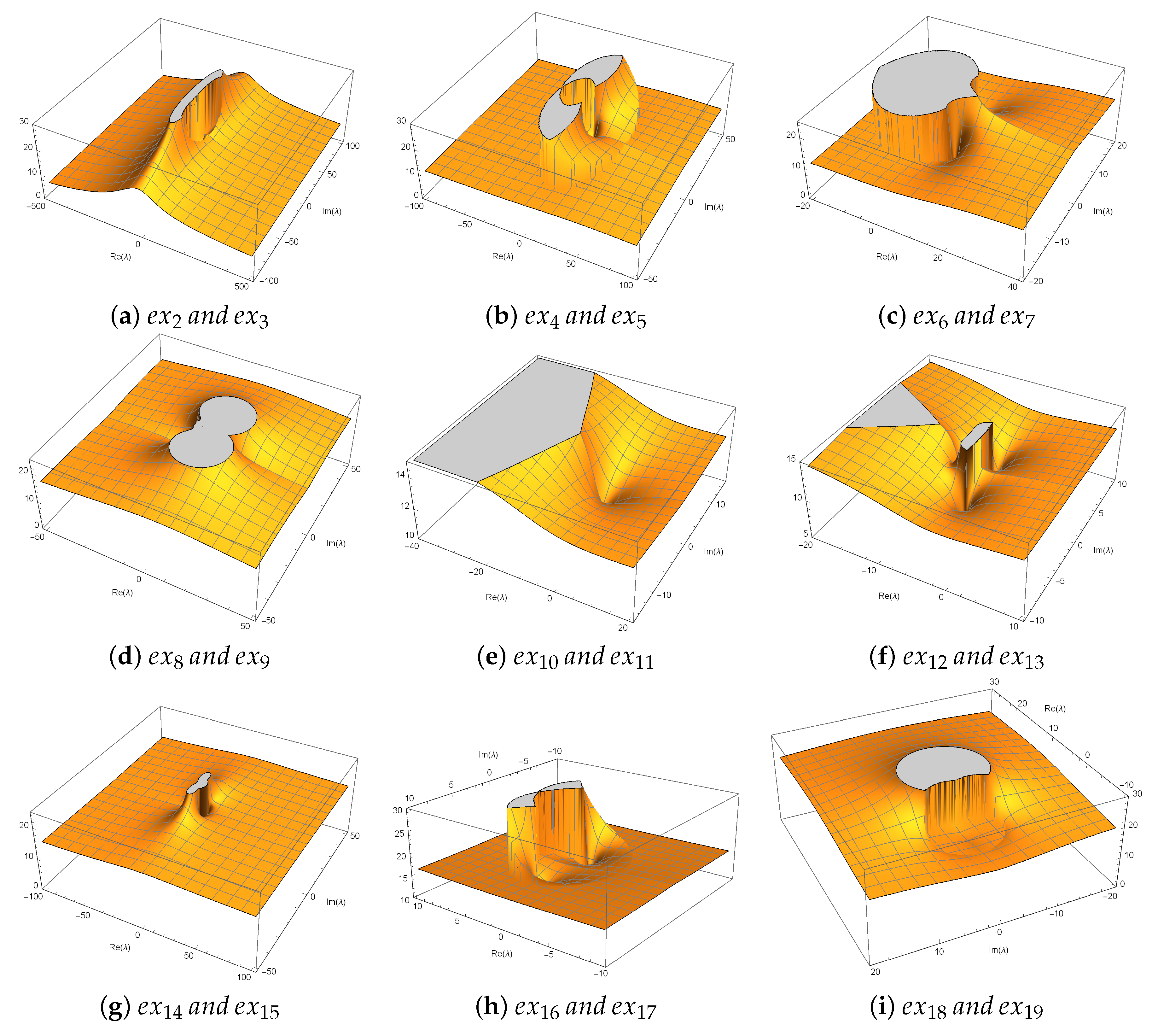
According to Proposition 2, the stability of each pair of conjugate strange fixed points’ representations is the same, so the study of their stability can be reduced from eighteen strange fixed points to nine pairs of strange fixed points. Figure 2 shows the stability surfaces of these nine pairs of strange fixed points. The value of $\lambda$ determines whether these fixed points attract or not. It can be seen from Figure 2 that there are few points that converge to the strange fixed points.

According to (11), the critical points of $R_{\lambda }\left(x\right)$ can be obtained.

Proposition 5.

According to the definition of the critical points, the critical points of $R_{\lambda }\left(x\right)$ are the roots of $R_{\lambda }^{\prime }\left(x\right)=0$, that is to say the process of finding the critical points of $R_{\lambda }\left(x\right)$ is to solve $R_{\lambda }^{\prime }\left(x\right)=0$. That is, $x=0$, $x=\infty$, and the following free critical points:

• $c{r}_1=-1$;
• $c{r}_2=i$;
• $c{r}_3=-i$;
• ${\displaystyle c{r}_4=\frac{1}{2}(-\frac{21}{26}+M\left(\lambda \right)+\frac{1}{2}\sqrt{P\left(\lambda \right)-N\left(\lambda \right)}-\sqrt{{\displaystyle -4+{(\frac{21}{26}-M\left(\lambda \right)-\frac{1}{2}\sqrt{P\left(\lambda \right)-N\left(\lambda \right)})}^2}})}$;
• ${\displaystyle c{r}_5=\frac{1}{2}(-\frac{21}{26}+M\left(\lambda \right)+\frac{1}{2}\sqrt{P\left(\lambda \right)-N\left(\lambda \right)}+\sqrt{{\displaystyle -4+{(\frac{21}{26}-M\left(\lambda \right)-\frac{1}{2}\sqrt{P\left(\lambda \right)-N\left(\lambda \right)})}^2}})}$;
• ${\displaystyle c{r}_6=\frac{1}{2}(-\frac{21}{26}+M\left(\lambda \right)-\frac{1}{2}\sqrt{P\left(\lambda \right)-N\left(\lambda \right)}-\sqrt{{\displaystyle -4+{(\frac{21}{26}-M\left(\lambda \right)+\frac{1}{2}\sqrt{P\left(\lambda \right)-N\left(\lambda \right)})}^2}})}$;
• ${\displaystyle c{r}_7=\frac{1}{2}(-\frac{21}{26}+M\left(\lambda \right)-\frac{1}{2}\sqrt{P\left(\lambda \right)-N\left(\lambda \right)}+\sqrt{{\displaystyle -4+{(\frac{21}{26}-M\left(\lambda \right)+\frac{1}{2}\sqrt{P\left(\lambda \right)-N\left(\lambda \right)})}^2}})}$;
• ${\displaystyle c{r}_8=\frac{1}{2}(-\frac{21}{26}-M\left(\lambda \right)+\frac{1}{2}\sqrt{P\left(\lambda \right)+N\left(\lambda \right)}-\sqrt{{\displaystyle -4+{(\frac{21}{26}+M\left(\lambda \right)-\frac{1}{2}\sqrt{P\left(\lambda \right)+N\left(\lambda \right)})}^2}})}$;
• ${\displaystyle c{r}_9=\frac{1}{2}(-\frac{21}{26}-M\left(\lambda \right)+\frac{1}{2}\sqrt{P\left(\lambda \right)+N\left(\lambda \right)}+\sqrt{{\displaystyle -4+{(\frac{21}{26}+M\left(\lambda \right)-\frac{1}{2}\sqrt{P\left(\lambda \right)+N\left(\lambda \right)})}^2}})}$;
• ${\displaystyle c{r}_{10}=\frac{1}{2}(-\frac{21}{26}-M\left(\lambda \right)-\frac{1}{2}\sqrt{P\left(\lambda \right)+N\left(\lambda \right)}-\sqrt{{\displaystyle -4+{(\frac{21}{26}+M\left(\lambda \right)+\frac{1}{2}\sqrt{P\left(\lambda \right)+N\left(\lambda \right)})}^2}})}$;
• ${\displaystyle c{r}_{11}=\frac{1}{2}(-\frac{21}{26}-M\left(\lambda \right)-\frac{1}{2}\sqrt{P\left(\lambda \right)+N\left(\lambda \right)}+\sqrt{{\displaystyle -4+{(\frac{21}{26}+M\left(\lambda \right)+\frac{1}{2}\sqrt{P\left(\lambda \right)+N\left(\lambda \right)})}^2}})}$;

where:

• ${\displaystyle M\left(\lambda \right)=\frac{1}{2}\sqrt{a\left(\lambda \right)+b\left(\lambda \right)+c\left(\lambda \right)}}$,
• ${\displaystyle P\left(\lambda \right)=\frac{882}{169}+\frac{1}{39}(-128+5\lambda )-b\left(\lambda \right)-c\left(\lambda \right)-N\left(\lambda \right)}$;
• ${\displaystyle N\left(\lambda \right)=\frac{g\left(\lambda \right)}{h\left(\lambda \right)}}$;
• ${\displaystyle a\left(\lambda \right)=\frac{441}{169}+\frac{1}{156}(128-5\lambda )+\frac{1}{52}(-128+5\lambda )}$;
• ${\displaystyle b\left(\lambda \right)=\frac{d\left(\lambda \right)}{156{(e\left(\lambda \right)+18\sqrt{f\left(\lambda \right)})}^{1/3}}}$;
• ${\displaystyle c\left(\lambda \right)=\frac{1}{156}{(e\left(\lambda \right)+18\sqrt{f\left(\lambda \right)})}^{1/3}}$;
• $d\left(\lambda \right)=16384+4696\lambda +25{\lambda }^2$;
• $e\left(\lambda \right)=2097152+1160832\lambda +139578{\lambda }^2-125{\lambda }^3$;
• $f\left(\lambda \right)=3355443200\lambda +2558365696{\lambda }^2+643302144{\lambda }^3+54034441{\lambda }^4-134875{\lambda }^5$;
• ${\displaystyle g\left(\lambda \right)=\frac{74088}{2197}-\frac{42}{169}(128-5\lambda )+\frac{6\lambda }{13}}$;
• $h\left(\lambda \right)=4\sqrt{{\displaystyle \frac{441}{169}+\frac{1}{156}(128-5\lambda )+\frac{1}{52}(-128+5\lambda )+b\left(\lambda \right)+c\left(\lambda \right)}}$.

Choose different λ-values; the number of critical points is also different:

• $R_{\lambda }\left(x\right)$ has 13 critical points, when $\lambda \notin \{0,1344\}$ and $\lambda \in \mathbb{C}$;
• $R_{\lambda }\left(x\right)$ has 7 critical points, when $\lambda =0$;
• $R_{\lambda }\left(x\right)$ has 11 critical points, when $\lambda =1344$;
• The free critical points of $R_{\lambda }\left(x\right)$ satisfy ${\displaystyle c{r}_m=\frac{1}{c{r}_n}}$ for $m\ne n$; each pair is conjugate to each other, being $c{r}_2$ and $c{r}_3$, $c{r}_4$ and $c{r}_5$, $c{r}_6$ and $c{r}_7$, $c{r}_8$ and $c{r}_9$, and $c{r}_{10}$ and $c{r}_{11}$.

Proof. 

From (11), let $R_{\lambda }^{\prime }\left(x\right)=0$:

$${\displaystyle \frac{2x^7{(1+x)}^6{(1+x^2)}^5·{\omega }_{\lambda }\left(x\right)}{{\theta }_{\lambda }{\left(x\right)}^2}=0,}$$

(12)

where ${\omega }_{\lambda }\left(x\right)=52+168x+(336-5\lambda )x^2+3(168+\lambda )x^3+2(284+\lambda )x^4+3(168+\lambda )x^5+(336-5\lambda )x^6+168x^7+52x^8$.

From (12), the free critical points of $R_{\lambda }\left(x\right)$ are $-1,\pm i$ and the eight roots of polynomial ${\omega }_{\lambda }\left(x\right)=0$. Next is the process of solving the expression of the roots of the polynomial ${\omega }_{\lambda }\left(x\right)=0$.

First, we can express ${\omega }_{\lambda }\left(x\right)$ as the product of four quadratic polynomials $(1+d_{i}x+x^2),1\le i\le 4$. We have the following formulas:

$${\omega }_{\lambda }\left(x\right)=52\prod _{i=1}^4(1+d_{i}x+x^2).$$

(13)

Next, by the corresponding coefficients are equal, we can obtain

$$\left\{\begin{array}{c}52(d_1+d_2+d_3+d_4)=168,\\ 52(4+d_1{d}_2+d_1{d}_3+d_2{d}_3+d_1{d}_4+d_2{d}_4+d_3{d}_4)=336-5\lambda ,\\ 52(3d_1+3d_2+3d_3+3d_4+d_1{d}_2{d}_3+d_1{d}_2{d}_4+d_1{d}_3{d}_4+d_2{d}_3{d}_4)=504+3\lambda ,\\ 52(6+2d_1{d}_2+2d_1{d}_3+2d_2{d}_3+2d_1{d}_4+2d_2{d}_4+2d_3{d}_4+d_1{d}_2{d}_3{d}_4)=568+2\lambda .\end{array}\right.$$

(14)

By eliminating $d_2,d_3$, and $d_4$, we can obtain a quartic polynomial about $d_1$:

$$52d_1^4-168d_1^3+(128-5\lambda )d_1^2+3\lambda d_1+12\lambda =0.$$

(15)

After that, the specific expression of $d_i,1\le i\le 4$ can be obtained by (15). Finally, by taking $d_i$ into (13), we can obtain the specific expression of the roots of ${\omega }_{\lambda }\left(x\right)=0$, that is $c{r}_4-c{r}_{11}$.

Additionally,

$${\displaystyle R_0^{\prime }\left(x\right)=\frac{8x^7{(1+x)}^4{(1+x^2)}^3(13+16x+13x^2)}{{(1+4x+9x^2+16x^3+21x^4+20x^5+13x^6)}^2},}$$

(16)

$${\displaystyle R_{1344}^{\prime }\left(x\right)=\frac{8x^7{(1+x)}^6{(1+x^2)}^5(13+68x-1473x^2-1880x^3-1473x^4+68x^5+13x^6)}{{\theta }_{1344}{\left(x\right)}^2},}$$

(17)

where ${\theta }_{1344}\left(x\right)=1+7x+27x^2+77x^3+176x^4+336x^5+552x^6+792x^7+1015x^8+1185x^9-59x^{10}-13x^{11}$.

$${\displaystyle R_{-6848}^{\prime }\left(x\right)=\frac{8x^7{(1+x)}^6{(1+x^2)}^5(13+42x+8644x^2-5010x^3-3282x^4-5010x^5+8644x^6+42x^7+13x^8)}{{\theta }_{-6848}{\left(x\right)}^2},}$$

(18)

where ${\theta }_{-6848}\left(x\right)=1+6x+20x^2+50x^3+99x^4+160x^5+216x^6+240x^7+223x^8+170x^9+6948x^{10}+46x^{11}+13x^{12}$. □

Table 2. Free critical points $c{r}_i$ from $R_{\lambda }^{\prime }\left(c{r}_i\right)$ for special $\lambda$-values.

$\mathsf{\lambda }$	${\mathit{cr}}_{\mathit{i}}$			No. of ${\mathit{cr}}_{\mathit{i}}$
0	$-1$	$\pm i$	$0.615385\pm 0.788227i$	5
1344	$-1$	$\pm i$	$-13.0923$	9
	$-0.0763809$	$0.109819$	$9.10591$
	$-0.638919\pm 0.769274i$
$-6848$	$-1$	$\pm i$	$-1.90256\pm 25.7656i$	11
	$-0.639\pm 0.769207i$	$-0.00285034\pm 0.038601i$	$0.929025\pm 0.370017i$

shows the number of free critical points corresponding to $R_{\lambda }\left(x\right)$, where $\lambda$ is given a particular value. According to the above proposition, 0 and ∞ correspond to the roots of $g\left(x\right)=0$, and the number of free critical points of $R_{\lambda }\left(x\right)$ is at most 11 and at least 5. Since the free critical points $c{r}_1$, $c{r}_2$, and $c{r}_3$ are the pre-images of the strange fixed point $e{x}_1$, the stability of $c{r}_1$, $c{r}_2$, and $c{r}_3$ corresponds to the stability of $e{x}_1$. In addition, as with the strange fixed point in this section, each pair of conjugate free critical points has the same stability properties, so we only need to study the dynamics of half of the free critical points, which will be discussed in Section 2.3.

2.3. Parameter Spaces and Dynamical Planes

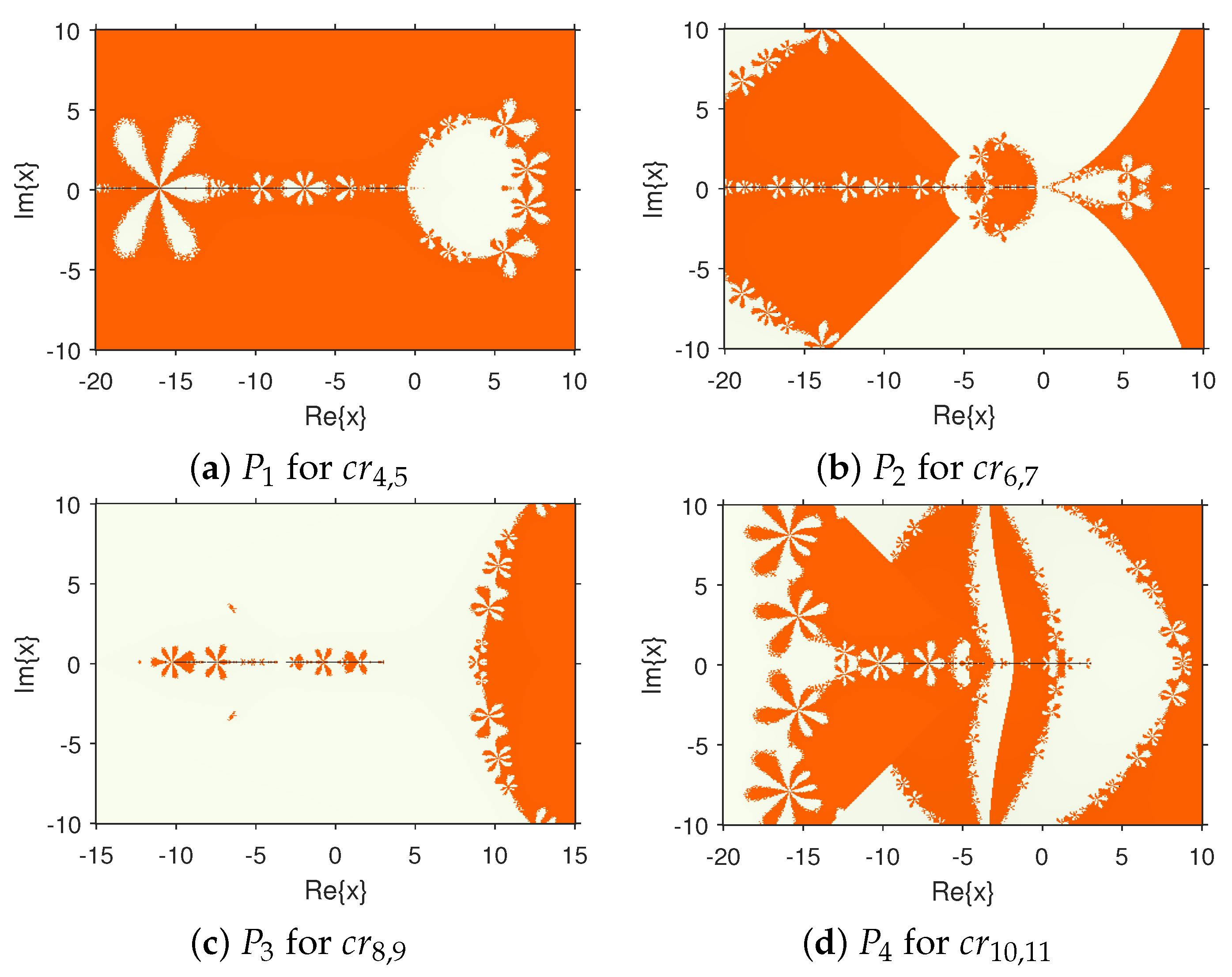
The dynamic behavior of the rational operator $R_{\lambda }\left(x\right)$ (4) varies with the parameter selection. In this section, we discuss the progressive behavior of the free critical points of $LWM\left(\lambda \right)$ through parameter spaces. At first, the parameter space is represented by a $400\times 400$ grid on the complex plane, and the points on the grid correspond to different $\lambda$-values. The parameter space shows the convergence analysis of the $\lambda$-related iterative method (3), where the free critical points $c{r}_i$ in Proposition 5 is used as the initial estimate value and the maximum number of iterations is 25. If it converges to 0, it is expressed as orange. If it converges to ∞, it is expressed as faint yellow, and other cases are expressed as black.

Our goal was to find a relatively stable region in the parameter space, that is the orange and faint yellow regions, because the $\lambda$-values in these regions are the best parameter members in terms of numerical stability.

The $LWM\left(\lambda \right)$ family has a maximum of eleven free critical points. Proposition 5 states that it is sufficient to study four different parameter spaces. These parameter spaces are called $P_1(forx=c{r}_4,c{r}_5)$, $P_2(forx=c{r}_6,c{r}_7)$, $P_3(forx=c{r}_8,c{r}_9)$, and $P_4(forx=c{r}_{10},c{r}_{11})$, as described in Figure 3. Among them, the large area of Figure 3 is orange and faint yellow, that is, in most cases, it converges to the roots. However, by carefully observing the details of the parameter spaces, we can see that the rare black area near the imaginary part of the parameter $\lambda$ is 0. For example, the points corresponding to $\lambda =-7$, $\lambda =-11.68$, $\beta =-9.69$, and $\beta =-4.999$ in $P_1$–$P_4$ are in the black regions. Combining Figure 1 and Figure 2, we know that only a quite small part of the points in the iterative method (3) converge to the strange fixed points, which corresponds to the results shown in $P_1$–$P_4$, indicating that the members in $LWM\left(\lambda \right)$ are numerically stable.

Then, we explored the stability of the corresponding iterative method by selecting various parameter values to generate a dynamical plane.

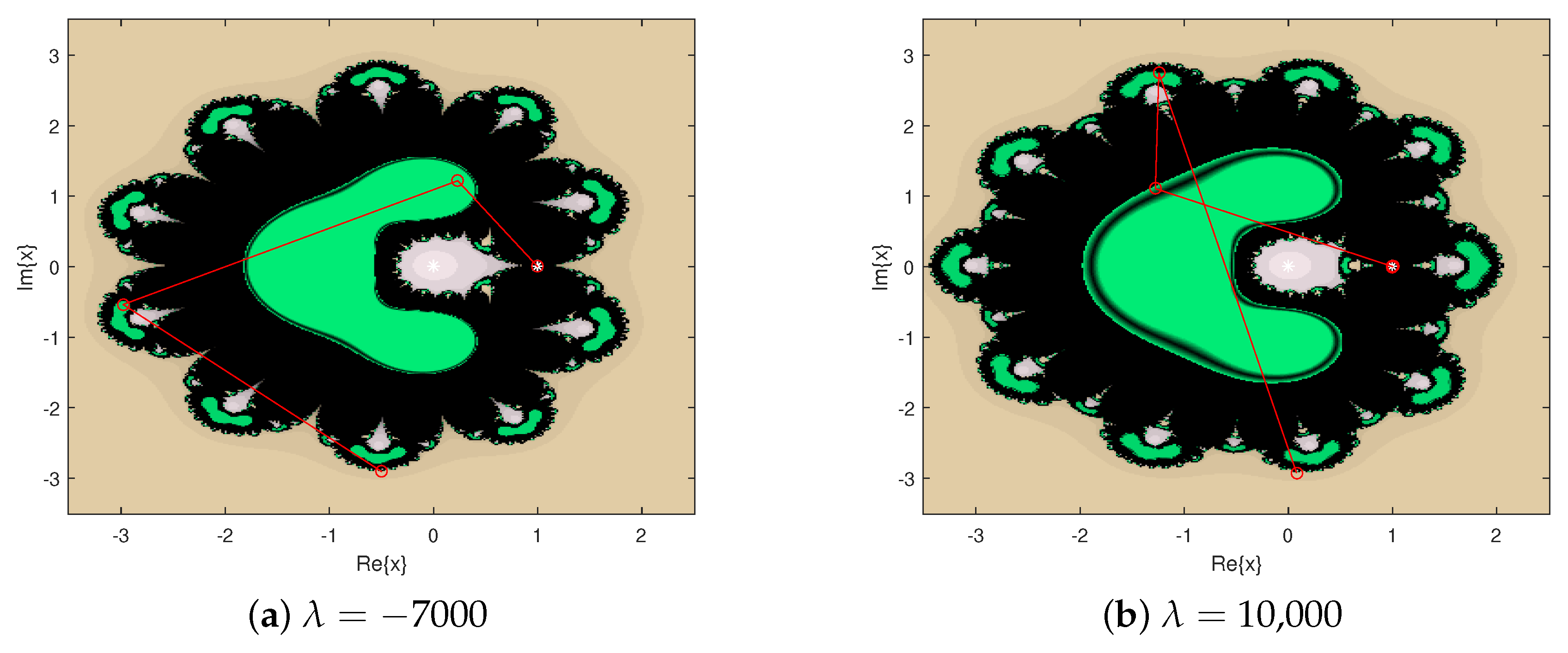
Firstly, a grid generated by $400\times 400$ points is defined on the complex plane, where each point on the grid corresponds to a different value of the initial estimate $x_0$. Its graphical representation indicates that this method has a maximum of 25 iterations to any root starting from $x_0$. Among them, the white asterisk “∗” represents the attractive point. Fixed points are illustrated with a red circle “∘”. Periodic points are represented as blue squares “⋄”. In addition, we represent the orbit of a periodic point in blue and the orbit of a fixed point in red.

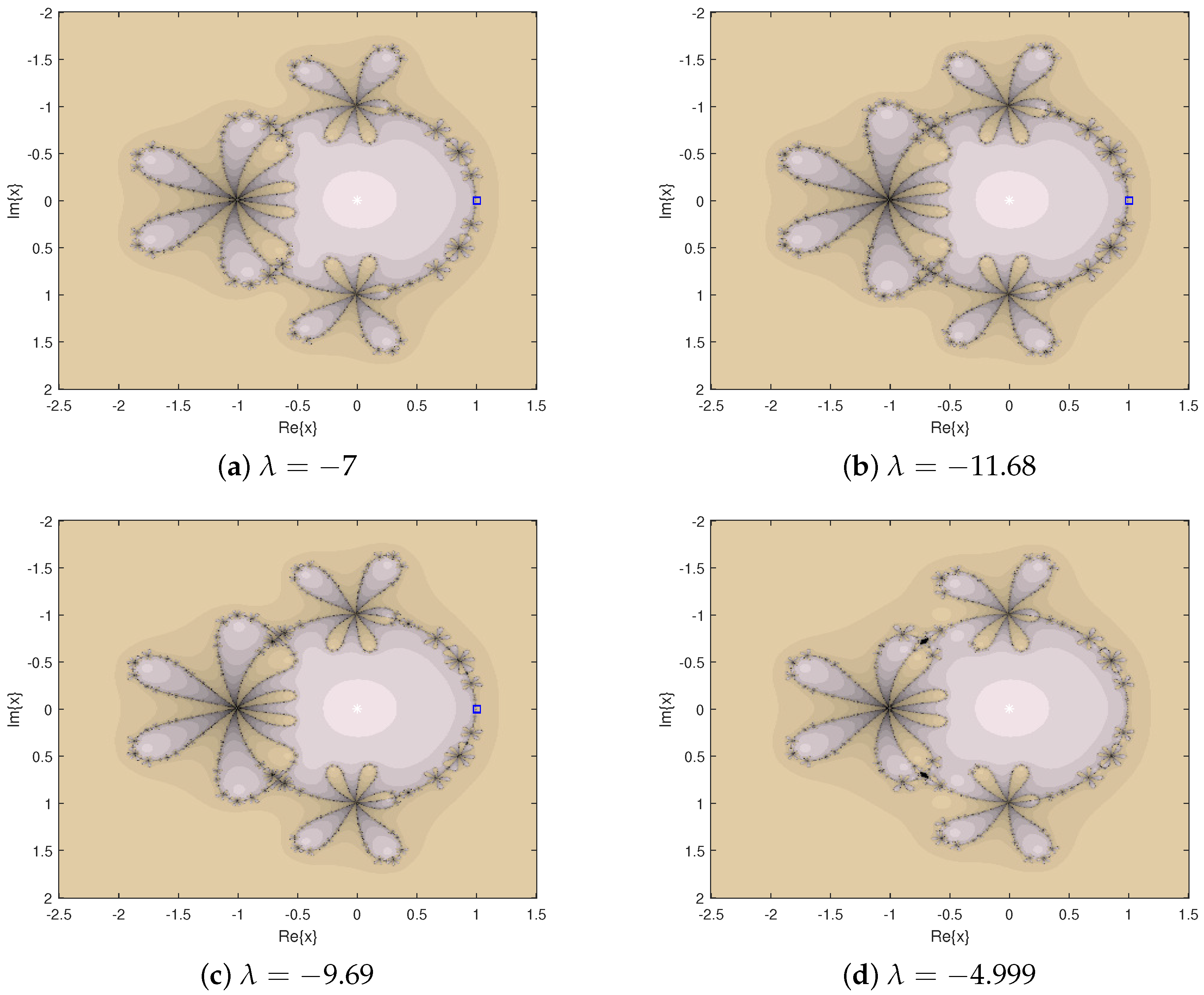
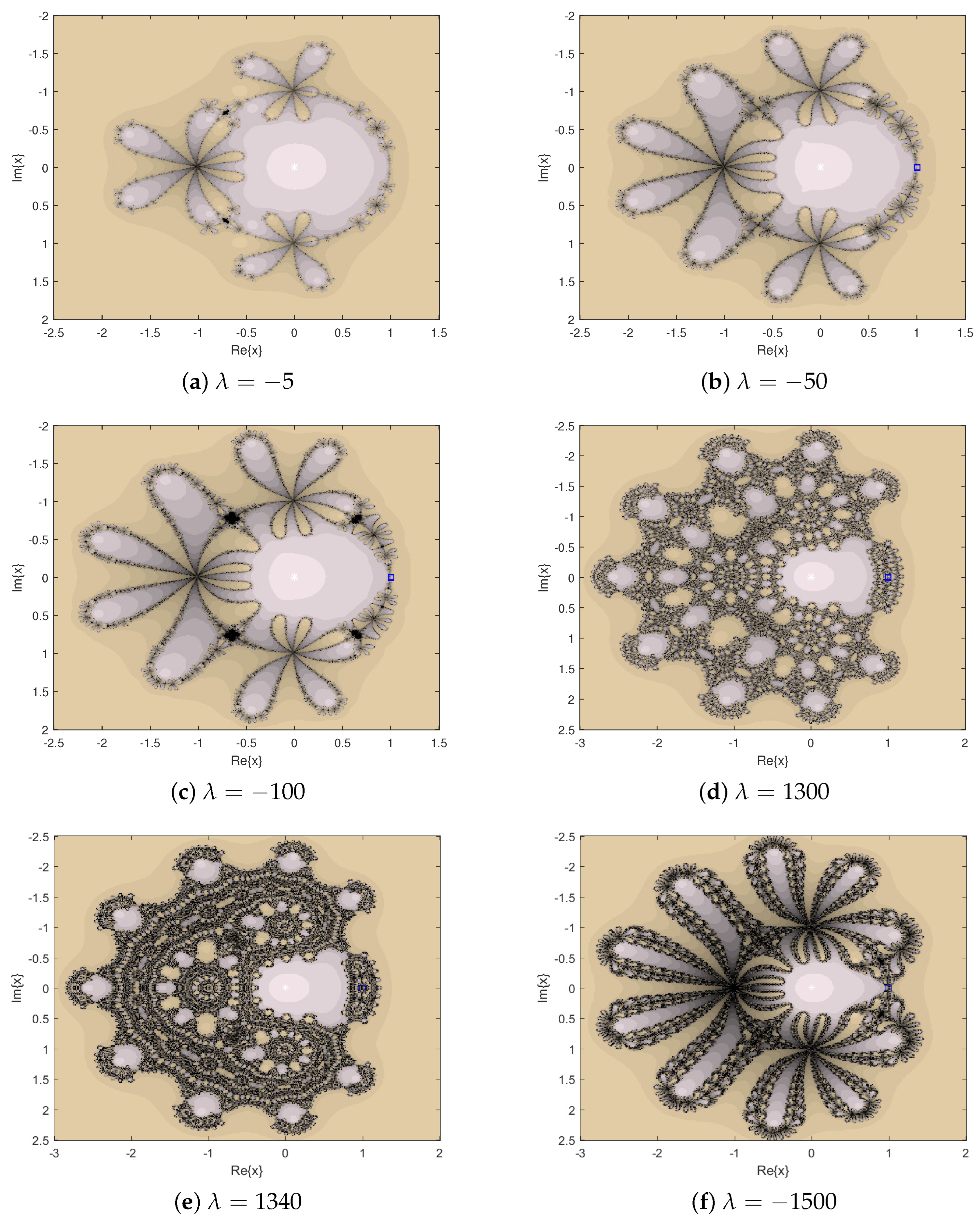
Figure 4, Figure 5, Figure 6 and Figure 7 show the dynamical planes of $LWM\left(\lambda \right)$ corresponding to a given $\lambda$ value. Different colors represent different basins of attraction: gray represents convergence to 0, khaki convergence to ∞, green convergence to fixed point $e{x}_1=1$, and black non-convergence.

Next, the stability of some $LWM\left(\lambda \right)$ was studied by generating a dynamical plane. We discuss the choice of parameter $\lambda$ in four parts. In the first part, we chose the parameter values in the black regions of the parameter spaces, that is $\lambda =-7,-11.68,-9.69,-4.999$; see Figure 4.

In the second part, we selected the parameter values that satisfy $|\lambda -1344|<8192$, which is divided into two parts: one is the smaller value, $\lambda =-5,-50,-100$, and the other part is the larger value, $\lambda =1300,1340,-1500$. At this time, $e{x}_1=1$ is the attractive point, which corresponds to the conclusion of Proposition 4$\left(b\right)$; see Figure 5.

In the third part, we drew $\lambda =-7000,$ 10,000, which correspond to the conclusion of the proposition in Figure 4a; see Figure 6.

Finally, we drew the dynamical plane of $\lambda =0,-6848,1344$, where $\lambda$ are the special values obtained in Proposition 2; see Figure 7.

In Figure 4, Figure 5, Figure 6 and Figure 7, the dynamical planes of most parameters converge to 0 and ∞, but there are also parameter values that make the iterative method not converge, such as the parameter $\lambda =-4.999$ in Figure 4 and $\lambda =-5,-100$ in Figure 5. Note from Figure 6 that the iterative method corresponding to the parameters satisfying $|\lambda -1344|>8192$ converges to two extra fixed points in addition to $0,\infty ,e{x}_1=1$. This indicates that the iterative method corresponding to these parameters is unstable. What we want to study more is stable parameters, that is the dynamical planes only show gray and khaki.

Comparing Figure 4, Figure 5, and Figure 7, we can see that the larger the absolute value of the parameter values, the more complex the dynamical plane displayed. Carefully observing the black area in Figure 4d and Figure 5a,c, we can also observe that the larger the absolute value of the parameter values, the larger the black area is. In summary, the iterative method corresponding to $\lambda =0$ is more stable.

3. Numerical Experiment and Practical Application

In this section, the more stable parameter elements obtained in Section 2, namely $\{0,-50,1300,1340,-1500\}$, are verified by a numerical experiment and applied to solve practical problem.

First, we used the iterative method corresponding to these parameters to solve the nonlinear matrix sign function:

$$X^2-I=0,Iisanidentitymatrix.$$

After that, we obtained the following special cases:

• When $\lambda =0$, $X_{n+1}=128X_n^5{(I+X_n^2)}^4{[I-9X_n^2+57X_n^4+247X_n^6+763X_n^8+637X_n^{10}+331X_n^{12}+21X_n^{14}]}^{-1}$;
• When $\lambda =-50$, $X_{n+1}=8192X_n^7{(I+X_n^2)}^6{[50{(-I+X_n^2)}^{10}+64{(X_n+X_n^3)}^2(I-9X_n^2+57X_n^4+247X_n^6+763X_n^8+637X_n^{10}+331X_n^{12}+21X_n^{14})]}^{-1}$;
• When $\lambda =1300$, $X_{n+1}=8192X_n^7{(I+X_n^2)}^6{[-1300{(-I+X_n^2)}^{10}+64{(X_n+X_n^3)}^2(I-9X_n^2+57X_n^4+247X_n^6+763X_n^8+637X_n^{10}+331X_n^{12}+21X_n^{14})]}^{-1}$;
• When $\lambda =1340$, $X_{n+1}=8192X_n^7{(I+X_n^2)}^6{[-1340{(-I+X_n^2)}^{10}+64{(X_n+X_n^3)}^2(I-9X_n^2+57X_n^4+247X_n^6+763X_n^8+637X_n^{10}+331X_n^{12}+21X_n^{14})]}^{-1}$;
• When $\lambda =-1500$, $X_{n+1}=8192X_n^7{(I+X_n^2)}^6{[1500{(-I+X_n^2)}^{10}+64{(X_n+X_n^3)}^2(I-9X_n^2+57X_n^4+247X_n^6+763X_n^8+637X_n^{10}+331X_n^{12}+21X_n^{14})]}^{-1}$.

Finally, we used the Matlab software to record the iteration times and computer running time of the experimental results of solving the matrix symbol function corresponding to the random square matrix. The calculation stopping standard is $\Vert X_n^2{-I\Vert }_2\le {10}^{-100}$. The experimental results are shown in

Table 3. Results of the comparisons.

	$\mathsf{\lambda }=0$		$\mathsf{\lambda }=-50$		$\mathsf{\lambda }=1300$		$\mathsf{\lambda }=1340$		$\mathsf{\lambda }=-1500$
Matrices	n${}^1$	Time	n	Time	n	Time	n	Time	n	Time
$R_{4\times 4}$	3	$0.006994$	5	$0.079566$	6	$0.074327$	6	$0.103540$	5	$0.108107$
$R_{5\times 5}$	3	$0.016522$	13	$0.066437$	13	$0.094517$	9	$0.122004$	16	$0.129702$
$R_{10\times 10}$	5	$0.069684$	10	$0.139051$	27	$0.136659$	41	$0.157447$	15	$0.059954$
$R_{15\times 15}$	6	$0.070848$	21	$0.160829$	22	$0.187887$	13	$0.158099$	86	$0.279862$
$R_{20\times 20}$	6	$0.071416$	19	$0.180107$	19	$0.186666$	17	$0.162618$	103	$0.718463$
$R_{25\times 25}$	9	$0.111521$	14	$0.143166$	20	$0.209045$	13	$0.158114$	97	$0.380726$
$R_{30\times 30}$	8	$0.136161$	28	$0.203730$	16	$0.177654$	15	$0.176462$	191	$0.832457$

¹n represents the number of iterations.

.

Through the results in Table 3, we noticed that, in $\{0,-50,1300,1340,-1500\}$, when $\lambda =0$, the iterative method (3) is used to solve the matrix function with the least number of iterations and the shortest computer running time.

In 1873, van der Waals revised the equation of state of the ideal gas and proposed the van der Waals equation of state based on the two assumptions of the ideal gas model, namely the non-occupying volume of molecules and the non-interacting force between molecules. The volume occupied by molecules decreases their free space of movement, and the frequency of molecules hitting the container wall increases at the same temperature, so the pressure increases correspondingly. If $V_m-b$ is used to represent the free movement space per mole of gas molecules, the gas pressure should be $P=RT/(V_m-b)$ by referring to the ideal gas equation of state.

The specific form of Van der Waals equation is:

$${\displaystyle (P+a\frac{n^2}{V^2})(V-nb)=nRT}$$

where a and b are the relative constants corrected for gas pressure and volume, respectively, which are called the van der Waals constants. Each gas has a specific value for a and b. $n,R,T,V$, and P represent the number of moles, the universal gas constant (0.0820578), the absolute temperature, the volume, and the absolute pressure, respectively.

By simplification, the following polynomial of the nonlinear form can be obtained:

$$H\left(V\right)=P{V}^3-(RT+bP)V^{2}n+aV{n}^2-ab{n}^3.$$

When $n=1.5$ moles of benzene vapor, $P=50atm$, $a=1.378$, and $b=0.3193$, then there is

$$H_1\left(V\right)=50V^3-119.0185191V^2+3.1005V-1.484984475.$$

The exact solution to $H_1\left(V\right)=0$ is

$V=2.3594236086921194141576714329391903003579204650023$

(50 significant digits).

Next, we used the iterative method (3) with $\lambda =0$ and the other three eighth-order iterative methods to solve $H_1\left(V\right)=0$ and compared the results. According to Theorem 1 in [21], when applying the iterative method $LWM$ (3) to solve nonlinear equations, in order to maintain the convergence rate of the eighth order, we must select the initial point near the exact solution, so that the initial point is close enough to the exact solution. Therefore, we chose the initial estimate of $x_0=2.36$. The experimental results are shown in

Table 4. Comparison of iterative methods for $H_1\left(V\right)=0$.

n	$\mathit{LWM}$		$\mathit{SM}$		$\mathit{SSM}$
	$\mathbf{|}{\mathit{x}}_{\mathit{n}}\mathbf{-}{\mathit{x}}_{\mathit{n}\mathbf{-}\mathbf{1}}\mathbf{|}$	$\mathbf{\left|}\mathit{f}\mathbf{\right(}{\mathit{x}}_{\mathit{n}}\mathbf{\left)}\mathbf{\right|}$	$\mathbf{|}{\mathit{x}}_{\mathit{n}}\mathbf{-}{\mathit{x}}_{\mathit{n}\mathbf{-}\mathit{1}}\mathbf{|}$	$\mathbf{\left|}\mathit{f}\mathbf{\right(}{\mathit{x}}_{\mathit{n}}\mathbf{\left)}\mathbf{\right|}$	$\mathbf{|}{\mathit{x}}_{\mathit{n}}\mathbf{-}{\mathit{x}}_{\mathit{n}\mathbf{-}\mathbf{1}}\mathbf{|}$	$\mathbf{\left|}\mathit{f}\mathbf{\right(}{\mathit{x}}_{\mathit{n}}\mathbf{\left)}\mathbf{\right|}$
1	$5.7639\times {10}^{-4}$	$1.818\times {10}^{-21}$	$1.1528\times {10}^{-3}$	$1.593\times {10}^{-1}$	$5.7639\times {10}^{-4}$	$1.4902\times {10}^{-19}$
2	$6.5748\times {10}^{-24}$	$4.1048\times {10}^{-47}$	$1.1528\times {10}^{-3}$	$1.5945\times {10}^{-1}$	$5.3893\times {10}^{-22}$	$1.6823\times {10}^{-45}$
3	$1.4846\times {10}^{-49}$	$9.2685\times {10}^{-73}$	$1.1528\times {10}^{-3}$	$1.593\times {10}^{-1}$	$6.0843\times {10}^{-48}$	$1.8993\times {10}^{-71}$
4	$3.352\times {10}^{-75}$	$2.0928\times {10}^{-98}$	$1.1528\times {10}^{-3}$	$1.5945\times {10}^{-1}$	$6.869\times {10}^{-74}$	$2.1442\times {10}^{-97}$

.

The method by Sharma et al., $SM$ (see [25]), is

$$\left\{\begin{array}{c}{\displaystyle w_n=x_n-\frac{f\left(x_n\right)}{f^{\prime }\left(x_n\right)},}\\ {\displaystyle z_n=w_n-\frac{f\left(w_n\right)}{f^{\prime }\left(x_n\right)}\frac{f\left(x_n\right)+af\left(w_n\right)}{f\left(x_n\right)+(a-2)f\left(w_n\right)},}\\ {\displaystyle x_{n+1}=x_n-\frac{P+Q+R}{Pf[z_n,x_n]+Q{f}^{\prime }\left(x_n\right)+Rf[w_n,x_n]}f\left(x_n\right).}\end{array}\right.$$

(19)

where $P=(x_n-w_n)f\left(x_n\right)f\left(w_n\right)$, $Q=(w_n-z_n)f\left(w_n\right)f\left(z_n\right)$ and $R=(z_n-x_n)f\left(z_n\right)f\left(x_n\right)$. We chose $a=0$ for the numerical experiment part.

The method by Soleymani, $SSM$ (see [26]), is

$$\left\{\begin{array}{c}{\displaystyle y_n=x_n-\frac{f\left(x_n\right)}{f^{\prime }\left(x_n\right)},}\\ {\displaystyle z_n=y_n-\frac{f\left(y_n\right)}{f^{\prime }\left(x_n\right)}\frac{f\left(x_n\right)+\beta f\left(y_n\right)}{f\left(x_n\right)+(\beta -2)f\left(y_n\right)},}\\ {\displaystyle x_{n+1}=z_n-\frac{f\left(z_n\right)}{f^{\prime }\left(x_n\right)}\left\{\frac{f\left(x_n\right)+\beta f\left(y_n\right)}{f\left(x_n\right)+(\beta -2)f\left(y_n\right)}\right\}(1+2t+\mu +{\mu }^2+{\rho }^2+4{\rho }^3+12{\rho }^4-\sigma -{\tau }^2).}\end{array}\right.$$

(20)

where ${\displaystyle t=\frac{f\left(z_n\right)}{f\left(x_n\right)},\mu =\frac{f\left(z_n\right)}{f\left(y_n\right)},\rho =\frac{f\left(y_n\right)}{f\left(x_n\right)},\sigma =\frac{f\left(z_n\right)}{f^{\prime }\left(x_n\right)}}$, and ${\displaystyle \tau =\frac{f\left(y_n\right)}{f^{\prime }\left(x_n\right)}}$. We chose $\beta =0$ for the numerical experiment part.

It can be seen from the experimental results in Table 4 that the $LWM$ with $\lambda =0$ is more dominant in convergence accuracy.

4. Conclusions

In this paper, as stated by fractal theory, we explored the complex dynamic behavior of a kind of iterative method (3) for solving nonlinear equations. Among them, Liu–Wang’s method is based on the well-known Ostrowski method, which adds a step to make it the optimal eighth-order iterative method with faster convergence speed.

Based on the theory of the Möbius conjugate transformation on the Riemann sphere and the scaling theorem, we obtained the corresponding rational operator by applying any quadratic polynomial to the iterative method. The operator can be simplified by giving parameters to facilitate the subsequent research. First, we analyzed its fixed points and the critical points and noticed that the strange fixed points always appeared in pairs, because the two strange points were conjugate, as were the free critical points. Given this relationship, then the number of studies on them could be reduced by half. All of this was performed with the Mathematica software. By drawing the stability surfaces of the strange fixed points, we can observe the range of parameters that can attract the sequence generated by the initial point to the strange fixed point during the iteration. Since we expected that these sequences can converge to the roots rather than the strange fixed points. Based on the above parameter range, we can more effectively select the desired parameters and avoid selecting bad parameters. What is more, the parameter space generated by the iteration with the critical point as the initial point was drawn, so as to obtain a stable parameter selection region. Combining the dynamical planes’ analysis of the given parameters, we finally obtained some parameter families that made the iterative method stable, such as $\lambda =0,-50,1300,1340,-1500$. When these parameters were selected, the corresponding iterative method had good numerical stability, especially at $\lambda =0$. Finally, this result was proven by solving the matrix sign function and the van der Waals equation.

References

- Sidorov, N. Special Issue Editorial “Solvability of Nonlinear Equations with Parameters: Branching, Regularization, Group Symmetry and Solutions Blow-Up”. Symmetry 2022, 14, 226. [Google Scholar] [CrossRef]
- Hassan, M.; Muhammed, A.A. Globally convergent diagonal Polak-Ribière-Polyak like algorithm for nonlinear equations. Numer. Algorithms 2022, 91, 1441–1460. [Google Scholar]
- Wang, X.; Chen, X. Derivative-Free Kurchatov-Type Accelerating Iterative Method for Solving Nonlinear Systems: Dynamics and Applications. Fractal Fract. 2022, 6, 59. [Google Scholar] [CrossRef]
- Geum, Y.H.; Kim, Y.I.; Magreñán, Á.A. A biparametric extension of King’s fourth-order methods and their dynamics. Appl. Math. Comput. 2016, 282, 254–275. [Google Scholar] [CrossRef]
- Nilay, K.R. A new semi-explicit atomistic molecular dynamics simulation method for membrane proteins. J. Comput. Methods Sci. Eng. 2019, 19, 259–286. [Google Scholar]
- Zhang, Z.; Choon, C.F.; Liu, G.R. A Semi-Explicit Finite Element Method for Dynamic Analysis of Dielectric Elastomers. Int. J. Comp. Meth-sing. 2015, 12, 1350108. [Google Scholar] [CrossRef]
- Zhao, X.; Liu, M.; Wang, P.; Guan, J.; Wang, X. Highly efficient preparation of multi-angle continuous carbon fibre reinforced hydroxyapatite composites by electrostatic splitting method. J. Eur. Ceram. Soc. 2022, 42, 7631–7647. [Google Scholar] [CrossRef]
- Dong, Y. A new splitting method for systems of monotone inclusions in Hilbert spaces. Math. Comput. Simulat. 2023, 203, 518–537. [Google Scholar] [CrossRef]
- Dai, L.; Singh, M.C. An analytical and numerical method for solving linear and nonlinear vibration problems. Int. J. Solids Struct. 1997, 34, 2709–2731. [Google Scholar] [CrossRef]
- Cordero, A.; Torregrosa, J.R.; Vassileva, M.P. Three-step iterative methods with optimal eighth-order convergence. J. Comput. Appl. Math. 2011, 235, 3189–3194. [Google Scholar] [CrossRef] [Green Version]
- Cordero, A.; Moscoso-Martínez, M.; Torregrosa, J.R. Chaos and Stability in a New Iterative Family for Solving Nonlinear Equations. Algorithms 2021, 14, 101. [Google Scholar] [CrossRef]
- Cordero, A.; Leonardo, S.M.A.; Torregrosa, J.R. Dynamics and Stability on a Family of Optimal Fourth-Order Iterative Methods. Algorithms 2022, 15, 387. [Google Scholar] [CrossRef]
- Kanwar, V.; Bhatia, S.; Kansal, M. New optimal class of higher-order methods for multiple roots. College Math. J. 2013, 222, 564–574. [Google Scholar]
- Wang, X.; Zhang, T.; Qin, Y. Efficient two-step derivative-free iterative methods with memory and their dynamics. Int. J. Comput. Math. 2016, 93, 1423–1446. [Google Scholar] [CrossRef]
- Ortega, J.M.; Rheinbolt, W.C. Iterative Solution of Nonlinear Equations in Several Variables; Academic Press: New York, NY, USA, 1970. [Google Scholar]
- Kou, J.; Li, Y.; Wang, X. Modified Halley’s method free from second derivative. Appl. Math. Comput. 2006, 183, 704–708. [Google Scholar] [CrossRef]
- Neta, B. On Popovski’s method for nonlinear equations. Appl. Math. Comput. 2008, 201, 710–715. [Google Scholar] [CrossRef] [Green Version]
- Kung, H.T.; Traub, J.F. Optimal order of one-point and multipoint iteration. J. Assoc. Comput. Mach. 1974, 21, 634–651. [Google Scholar] [CrossRef]
- Husain, A.; Nanda, M.N.; Chowdary, M.S.; Sajid, M. Fractals: An Eclectic Survey, Part-I. Fractal Fract. 2022, 6, 89. [Google Scholar] [CrossRef]
- Husain, A.; Nanda, M.N.; Chowdary, M.S.; Sajid, M. Fractals: An Eclectic Survey, Part II. Fractal Fract. 2022, 6, 379. [Google Scholar] [CrossRef]
- Liu, L.; Xia, W. Eighth-order methods with high efficiency index for solving nonlinear equations. Appl. Math. Comput. 2010, 215, 3449–3454. [Google Scholar] [CrossRef]
- Lee, M.Y.; Kim, Y.I. The dynamical analysis of a uniparametric family of three-point optimal eighth-order multiple-root finders under the Möbius conjugacy map on the Riemann sphere. Numer. Algorithms 2020, 83, 1063–1090. [Google Scholar] [CrossRef]
- Wang, X.; Li, W. Choosing the Best Members of the Optimal Eighth-Order Petković’s Family by Its Fractal Behavior. Fractal Fract. 2022, 6, 749. [Google Scholar] [CrossRef]
- Amat, S.; Busquier, S.; Plaza, S. Chaotic dynamics of a third-order Newton-type method. J. Math. Anal. Appl. 2010, 366, 24–32. [Google Scholar] [CrossRef] [Green Version]
- Sharma, J.R.; Guha, R.K.; Gupta, P. Improved King’s methods with optimal order of convergence based on rational approximations. Appl. Math. Lett. 2013, 26, 473–480. [Google Scholar] [CrossRef]
- Soleymani, F.; Vanani, S.K.; Khan, M.; Sharifi, M. Some modifications of King’s family with optimal eighth order of convergence. Math. Comput. Model. 2012, 55, 1373–1380. [Google Scholar] [CrossRef]
Figure 1.
Stability surface of .
Figure 2.
Stability surfaces of other strange fixed points.
Figure 3.
Parameter spaces .
Figure 4.
Dynamical planes for special -values.
Figure 5.
Figure 6.
Figure 7.