1. Introduction
Kaufmann and Tödtling (2001) emphasized that firms should develop scientific technologies to launch innovative products in the market [
1]. At present, firms are actively reflecting technologies in their management plans. They employ technologies to (
i) pinpoint their strengths [
2,
3,
4], (
ii) compare them with those of competitors [
5,
6,
7], and (
iii) develop new business models [
8,
9]. Furthermore, firms create intellectual property (IP) from their management activities based on their technology, which comprises the IP research and development (IP-R&D) of firms.
Generally, IP-R&D employs patents, which are typical IPs. Firms can claim their rights to specific technologies, such as patents. Thus, firms proactively use patents for prior arts, prediction of emerging technology, and technology evaluations. These patents explain (i) how novel technology is, (ii) how advanced technology is compared to prior art, and (iii) how technology contributes to industrial development. Patents can also explain the features of technologies such as originality, marketability, and scope of rights using various factors.
Patents include citations, family patents, and claims. Citations refer to the number of cited papers of prior art or cited information by other patents. The originality of technology can be measured based on the citations of the patent [
10,
11,
12]. As firms want their technologies to be widely used, they register patent families in a number of nations. Therefore, patent families can be used as factors to estimate the marketability of the technology [
13]. Claims refer to the scope of rights of the technology. The higher the number of claims is, the wider the scope of rights to protect the patent [
14,
15].
IP-R&D using patent factors has been studied in various forms. Firms have several IP-R&D strategies that can be used to develop innovative products and services. First, firms can reduce the cost of R&D through technology trade or transfer [
16,
17]. Second, the prediction of vacant technology can help the discovery of new business models for firms [
18]. Third, firms can predict emerging technology to invest in their limited budgets efficiently and intensively [
19]. Finally, technology evaluation can be used in the planning of various IP-R&D activities such as the prediction of technology transfer, vacant technology, and emerging technology [
20,
21].
IP-R&D can also help predict the future of technology through various factors of patents. These advantages act as a sufficient condition for industry, academia, and even the government to select IP-R&D. However, we need to consider the uncertainty of patent factors to establish more complete IP-R&D strategies. This is because the basis of IP-R&D is trust in factors that explain the features of technology.
The purpose of this study is to estimate the uncertainty of various patent factors used in IP-R&D. In particular, we focus on technology evaluation for the following reasons.
Technology evaluation that can predict technology excellence is a bridge that connects various types of IP-R&D and firms.
The technology value may fluctuate depending on the time of evaluation.
The uncertainty of technology value can be actively reflected in the management and investment of firms.
Thus, we estimate the uncertainty of factors used in technology evaluation in order to (i) help firms make the right decisions, (ii) support timely R&D, and (iii) contribute towards minimizing losses. To achieve this, this study proposes a Bayesian neural network (BNN) model for technology evaluation. The proposed methodology not only estimates the uncertainty of evaluation factors but also predicts the patent value.
The contributions of the proposed methodology are as follows:
Jun (2022) and Uhm and Jun (2022) pointed out the intractable limitations of the Bayesian approach as the volume of big data gradually increased [
22,
23]. To improve these limitations, we applied Flipout as a tractable and appropriate approach to big data. Flipout helped BNN learn each layer independently.
Lee and Park (2022) emphasized that identifying factors influencing IP-R&D can prevent the absence of validity in patent analysis [
24]. Thus, we measured the influence on the technology value for each evaluation factor. To this end, the difference between the mean and variance of the value according to the factor was statistically tested.
Choi et al. (2023) argued that for sustainable growth in an uncertain business environment, it is necessary to cope with the rapidly changing flow of technology [
25]. Therefore, we measured the uncertainty of technology evaluation over time. In addition, we verified the trend and presented empirical evidence for the timeliness and objectivity of technology evaluation.
The rest of the paper is structured as follows.
Section 2 and
Section 3 explain the previous studies on technology evaluation and the background of the Bayesian neural network, respectively.
Section 4 proposes a method for estimating technology evaluation factors.
Section 5 describes an experiment to demonstrate the applicability of our method. Finally,
Section 6 discusses several limitations of our study, and
Section 7 presents suggestions for future studies.
2. Related Works
In the past, technology evaluations were conducted based on the opinions of technology experts. However, as patent data increase and computing power improves, a large number of studies on social network analysis or the use of machine learning and deep learning have been conducted.
Previously, technology evaluation has been conducted via the expert-based Delphi method [
26,
27]. However, such methodologies potentially produced biased evaluations depending on the opinion of individual experts. Furthermore, they did not reflect various factors included in patents and could not predict the future technology value. To overcome these limitations, Galbraith et al. (2006) proposed a combination of technology evaluation factors and an expert-based method [
28]. Furthermore, Akoka and Comyn-Wattiau (2017) pointed out the risk of evaluation of new technologies and stressed the need for a methodology that can reflect this risk [
29]. Sa et al. (2022) suggested a Delphi-based methodology, noting that the opinions of experts and academics are important to capturing and evaluating the value of technology [
30].
Patents cite prior art to protect rights and technological progress. Owing to this characteristic, several researchers analyzed patents using a form of a social network. Kim et al. (2015) used connected patent information in a network to evaluate the excellence of technology [
31]. Choi et al. (2015) and Kumari et al. (2021) predicted potential opportunities for commercialization by discovering hidden knowledge of technology through a combination of machine learning and social networks [
32,
33]. Lai et al. (2023) proposed a methodology using main path analysis to predict the potential impact on the development of technology [
34]. They extracted the contributions of patents and linked them together to trace the technology trajectory. As a result, they were able to discover the trends in which technology has developed, and among them, they found technologies with high value. In contrast to the Delphi-based method, they proposed a data-based model, thereby contributing towards ensuring the objectivity of evaluation.
Yang et al. (2012) stated that the patent value was determined by factors such as citations and claims [
35]. They aimed to secure the objectivity of evaluation by estimating the royalty rate of technology. Trappey et al. (2012) mentioned the need for selecting only the main information among various evaluation factors [
36]. Through the proposed method, they can predict the future value of technology using a deep neural network, which was trained with the selected main factors. Trappey et al. (2019) and Ko et al. (2019) noted that patents were transferable assets having innate economic and technological value [
37,
38]. In this regard, Chung et al. (2020), Lee et al. (2022), and Huang et al. (2022) proposed an evaluation model based on machine learning and deep learning to extract various values of patents [
39,
40,
41]. Nonetheless, their methods cannot estimate the uncertainty of evaluations.
Table 1 presents the comparison results of previous studies on technology evaluation based on features. Expert-based approaches lack the objectivity of evaluation. Social network analysis-based approaches could mitigate the limitations of expert-based approaches. However, they could not predict the value of future technology. Machine learning- and deep learning-based approaches can overcome the drawbacks of existing approaches. However, they cannot measure the uncertainty of technology evaluations. In this paper, our contributions are (
i) to ensure the objectivity of technology evaluation, (
ii) to predict the future technology value, and (
iii) to measure the uncertainty to building effective IP-R&D.
3. Background
An artificial neural network is a predictive model that simulates the actions of neurons, which are found in the human brain. A neural network-based model broadly consists of three layers. Features of the observed values enter the input layer. Then, data inputted to an input layer are converted to predicted values after passing through hidden and output layers. Let us assume that pieces of data that enter a neural network are . Then, the neural network learns a fixed weight that connects layers from .
In the past, neural networks have suffered from (
i) incomplete learning in nonlinear separable space, (
ii) vanishing gradient as the network deepens, and (
iii) overfitting of the training dataset. Nonetheless, a neural network is currently one of the most popular predictive models and is used in Lecun’s (1988) back propagation (BP) algorithm [
42], Nair and Hinton’s (2010) rectified linear units (ReLU) [
43], and Srivastava et al. (2014)’s dropout [
44]. The deep neural network (DNN) architecture has attracted attention not only because of its use of BP, ReLU, and dropout but also its data quality and computer power development. DNN is built by having deep hidden layers that are present between the input and output layers. Furthermore, the application range of DNN has gradually become wider as it uses various layers such as convolutional or recurrent layers.
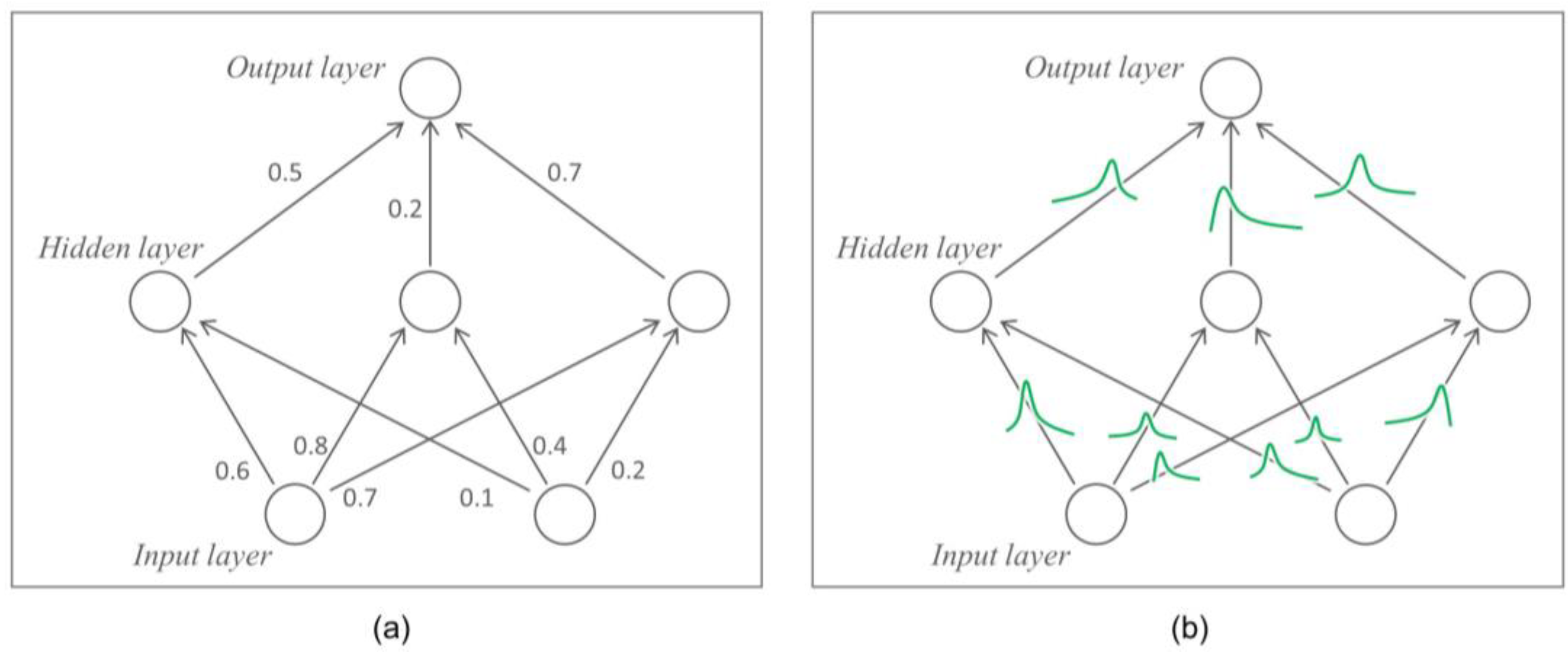
Figure 1a shows the simple DNN architecture. DNN predicts a data label with the fixed weight
that is learned using a training dataset.
Here, let us assume that neural network used in an autonomous driving system determines “stop” and “go” based on the front image. In this example, the neural network learns as it receives a large number of images as input data . A modern DNN can learn without overfitting the training dataset while eliminating the vanishing gradient for nonlinear separable spaces using BP, ReLU, and dropout. Let us assume that random images are inputted into the learned DNN. Then, , which is a predictive value of the DNN, is either “go” and “stop”. That is, a fixed weight-based DNN has a tendency to be overconfident in the training dataset.
DNN is used in areas that are closely associated with human life such as autonomous driving and healthcare. However, given the potential for accidents due to overconfident DNNs of the training dataset, an alternative is now needed. BNN, which handles a weight
that connects layers as random variables is one of the alternatives of DNN [
45,
46,
47,
48].
Figure 1b shows the BNN architecture. The most crucial difference between DNN and BNN is the viewpoint of weight
. In contrast with DNN that uses a fixed weight, weight
is assumed as a random variable of
in BNN. Thus, BNN estimates a probability distribution
with Bayes’ theorem. However, because the operation of posterior in Bayes’ theorem is intractable, it is difficult for BNN training to converge. To overcome this, various tractable mechanisms were proposed such as Wan et al. (2013)’s DropConnect [
49] including dropout and Kingma et al. (2015)’s reparameterization trick [
50,
51].
BNN predicts a sample label using various weights
that are extracted from
. That is, BNN cannot measure the uncertainty of the prediction. Thus, BNN helps the analyzer to make the right decision by increasing the uncertainty of prediction if an unseen case emerges in a training dataset. Wen et al. (2018) introduced Flipout, pointing out that the existing BNN is difficult to learn as the variance of the gradient is high because all training samples in the mini-batch share the same perturbation [
52]. Let us assume that there is a weight
that follows
where
and
refer to mean weights and stochastic perturbation, respectively. Let us also assume
. Then, Flipout ensures the decreasing variance of gradient estimates. Under the training sample
, one entry
of stochastic gradient
can be expressed in Equation (1):
where
is a random variable that depends on
and
.
Let us assume that
is a gradient averaged over a size of mini-batch
. Then, by using the law of total variance,
can be decomposed into the variance of the exact mini-batch gradients and the estimation variance for a fixed mini-batch (see Equations (2)–(4)).
In Equation (2),
refers to the variance of the gradients on individual samples. In Equation (3),
refers to the covariance of the estimation of stochastic perturbation
. As Flipout aims to remove perturbation that is shared in the mini-batch samples,
is removed.
in Equation (4) refers to the term of covariance in . Thus, Flipout trains each layer independently by decreasing and .
4. Proposed Method
This study focuses on estimating the uncertainty of factors that are used to evaluate technologies. Let us assume that factors
and value
of
technologies follow data distribution
. Let us also assume that the value of technology that is classified with the binary class is
. When the value of technology is high,
is 1. Then, BNN
evaluates the technology through input
and weights
. Here, if probability
is larger than the threshold
, the sample is classified to
and vice versa (
is 0 or 1). The estimator of uncertainty about input
whose true label is
is presented in Equation (5):
where
refers to the predicted label of the sample whose true label is
.
This study assumes four research hypotheses. First, the distribution of evaluation factors will differ depending on the technological value. This hypothesis implies that factors can classify technologies clearly according to their value. Second, the BNN’s layer will follow a specific distribution. We assume a layer’s distribution when learning a BNN through the proposed method. If the learning of BNN is adequate, the layer would be approximated to the assumed distribution. Third, the performance of BNN will be better than other classifiers. This study estimates the uncertainty of evaluation factors through BNN. Thus, a BNN whose performance is better than other predictive models would increase the reliability of estimation. Finally, the uncertainty of technology whose value is evaluated as excellent will be higher for more recent technology is more recent. The adequate evaluation of technology requires timeliness and objectivity more than immediacy. Furthermore, evaluation factors may be affected by the time flow. Thus, we assume that the uncertainty of technology, which has been evaluated as excellent in recent years, would be high.
Hypothesis 1. The quantitative factors of patents have different distributions depending on the technology’s value.
The proposed methodology aims to predict technology’s value using quantitative factors and estimate the uncertainty of the factors. Generally, factors such as “number of forward citations” and “number of family patents” are used to evaluate technologies.
The average of the
-th factor
for the
-th sample whose label is
is presented in Equation (6):
where
refers to the sample size where
is
.
Equation (7) presents the variance of each factor depending on the technology’s value.
Thus, Hypothesis 1 means that the difference between
and
according to
is statistically significant. Thus, the null hypotheses we assume are as follows:
where the equality and inequality signs of the alternative hypotheses are defined as the opposite to those of the null hypotheses.
Equation (8) is rejected if the factor of a patent whose technology’s value is high is larger than that whose technology’s value is low. Equation (9) means there is no difference in the deviation of the distribution depending on the technology’s value by comparing the deviation of the factor.
Hypothesis 2. The layers of the Bayesian neural network follow a specific probability distribution.
The proposed methodology predicts the technology’s value using a BNN. This study assumes that the weight
of the layer in the BNN follows the standard normal distribution. Let us assume that random variable
conditioned on
:
. Then, Hypothesis 2 assumes Equation (10).
where the alternative hypothesis for Hypothesis 2 is that weight
does not fall within the standard normal distribution.
When Equation (10) cannot be rejected, the mean and variance of will be approximated to 0 and 1, respectively. Their skewness and kurtosis are also close to 0.
Hypothesis 3. The Bayesian neural network has higher prediction performance than other models.
Hypothesis 3 assumes that the performance of BNN would be higher than that of other classifiers. BNN can measure a loss of samples
times through the layer distribution. Thus, the loss of BNN is calculated by Equation (11).
where
and
refer to the distribution of
and the
-th measured loss of the sample.
Here, let
be the loss of a predictive model other than BNN. Then, the null hypothesis for Hypothesis 3 is Equation (12).
where the alternative hypothesis for Hypothesis 3 is that
is less than
.
By rejecting Equation (12), we can ensure that the reliability of the estimation of uncertainty and the BNN performance is better than other predictive models.
Hypothesis 4. The uncertainty in highly valued technology increases over time.
Technology value is determined by marketability, originality, and scope of rights. However, these factors may be evaluated differently depending on the time when technology development is completed. For example, the number of forward citations tends to be smaller for patents that are more recently registered. Furthermore, technologies that were developed in the past may attract attention a decade later. Thus, we assume that the uncertainty of technology evaluation would fluctuate depending on the timeliness and objectivity of the technology. Then, the null hypothesis for Hypothesis 4 is given by Equation (13).
According to Hypothesis 4, the uncertainty of technology value that is evaluated more recently is higher than those that are not recent. In general, existing IP-R&D did not consider when the technology value is evaluated. However, the technology evaluation of recently registered patents would fluctuate more. Thus, it is essential to establish an IP-R&D strategy according to the time of technology evaluation.
Our study aims to estimate the uncertainty when evaluating a technology using factors that contain technology features. BNN has an advantage in that it can predict technology value several times for the same sample as it learns a distribution of weights. Using this, we estimate the uncertainty of the factors. Let us assume
the gradient averaged over a mini-batch
as the random variable obtained in the learning process. When
is
,
is given by Equation (14).
where
denotes the gradient under the perturbation
for Sample
[
52].
Flipout helps the layer distribution of each factor to be independent of each other. To achieve this, the proposed method aims to reduce the expected variance estimation of individual data points and covariance of layer distribution. Equation (15) presents the variance of that is calculated through Flipout in the proposed method.
5. Experimental Results
The purpose of the experiment is to study the applicability of the proposed method. We collected a patent dataset consisting of 3781 healthcare cases. In this section, we explain (i) the preparation process for the experiment, (ii) the statistical test on the research hypotheses, and (iii) the feature ablation trial.
5.1. Experimental Setup
We collected 3781 patents for healthcare, which were filed in the United States Patent and Trademark Office (USPTO). Data-based healthcare has been applied in a wide range of areas in recent years [
53]. In particular, incorrect analysis in healthcare can lead highly risky such as the prediction of oxygen saturation [
54] or clinical interpretation of somatic mutations in cancer [
55]. Thus, the evaluation of healthcare technologies must be objective and rigorous.
Table 2 presents the evaluation factors extracted from the collected patents. The factors from
num_app to
num_ipc are factors that explain the features of the patents as well as the predictors of the predictive model. The
value in the table indicates the target variable of the patent value. The
value refers to the technology value provided in the patent database, which is classified into High (or 1) and Low (or 0). Thus, we designed a binary-class classification model that predicts a target variable with patent predictors.
Table 3 presents the data splitting results to train the BNN. The test dataset comprises 30% of 3781 cases. The rest of the data were split into training and validation datasets in the proportion 8:2. The BNN trained the training dataset and employed the validation dataset to prevent overfitting. The performance of the model whose learning was completed was measured using the test dataset.
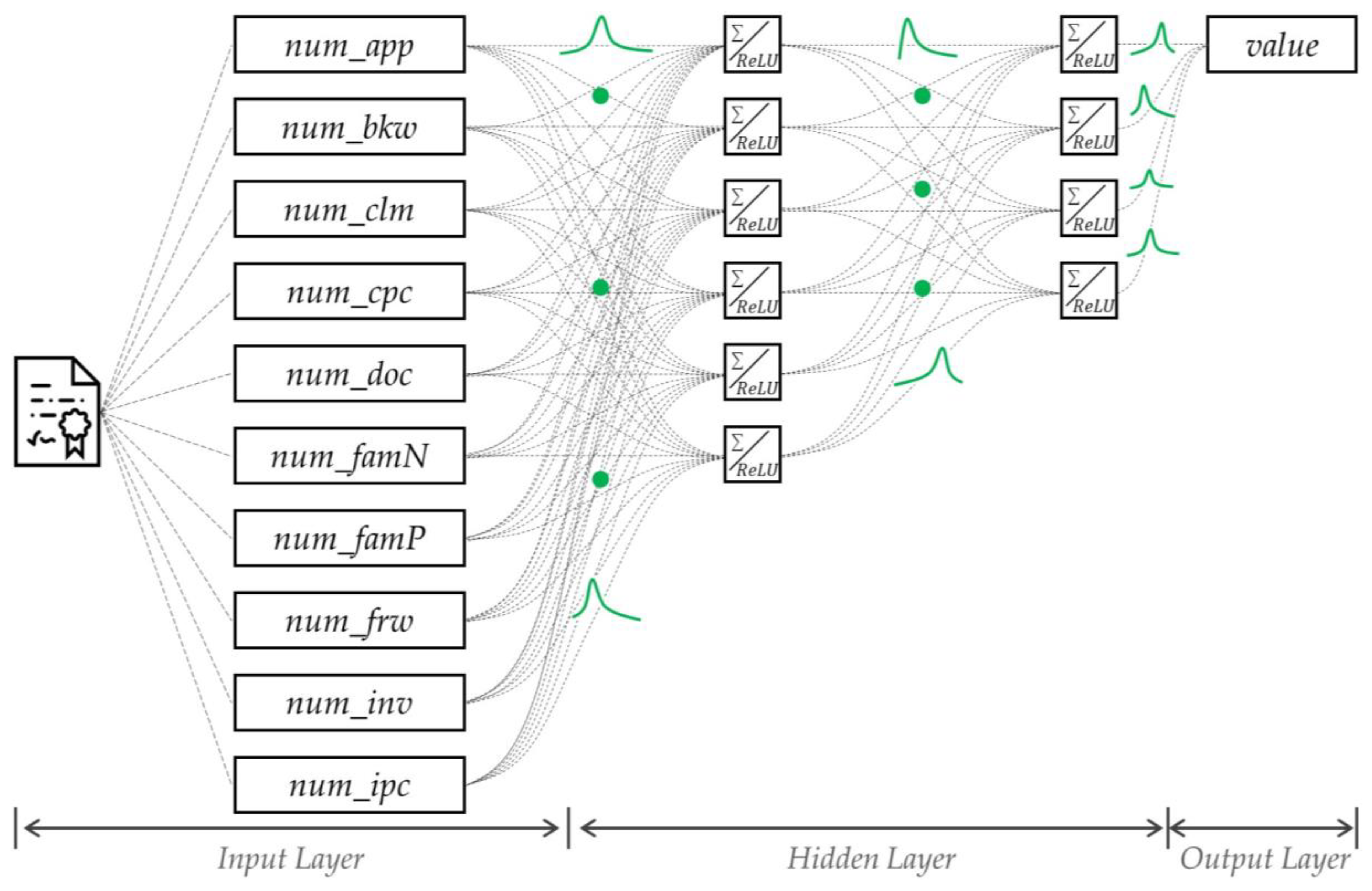
The BNN architecture used in the experiment is as follows: The number of neurons in the input layer is 10, and the number of neurons in the two hidden layers are 6 and 4. The ReLU was used as the activation function in the layer. The model was learned to minimize a negative log loss. In the learning, 256 mini-batch sizes and 50 epochs were used. The Kullback–Leibler divergence was employed to approximate the layer distribution.
Figure A1 in
Appendix A shows the detailed architecture of BNN.
5.2. Statistical Test for Research Hypothesis
In this study, four research hypotheses were proposed in order to prove the validity of our method. We prove the proposed hypotheses using statistical tests. The statistical tests were conducted sequentially from Hypotheses 1 to 4. All statistical hypotheses were tested at the 0.05 significance level.
5.2.1. Statistical Test for Hypothesis 1
Hypothesis 1 assumes that the evaluation factors of patents would have a statistically significant impact on the determination of technology value.
Table 4 presents the statistical test results according to the factors. For example, if we calculate the average and standard deviation of the number of backward citations (
num_bkw) for patents whose value is high, they are 79.099 and 259.065. In contrast, the average and standard deviation of
num_bkw of patents whose
value is low are 34.435 (
) and 86.937 (
).
In the table, ‘Levene’ refers to the p-value of Levene’s test to test the equal variance of the factors according to the value. ‘T-test’ and ‘Wilcoxon’ refer to the p-values of the parametric and nonparametric methods to test whether the averages of the factors are equal according to the value. At the significance level of 0.05, the num_bkw of patents whose value is high is more than that of patents whose value is low. Thus, num_bkw can be viewed as a statistically adequate factor that can differentiate the technology’s value of the patents. The statistical test result of Hypothesis 1 showed that factors other than num_app, num_inv, and num_ipc had a significant impact on determining the technology’s value of the patents.
5.2.2. Statistical Test for Hypothesis 2
Hypothesis 2 assumes that after training the BNN, the layer distribution is approximated to a normal distribution. Through this hypothesis, we can prove the adequacy of the training.
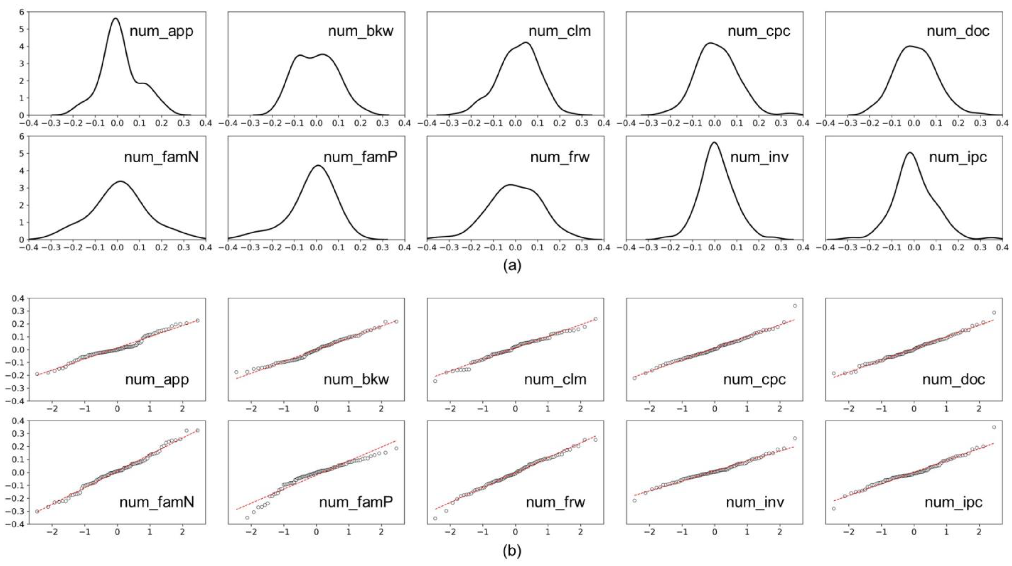
Figure 2a shows the joint probability density distribution of the layer of each factor.
Figure 2b shows the quantile–quantile plot (Q–Q plot) of the distribution of each layer. The results showed that most distributions of the factors were approximated to a normal distribution.
Table 5 presents the statistical test results of Hypothesis 2. We measured the average, standard deviation, skewness, and kurtosis of each layer’s distribution. The average and standard deviation of the standard normal distribution are 0 and 1, and their skewness and kurtosis are both 0. The comparison results of the basic statistics showed that the skewness and kurtosis of
num_famP were significantly different in the standard normal distribution.
The Shapiro–Wilk test of the technology evaluation factors revealed that
num_app,
num_famP, and
num_ipc rejected the null hypothesis at the significance level of 0.05 [
56]. Thus, the distribution of the layer other than that of the above three factors can be viewed as following a normal distribution.
5.2.3. Statistical Test for Hypothesis 3
Hypothesis 3 assumes that the performance of the BNN would be higher than that of other predictive models. This ensures that the BNN not only estimates the uncertainty of the evaluation but also enables accurate prediction. The experiments were conducted to compare the performance of BNN and other predictive models. The comparison models were logistic regression (LR), decision tree (DT), and k-nearest neighbors (KNN). The Gini index was used to split a decision tree, and the number of neighbors used in KNN was five.
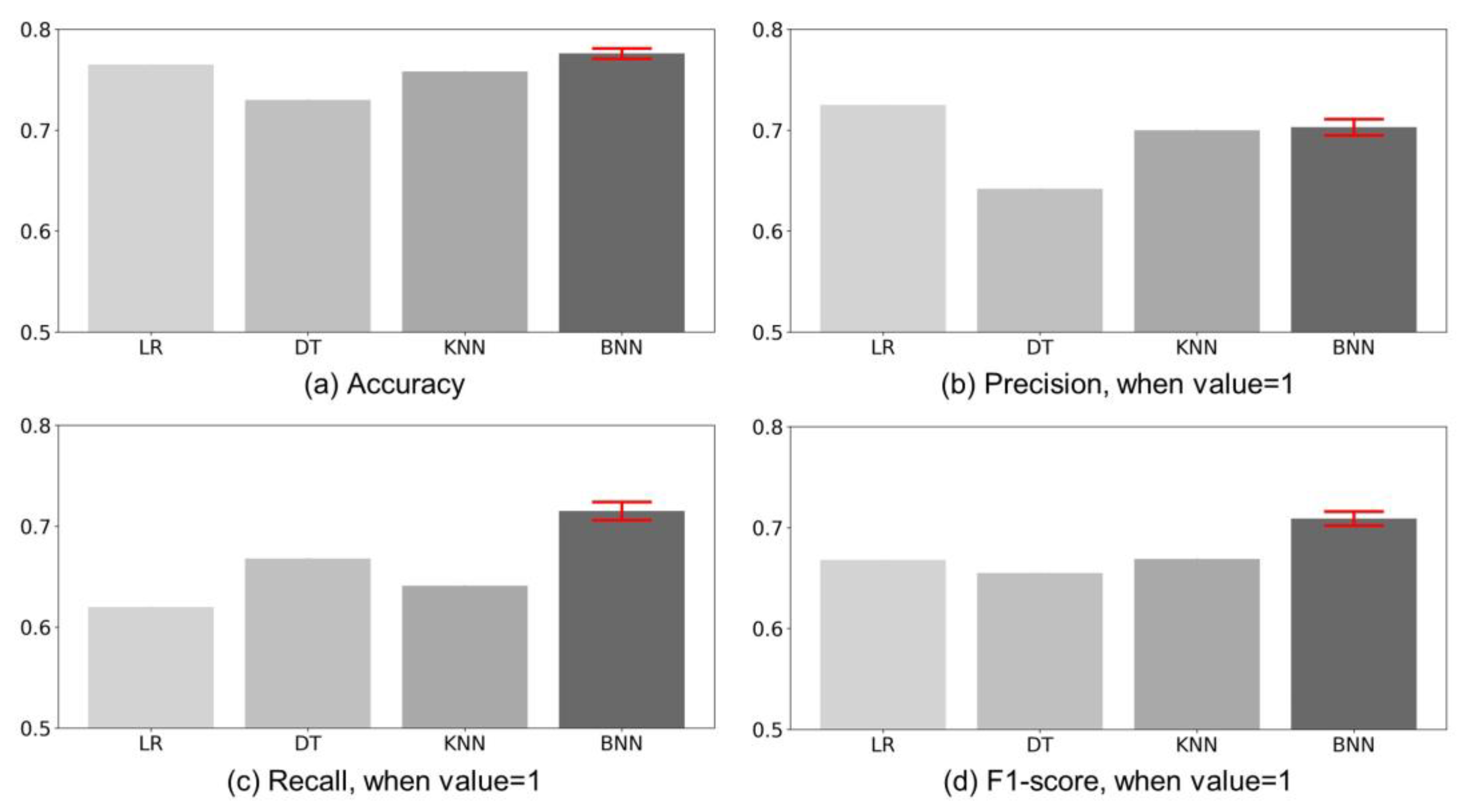
Figure 3 shows the comparison charts of (a) Accuracy, (b) Precision, (c) Recall, and (d) F1-score, which are indicators that measure the performance of the models. BNN calculated the prediction interval using the average and deviation, which was measured ten times (
) iteratively for the test dataset. In Accuracy, BNNs perform similarly to LRs. However, other performance of LR shows that the model’s predictions are biased. The F1-score is an indicator showing the performance corrected for the bias of prediction. BNN’s F1-score is higher than other classifiers. Specifically, BNN ([0.702, 0.716]), KNN (0.669), LR (0.668), and DT (0.655) are high in that order. The performance of BNN is up to 109.31% higher than other classifiers. Moreover, the range of variation is very small. In other words, BNN is (
i) faster than prediction through expert evaluation, (
ii) less costly, and (
iii) stable prediction is possible. Thus, BNN can be seen as an adequate predictive model to estimate the uncertainty of the evaluation.
5.2.4. Statistical Test for Hypothesis 4
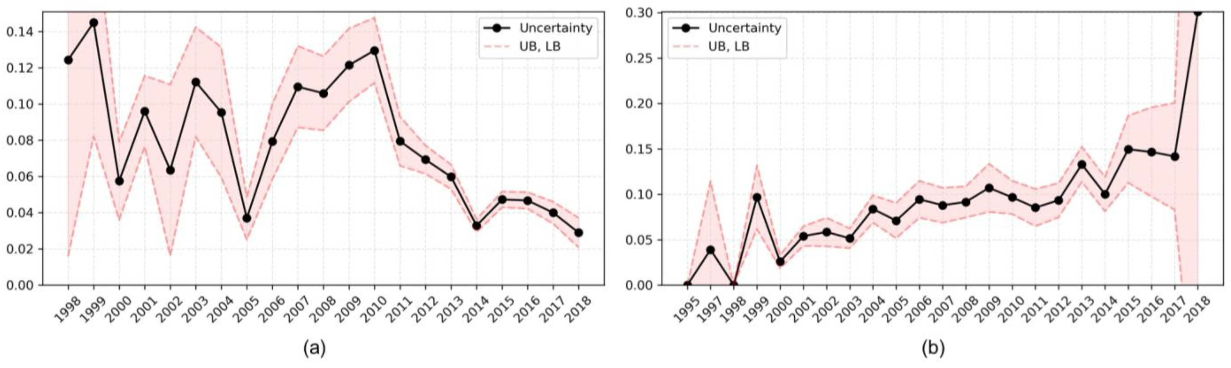
Figure 4a shows the visualized results of the uncertainty according to the patent application year of patents whose value is low. BNN measured the uncertainty of patents whose technology value was low in the past very highly and vice versa.
Figure 4b shows the uncertainty based on the application year of patents whose value is high. BNN measured the uncertainty of patents whose technology value was high in recent years very highly. Thus, researchers should be careful not to be overconfident regarding patents whose value is high among the recently invented technologies.
Table 6 presents the statistical test results of the uncertainty’s trend according to the patent application year. When the value was low, the results tended to decrease statistically significantly in the Spearman and Kendall rank correlation test. In contrast, when the value was high, the results tended to increase in the statistical test. Thus, the uncertainty of patents whose value was high gradually increased over time at the significance level of 0.05.
The experimental results using the patent data of healthcare exhibited that most factors had a significant impact on the evaluation of technology. Furthermore, the BNN’s weight, which learned patent data, followed a normal distribution, and its performance was better than that of other classifiers. The experiments also showed that the uncertainty of the technology’s value of recently registered patents was higher than that of the patents registered in the past.
5.3. Factor Ablation Trial
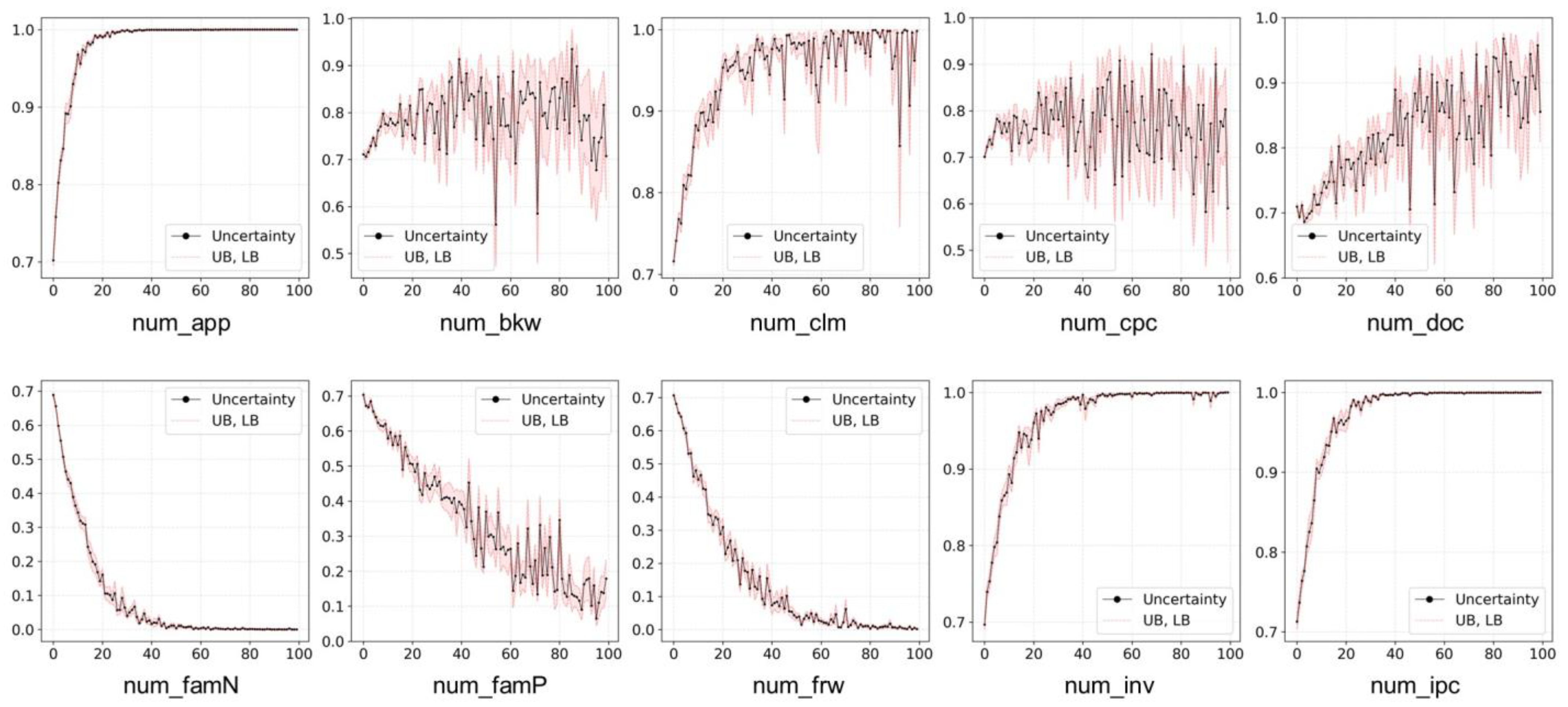
The purpose of the ablation study in deep learning is to observe the change in performance by removing a particular factor or layer in the network. This study aimed to measure the change in uncertainty by entering a random value to the factor in the BNN through the factor ablation trial. First, the operation of BNN for the rest of the factors except for the -th factor is ignored. Then, the change in is observed iteratively while increasing the value of the -th factor from 0 to 100.
Figure 5 shows the results of the factor ablation trial. In the figure, the black line indicates the uncertainty of evaluation according to the factor. The red line denotes the upper bound (UB) and lower bound (LB) of fluctuating uncertainty. Through a factor ablation trial, we measured the degree to which the uncertainty of evaluation changes as the value of the factor increases.
Variables num_app, num_clm, num_doc, num_inv, and num_ipc showed an increasing trend of uncertainty of technology evaluation as the factor increased. In contrast, the uncertainty of evaluation decreased as num_famN, num_famP, and num_frw increased. In addition, num_bkw and num_cpc did not show a clear trend of increase or decrease in the uncertainty. Nevertheless, num_bkw and num_cpc had the lowest uncertainty around 60 and 90, respectively.
The results of the statistical test on the factor ablation trial are summarized in
Table 7. We tested whether the trend of the uncertainty according to the change in the factors was increasing or decreasing using the Spearman and Kendall rank correlation test. At the significance level of 0.05, the results showed that factors
num_frw,
num_famN, and
num_famP contributed to decreasing the uncertainty of evaluation.
The validation of the experiment is as follows:
As a result, BNN had the highest F1-score, followed by KNN, LR, and DT. This means that the performance has improved by up to 109.31% compared to the previous one. Since the range of fluctuation of BNN performance is very small, the proposed method can make stable predictions.
We found a trend in uncertainty over time. This means that when researchers build IP-R&D strategies, they must consider the period when the value of the technology was evaluated.
Through the feature ablation trial, we found that the uncertainty of evaluation decreased as num_famN, num_famP, and num_frw among the factors increased. In addition, we found that num_app, num_clm, num_doc, num_inv, and num_ipc are proportional to the uncertainty of evaluation.
Through experiments, we were able to discover empirical evidence for the proposed research hypothesis. The strengths and weaknesses discovered along the way are discussed in the remaining sections.
6. Discussion
The importance of technology has been emphasized by various firms, universities, and research institutions in modern society. Specifically, firms search for their strengths or competitors’ weaknesses through technologies. Patents are one of the important cornerstones to conducting IP-R&D because they exhibit the history of technological advances as well as predict the future vision.
Patents have been widely used to evaluate technological values in existing studies. They employed factors such as patent citations, claims, and family patents to train predictive models. However, as the importance of timeliness and objectivity is emphasized more than the immediacy of technology evaluation, it is necessary to have a study on methods to measure the uncertainty of the prediction.
The proposed method set four research hypotheses to estimate the uncertainty of technology evaluation factors. The first hypothesis was that factors would affect the technology value. The second hypothesis was that BNN learning would be adequate. The third hypothesis was that the BNN performance would be higher than that of other classifiers. The final hypothesis was that the more recent the evaluated value was, the higher the uncertainty was.
Empirical evidence obtained from statistical tests on the hypotheses is as follows:
Technology value is determined by originality, marketability, and the scope of rights.
The causal relationship of technology value with the number of applicants who own patent rights, the number of inventors, and the number of IPC codes should be carefully interpreted.
Nonetheless, the evaluation of technology, which is higher in the number of countries for family patents, the number of forward citations, and the number of family patents, can be trusted more than that of other cases.
This study proposed a method to estimate the uncertainty of technology evaluation through Bayesian-based predictive models. Our experiments on the proposed method were conducted by collecting healthcare patents, which were likely to have a high risk of technology evaluation. We statistically tested four hypotheses using 3781 cases of data. The test results of the first hypothesis confirmed that there was a statistically significant difference in technology evaluation factors according to the patent value. More specifically, all factors except for the number of applicants who own patent rights, the number of inventors, and the number of IPC codes were fit to evaluate technologies.
Through the experiment results, we verified that the BNN layer, which learned healthcare-related patents, was approximated to the statistical distribution. The performance measurement results of technology evaluation exhibited that BNN had the highest F1-score ([0.702, 0.716]), followed by KNN (0.669), LR (0.668), and DT (0.655). We also verified that the uncertainty of the recently evaluated technology value was high. We discovered in the feature ablation trial that the larger the values of the number of countries for family patents (Spearman’s statistics, −0.973), the number of forward citations (Spearman’s statistics, −0.972), and the number of family patents (Spearman’s statistics, −0.949), the lower the uncertainty of technology evaluation. Thus, the results implied that these three factors were the important ones to determine the technology value.
This study estimated the uncertainty of factors used to evaluate the technology. IP-R&D is conducted in various ways, not only through technology evaluation but also technology transfer, vacant technology, and emerging technology. Thus, it is necessary to measure and compare the uncertainty of the tasks used in various IP-R&D strategies in future studies. Through this, we expect our study results to contribute to a wide range of IP-R&D activities.
7. Conclusions
Innovative technologies can be used by firms to develop new business models. Consequently, firms are interested in various IP-R&D activities such as the prediction of technology transfer, vacant technology, and emerging technology. Conventionally, IP-R&D was conducted through discussions between experts. However, this approach has a limitation that the result may differ depending on the experts’ opinions. Much attention has been paid to the data-based approach by researchers because it can overcome this limitation.
Some researchers have focused on the fact that patents can be linked to citations and proposed a method using a social network. Other researchers have used machine learning or deep learning to predict the future technology value. However, the aforementioned approaches cannot estimate the uncertainty of modeling. Therefore, this study proposed a method that (i) ensures IP-R&D objectivity, (ii) predicts the future, and (iii) estimates the uncertainty.
This study has certain limitations:
Patents are documents that describe the technology. However, we did not use patent texts.
We predicted patent value through BNN. We also compared the performance with that of other classifiers. However, although our model was the best, it was not good enough to be applied to the real world.
More recently, various layers have been proposed as deep learning advances. However, this was not considered.
Therefore, the future research directions we propose are as follows:
In recent years, the study field of natural language processing has rapidly grown. Thus, it is necessary to consider the patent text when estimating technology value in future studies.
Prediction performance needs to be further improved. Reliable prediction performance helps discover new technology opportunities beyond technology evaluation in various fields.
We need to compare the estimation of uncertainty according to various layers in future studies. This is because the attention-based layer suitable for the patent document helps the model understand the technical terms of the patent [
57].
We did not improve the prediction performance using various layers (e.g., convolutional layer) that is used in deep learning or patent texts. Nonetheless, we proposed various hypotheses to estimate the uncertainty of technology evaluation and verified the empirical evidence. Thus, we expect our contribution to be helpful for IP-R&D for the next industrial revolution.


