A Fractional-Order Improved Quantum Logistic Map: Chaos, 0-1 Testing, Complexity, and Control

Abstract

Based on a quantum logistic map and a Caputo-like delta difference operator, a fractional-order improved quantum logistic map, which has hidden attractors, was constructed. Its dynamical behaviors are investigated by employing phase portraits, bifurcation diagrams, Lyapunov spectra, dynamical mapping, and 0-1 testing. It is shown that the proposed fractional-order map is influenced by both the parameters and the fractional order. Then, the complexity of the map is explored through spectral entropy and approximate entropy. The results show that the fractional-order improved quantum logistic map has stronger robustness within chaos and higher complexity, so it is more suitable for engineering applications. In addition, the fractional-order chaotic map can be controlled for different periodic orbits by the improved nonlinear mapping on the wavelet function.

1. Introduction

Since May presented the logistic map in 1976, and as a well-known chaotic map, the logistic map and its generalizations have gained more and more attention in academic circles, especially regarding chaos and fractals [1,2,3]. A quantum logistic map that is associated with the logistic map is proposed in [4]. As a three-dimensional map, it was found that the quantum logistic map owns richer dynamical behaviors, and thus it has greater potential application in the field of information security. However, when compared to the logistic map, there has been relatively less research into quantum logistic maps. The generalization of quantum logistic maps has never been analyzed, so we have investigated it.

In recent years, the theory of the fractional differential equation has become a new research focus. The author of [5] introduced fractional LTI systems, and [6] investigated the existence of a mild-solution Hilfer fractional-neutral-integro-differential inclusion with almost sectorial operators. The authors of [7] studied the existence, uniqueness, Hyer–Ulam stability, and controllability of a fractional dynamic system using time scales, and [8] analyzed the existence, uniqueness, and stability of a nonlinear fractional differential equation with impulsive conditions on time scales. The dynamics of a fractional–order model with different strains of COVID-19 were explored in [9]. The new field of fractional differential equations emerged via the discretized definitions of continuous fractional derivatives and integrals [10,11,12,13]. With the rapid development of the fractional difference equations theory, the definition of fractional-order difference was introduced into discrete chaotic maps based on the Caputo operator, and the fractional standard map and the fractional logistic map were proposed [14,15]. Since then, researchers have diverted their interest to fractional-order chaotic maps. The authors of [16,17,18] presented fractional-order logistic maps and fractional-order delayed logistic maps and analyzed their nonlinear behaviors by using phase portraits, bifurcation diagrams, and Lyapunov exponents. The authors of [19] designed an efficient image encryption scheme based on the fractional-order logistic map, while those of [20] put forward a fractional-order Hénon-Lozi map and then studied its dynamical properties. A two-dimensional fractional-order map was designed and applied to image encryption [21]. A fractional-order higher-dimensional multicavity chaotic map was studied in [22]. Fractional-order chaotic maps are sensitive to their fractional order apart from their initial values and parameters, thereby having richer nonlinear behaviors than the integer-order versions. Hence, a generalized quantum logistic map with fractional order is presented in the paper.

On the other hand, the chaotic system with hidden attractors is a new research hotspot. Some chaotic systems with hidden attractors were presented in the literature [23,24,25]. If a chaotic system possesses no equilibrium or stable equilibrium, i.e., its attraction basin does not connect with the neighborhood of the equilibrium, the chaotic system is regarded as a chaotic system with hidden attractors [26,27]. The hidden attractor is considerably important in science and engineering due to the occurrence of unexpected behaviors. The term “hidden attractors” originates from the research of continuous chaotic systems [28,29]. When compared with continuous chaotic systems, the investigation of chaotic maps with hidden attractors has seen a lack of investigation, especially for fractional-order maps with hidden attractors; they are rarely introduced in the literature. However, the fractional-order map owns more complex dynamical behaviors than the integer counterpart. In order to enrich the theory of hidden attractors, we propose a fractional-order improved quantum logistic map without equilibrium, i.e., a fractional-order map with hidden attractors. For future applications, its behaviors are explored by nonlinear tools, such as bifurcation diagrams and Lyapunov exponents. Moreover, the chaos control of this fractional-order map is also studied.

The remainder of this paper is outlined as follows. Section 2 gives a fractional-order improved quantum logistic map. Section 3 shows the dynamical analysis of the fractional-order map by exploiting bifurcation analysis, Lyapunov exponent spectrums, dynamical maps, and 0-1 tests. Section 4 focuses on the complexity of this map. Section 5 investigates the chaos control of the system. We draw conclusions in Section 6.

2. A Fractional-Order Improved Quantum Logistic Map

A quantum logistic map is a logistic map with quantum corrections [4]. In order to investigate the effects of these quantum corrections, researchers set $\widehat{a}=\langle \widehat{a}\rangle +\delta \widehat{a}$, where $\delta \widehat{a}$ is a quantum fluctuation about $\langle \widehat{a}\rangle$, and $\langle \widehat{a}\rangle$ is the mean value of $\widehat{a}$. The quantum logistic map is described as

$$\{\begin{array}{l}{x}_n=r(x_{n-1}-{\left|x_{n-1}\right|}^2)-r{y}_{n-1},\hfill \\ y_n=-y_{n-1}{e}^{-2\beta }+e^{-\beta }r[(2-x_{n-1}-x_{n-1}^{*})y_{n-1}-x_{n-1}{z}_{n-1}^{*}-x_{n-1}^{*}{z}_{n-1}],\hfill \\ z_n=-z_{n-1}{e}^{-2\beta }+e^{-\beta }r[2(1-x_{n-1}^{*})z_{n-1}-2x_{n-1}{y}_{n-1}-x_{n-1}],\hfill \end{array}$$

(1)

where $x=\langle \widehat{a}\rangle$, $y=\langle \delta {\widehat{a}}^{+}\delta \widehat{a}\rangle$, $z=\langle \delta \widehat{a}\delta \widehat{a}\rangle$, and x*, z* are the complex conjugate of x, z, respectively. Besides, β and r denote the dissipation and control parameters, respectively. However, if we let the initial values x₀, y₀, and z₀ be real numbers, the successive values x_n, y_n, and z_n remain real. Therefore, Equation (1) is expressed as

$$\{\begin{array}{l}{x}_n=r(x_{n-1}-{\left|x_{n-1}\right|}^2)-r{y}_{n-1},\hfill \\ y_n=-y_{n-1}{e}^{-2\beta }+e^{-\beta }r[(2-2x_{n-1})y_{n-1}-2x_{n-1}{z}_{n-1}],\hfill \\ z_n=-z_{n-1}{e}^{-2\beta }+e^{-\beta }r[2(1-x_{n-1})z_{n-1}-2x_{n-1}{y}_{n-1}-x_{n-1}],\hfill \end{array}$$

(2)

For the quantum logistic map, the map has one fixed-point: (0, 0, 0). In order to design a chaotic system with hidden attractors, Equation (2) is rewritten as

$$\{\begin{array}{l}{x}_n=f(x_{n-1})-r_1{y}_{n-1},\hfill \\ y_n=-y_{n-1}{e}^{-2\beta }+e^{-\beta }r[(2-2x_{n-1})y_{n-1}-2x_{n-1}{z}_{n-1}],\hfill \\ z_n=-z_{n-1}{e}^{-2\beta }+e^{-\beta }r[2(1-x_{n-1})z_{n-1}-2x_{n-1}{y}_{n-1}-x_{n-1}],\hfill \end{array}$$

(3)

where r₁ is a parameter, and the function f(x_n−1) is defined as

$$f(x_{n-1})=\{\begin{array}{c}0.8+r{x}_{n-1}(0.2-x_{n-1})\\ if0<x_{n-1}<0.2,\\ r(x_{n-1}-0.8)(1-x_{n-1})\\ if0.8<x_{n-1}<1.\end{array}$$

(4)

For solving the fixed-point of system (3), we have x_n = x_n−1, y_n = y_n−1, and z_n = z_n−1, that is

$$\{\begin{array}{l}{x}_n=f(x_n)-r_1{y}_n,\hfill \\ y_n=-y_n{e}^{-2\beta }+e^{-\beta }r[(2-2x_n)y_n-2x_n{z}_n],\hfill \\ z_n=-z_n{e}^{-2\beta }+e^{-\beta }r[2(1-x_n)z_n-2x_n{y}_n-x_n],\hfill \end{array}$$

(5)

where the function f(x) is described as

$$f(x_n)=\{\begin{array}{c}0.8+r{x}_n(0.2-x_n)if0<x_n<0.2,\\ r(x_n-0.8)(1-x_n)if0.8<x_n<1.\end{array}$$

(6)

The solution of Equation (5) has two cases. When $0<0.8+r{x}_n(0.2-x_n)-r_1{y}_n<0.2$ or $0.8<r(x_n-0.8)(1-x_n)-r_1{y}_n<1$, the first equation can be solved, i.e., the fractional-order map has a fixed-point. If not, there is no solution to the first equation. In other words, the improved map is a system without equilibrium. The second case will be considered below.

Regarding the second and third equations as fractional order, we can obtain

$$\{\begin{array}{cc}\hfill x_n& =f(x_{n-1})-r_1{y}_{n-1},\hfill \\ \hfill { }^C{\Delta }_a^{\nu }y(t)& =-y(t+\nu -1)e^{-2\beta }+e^{-\beta }r[(2-2x(t+\nu -1))y(t+\nu -1)\hfill \\ \hfill & -2x(t+\nu -1)z(t+\nu -1)]-y(t+\nu -1),\hfill \\ \hfill { }^C{\Delta }_a^{\nu }z(t)& =-z(t+\nu -1)e^{-2\beta }+e^{-\beta }r[2(1-x(t+\nu -1))z(t+\nu -1)\hfill \\ \hfill & -2x(t+\nu -1)y(t+\nu -1)-x(t+\nu -1)]-z(t+\nu -1),\hfill \end{array}$$

(7)

where ${ }^C{\Delta }_a^{\nu }$ is the ν-th Caputo-like delta difference operator, ν is the fractional order, and a is the starting point. Set N_a is the isolated time scale, N_a = {a, a + 1, a + 2,...} (a $\in$ R fixed). For ν > 0, ν $\notin$ N, and u(t) define on N_a, the Caputo-like delta difference [30] is defined by

$${}^C{\Delta }_a^{-\nu }u(t)={\Delta }_a^{-(m-\nu )}{\Delta }^{m}u(t), t\in {\mathrm{N}}_{a+m-\mathsf{\nu }},m=\lceil \nu \rceil +1,$$

(8)

where ν is the difference order and ${\Delta }_a^{-\left(m-\nu \right)}$ is the fractional sum of m-ν order. Let u: N_a → R and ν > 0, the fractional sum of ν order [10] is defined by

$${\Delta }_a^{-\nu }u(t)=\frac{1}{\mathsf{\Gamma }(\nu )}{\displaystyle \sum _{s=a}^{t=\nu }{(t-\sigma (s))}^{(\nu -1)}}u(s), t\in {\mathrm{N}}_{a+\mathsf{\nu }},$$

(9)

where σ(s) = s + 1, $\mathsf{\Gamma }\left(\nu \right)$ is the Gamma function, and t(ν) is the falling function defined by the Gamma function as

$$t^{(\nu )}=\frac{\mathsf{\Gamma }(t+1)}{\mathsf{\Gamma }(t+1-\nu )}.$$

(10)

Therefore, the Caputo-like delta difference can be expressed as

$${}^C{\Delta }_a^{-\nu }u(t)=\frac{1}{\mathsf{\Gamma }(m-\nu )}{\displaystyle \sum _{s=a}^{t-(m-\nu )}{(t-\sigma (s))}^{(m-\nu -1)}}{\Delta }^{m}u(s), t\in {\mathrm{N}}_{a+m-\nu }{,}_{ }=\lceil \nu \rceil +1.$$

(11)

According to the theorem in [31], for the difference equation:

$$C{\Delta }_a^{\nu }u\left(t\right)=f\left(t+\nu -1,u\left(t+\nu -1\right)\right),{\Delta }^{k}u(a)=u_k, m =\lceil \nu \rceil +1,k=0,\dots ,m-1.$$

(12)

The equivalent discrete integral equation is described as

$$u(n)=u_0(t)+\frac{1}{\mathsf{\Gamma }(\nu )}{\displaystyle \sum _{s=a+m-\nu }^{t-\nu }{(t-\sigma (s))}^{(\nu -1)}}\times f(s+\nu -1,u(s+\nu -1)), t \in {\mathrm{N}}_{a+m},$$

(13)

where the initial iteration is

$$u_0(t)={\displaystyle \sum _{k=0}^{m-1}\frac{{(t-a)}^{(k)}}{k!}}{\Delta }^{k}u(a).$$

(14)

By setting m = 1, a = 0, and substituting σ(s) = s + 1 into Equation (13), the following can be obtained as

$$u(n)=u_0(t)+\frac{1}{\mathsf{\Gamma }(\nu )}{\displaystyle \sum _{s=1-\nu }^{t-\nu }{(t-s-1)}^{(\nu -1)}}\times f(s+\nu -1,u(s+\nu -1))$$

(15)

By using Equation (10), and setting j = s + ν, Equation (15) is rewritten as

$$u(n)=u_0(t)+\frac{1}{\mathsf{\Gamma }(\nu )}{\displaystyle \sum _{j=1}^n\frac{\mathsf{\Gamma }(n-j+\nu )}{\mathsf{\Gamma }(n-j+1)}}\times f(j-1,u(j-1))$$

(16)

According to Equation (16), the explicit numerical formula of Equation (7) is expressed as

$$\{\begin{array}{l}{x}_n=f(x_{n-1})-r_1{y}_{n-1},\hfill \\ y_n=y_0+\frac{1}{\mathsf{\Gamma }(\nu )}{\displaystyle \sum _{j=1}^n\frac{\mathsf{\Gamma }(n-j-\nu )}{\mathsf{\Gamma }(n-j-1)}\{-y_{j-1}{e}^{-2\beta }+e^{-\beta }r[(2-2x_{j-1})y_{j-1}-2x_{j-1}{z}_{j-1}]-y_{j-1}\},}\hfill \\ z_n=z_0+\frac{1}{\mathsf{\Gamma }(\nu )}{\displaystyle \sum _{j=1}^n\frac{\mathsf{\Gamma }(n-j-\nu )}{\mathsf{\Gamma }(n-j-1)}}\{-z_{j-1}{e}^{-2\beta }+e^{-\beta }r[2(1-x_{j-1})z_{j-1}-2x_{j-1}{y}_{j-1}-x_{j-1}]-z_{j-1}\},\hfill \end{array}$$

(17)

where the function f(x_n−1) is the same as Equation (4).

For System (17), set the parameters as r = 19.8, r₁ = 0.05, β = 4.5, and ν = 0.90, and the initial conditions as (0.05, 0.02, and 0.05); the chaotic attractors are depicted in Figure 1, which are hidden attractors (see Appendix A for the code of the simulation). In this case, we obtain the largest Lyapunov exponent LLE = 0.5426 via the wolf algorithm.

3. Dynamical Analysis

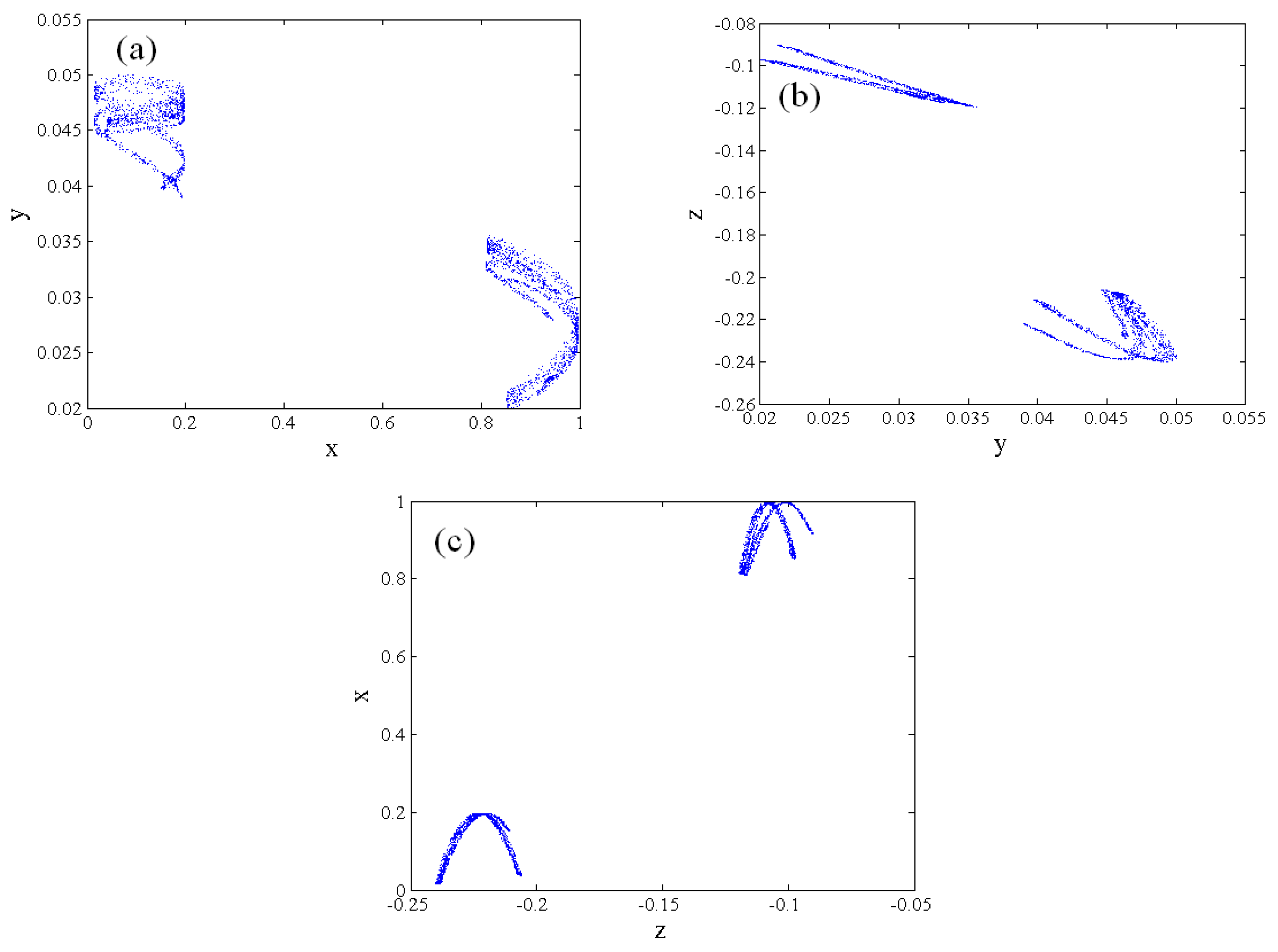
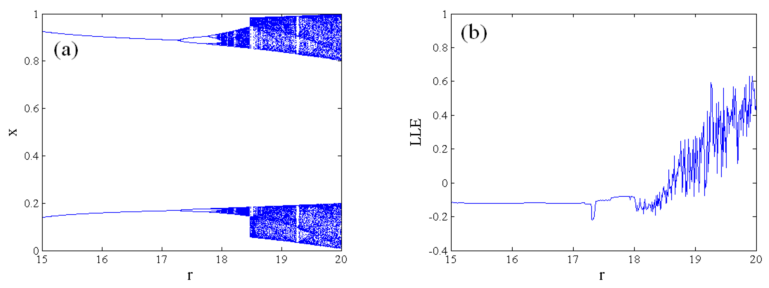
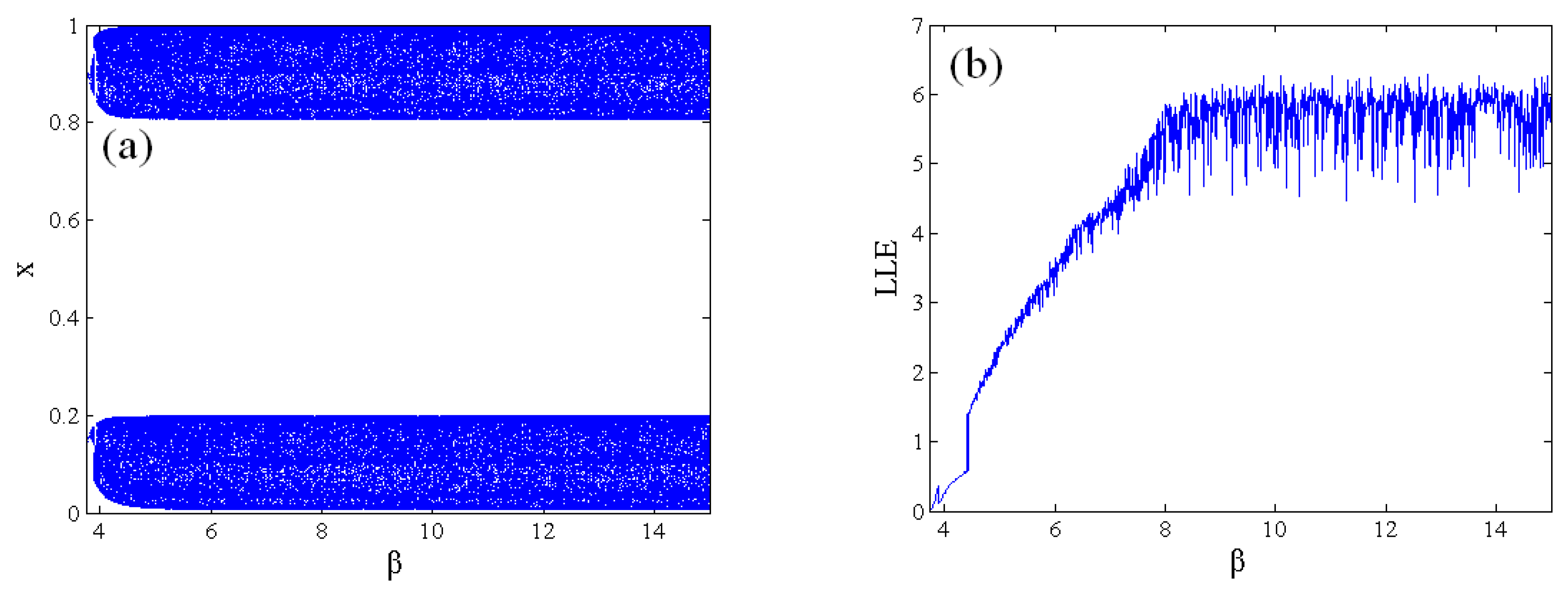
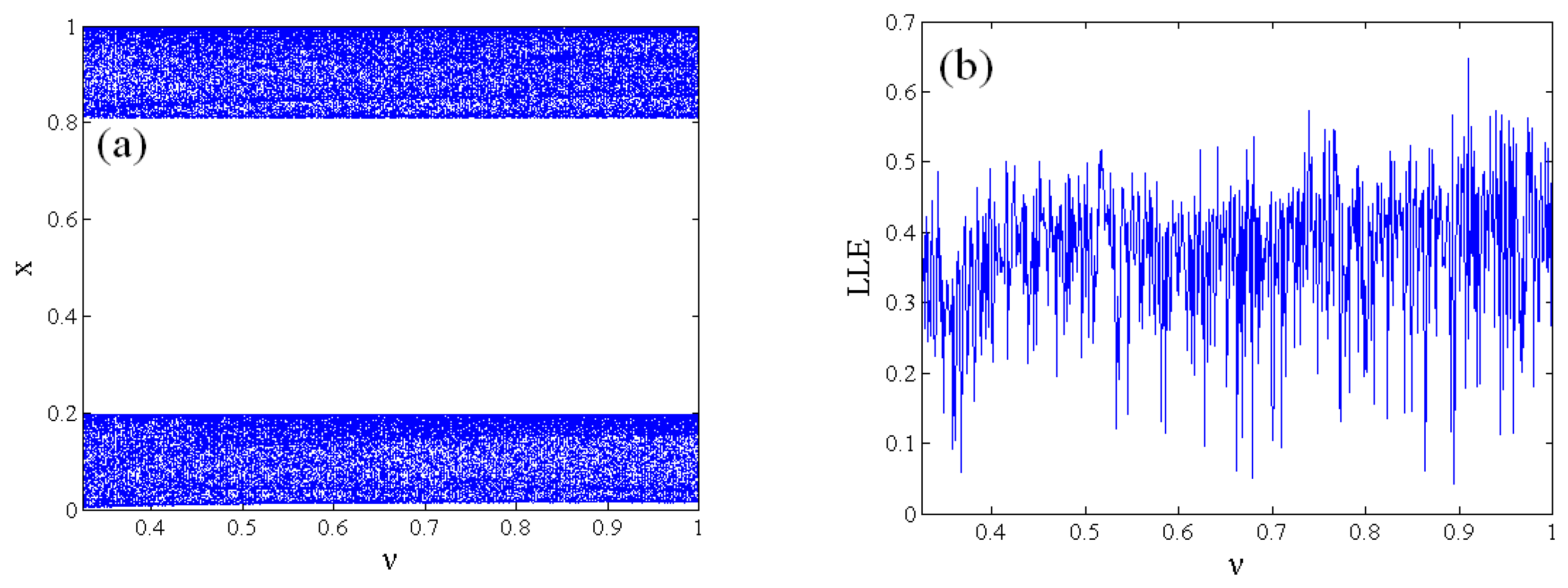
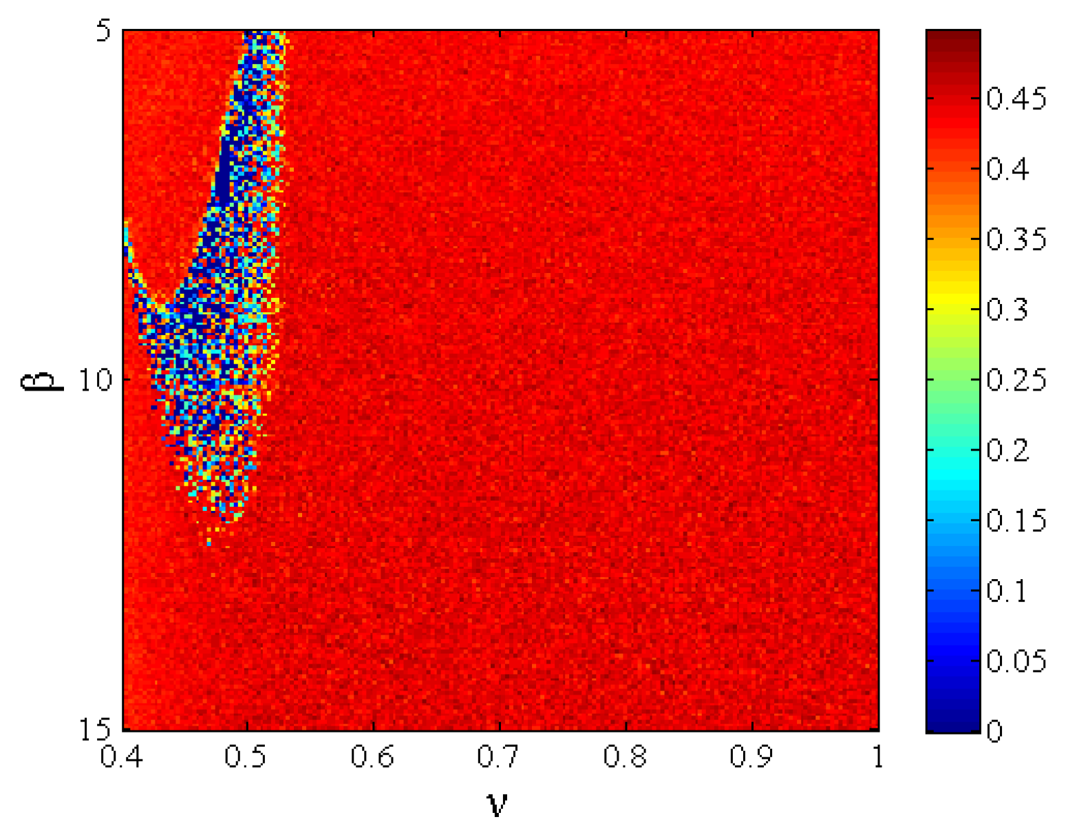
3.1. Bifurcation Analysis, Lyapunov Exponent Spectrum, and Dynamical Map

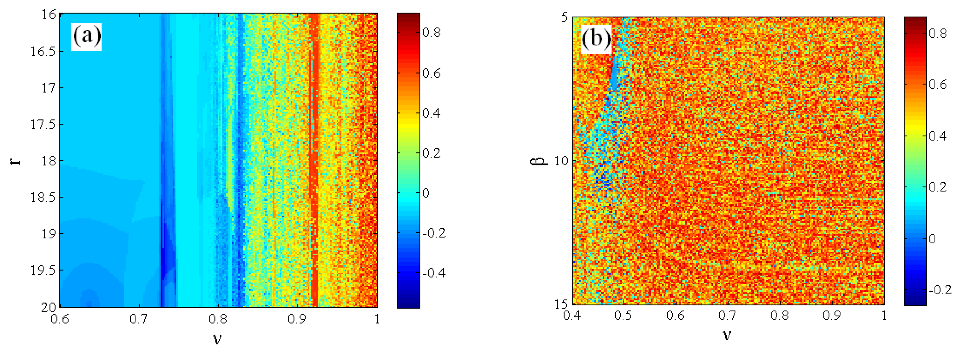
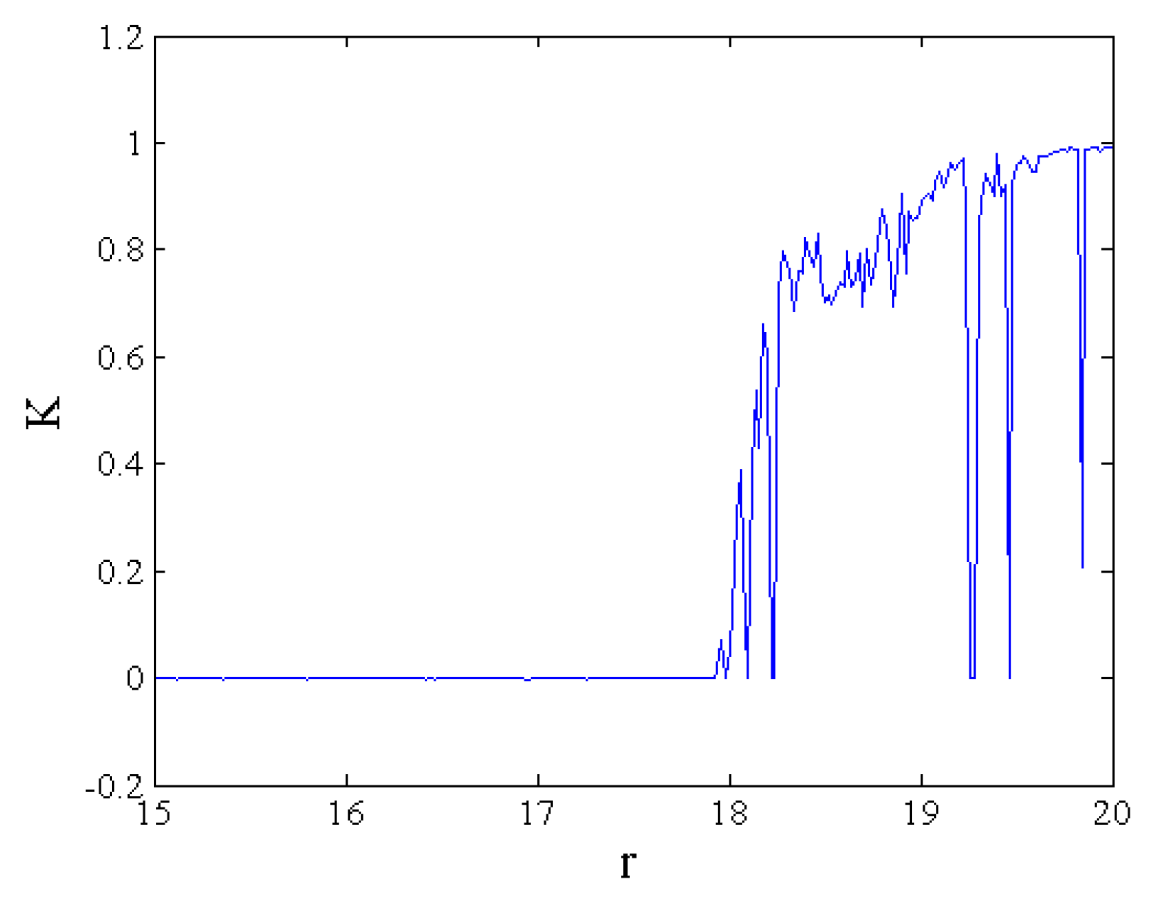
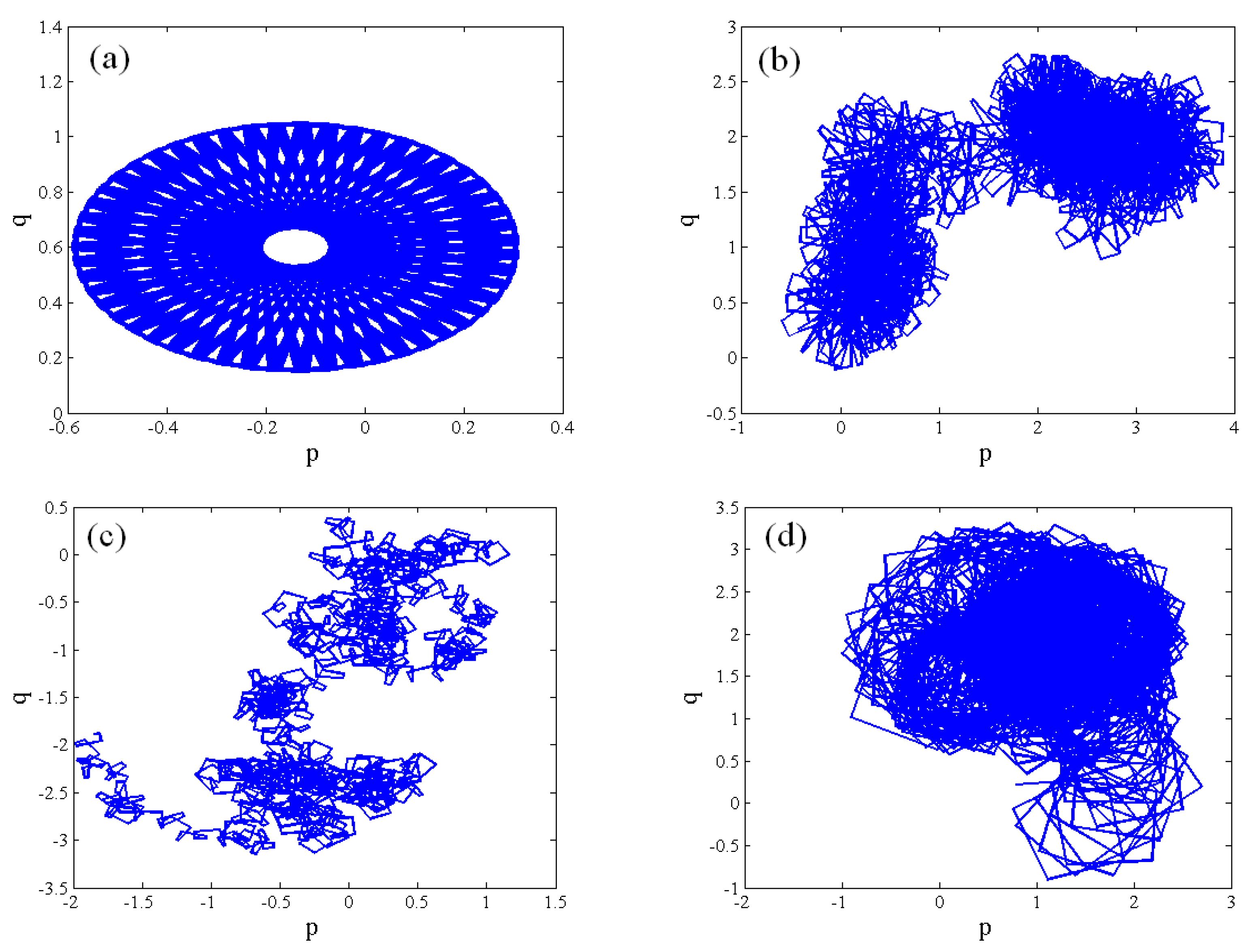
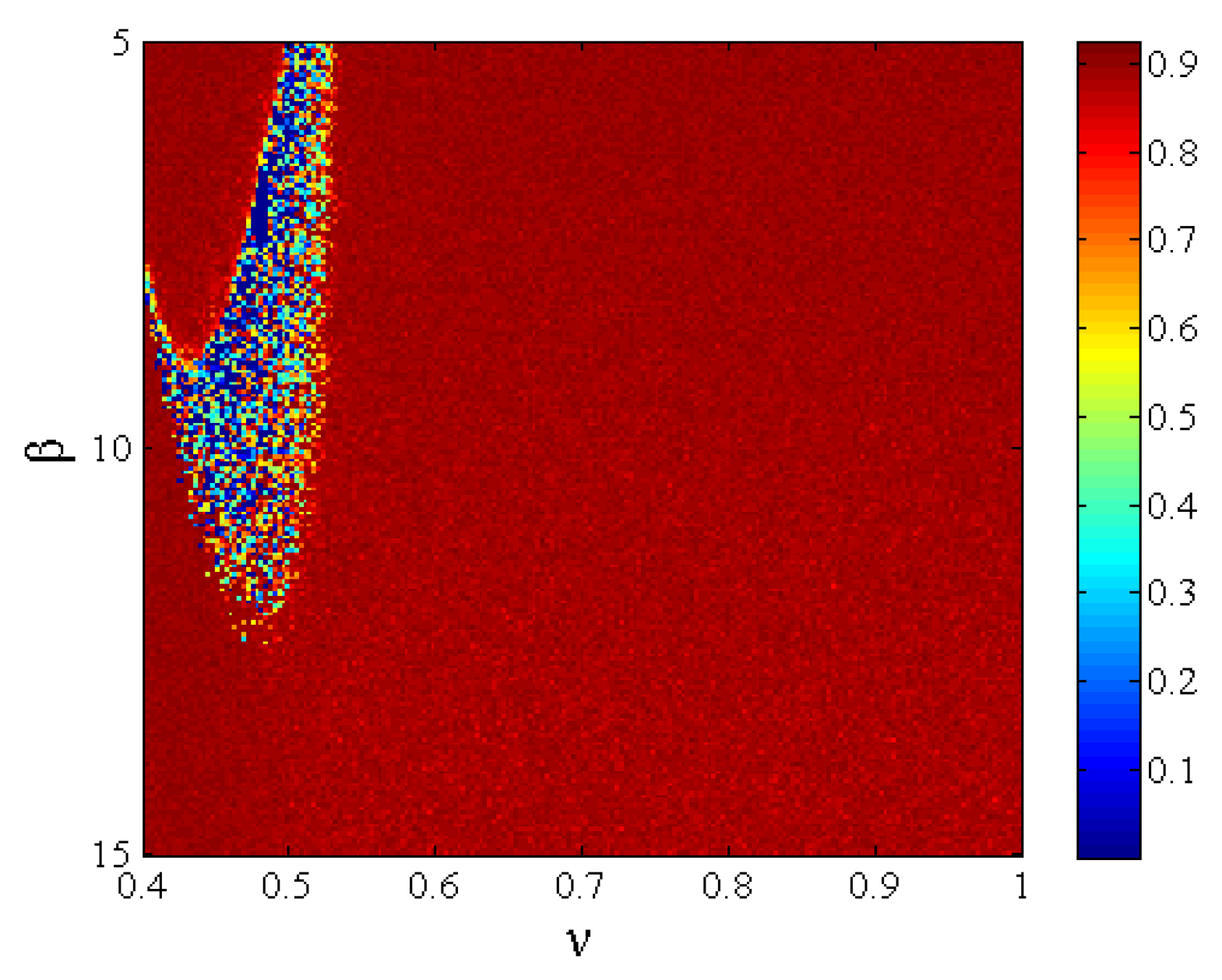
Chaotic maps have sensitivity to the parameters. In order to investigate the sensitivity of the parameters, we fixed the initial conditions as (0.05, 0.02, and 0.05). The bifurcation portrait with respect to the control parameter r and the corresponding largest Lyapunov spectrum is depicted in Figure 2, where the parameter r is in the interval [16,21], and the others are r₁ = 0.05, β = 4.5, and ν = 0.9. It is clear to see that the bifurcation portrait is divided into two parts. With an increase in the parameter r, the system goes through period-2, period-4, a quasi-periodic, and a chaotic state. The system generates periodic windows of different sizes after the system appears in a chaotic state. In the region of $19.2\le r\le 20$, the system keeps a chaotic state.

For the dissipation parameter β, the bifurcation portrait and largest Lyapunov spectrum are plotted in Figure 3 with r = 19.8, r₁ = 0.05, and ν = 0.9. Although the bifurcation portrait shows the phenomenon of bifurcation, the map is mainly in chaotic oscillation. Its chaotic regions are wider than those of the quantum logistic map. When the parameter β is greater than 3.75, the largest Lyapunov exponent is positive, which illustrates that the fractional-order map goes into chaos. When β ∈ (3.75, 8.35], the largest Lyapunov roughly increases with the increasing parameter β. In the range of 8.35 to 15, the largest Lyapunov varies around 5.5. Some of the largest Lyapunov exponents exceed 6, indicating that the map has good nonlinearity and is suitable for information encryption.

Next, we analyze how the fractional order ν influences the map. Figure 4 presents the bifurcation portrait and Lyapunov spectrum versus ν, where the parameters are set as r₁ = 0.05, β = 4.5, r = 1.98, and $0.326\le \nu \le 1$. As can be seen from Figure 4, the largest Lyapunov exponent is always greater than zero, which means that the map remains chaotic. Unlike some other fractional-order chaotic maps [32,33], there are no periodic windows in the chaotic region. Further, the magnitude of the variable x(n) hardly changes with the varying of the fractional order ν. This map demonstrates stronger robustness during chaos than the fractional-order logistic map, the fractional-order Hénon map, and the other fractional-order chaotic maps in [32,33]. When the fractional order is ν < 0.326, the iteration value may not be in the domain of definition. If the iterative value is not in the domain of definition, the iteration will stop. In particular, the phase portrait shows finite points under the condition of ν = 0.2, as shown in Figure 5a, which implies that the iteration stops. On the contrary, Figure 5b exhibits the chaotic attractors with ν = 0.5. However, these chaotic attractors are different from the chaotic attractors shown in Figure 1. The analysis illustrates that the fractional-order map owns richer dynamical behaviors than the integer counterpart.

In order to investigate the influence of the parameters and fractional order on the fractional-order map simultaneously, the dynamical maps are depicted in Figure 6, where the color represents the value of the largest Lyapunov exponent. Figure 6a illustrates the impacts of the control parameters and fractional orders when r₁ = 0.05, β = 10, and (x₀, y₀, z₀) = (0.05, 0.02, 0.05). It is clear to see that the fractional-order map undergoes a change from periodic oscillation to chaos with increasing fractional order. Figure 6b visualizes the influences of the dissipation parameters and fractional orders, where the parameters are set as r = 5 and r₁ = 0.05, and the initial condition is chosen as (x₀, y₀, z₀) = (0.05, 0.02, 0.05). The effects of the dissipation parameters and fractional orders are different from those of the control parameters and fractional orders. The largest Lyapunov exponent in most of the areas is greater than zero, i.e., the system is mainly in a chaotic state.

3.2. 0-1 Test

The 0-1 test is another approach to verify the existence of chaos, which can be utilized directly to a series of data without any phase space reconstruction [34]. Based on the state {x(j)} of System (17), the translation components p_c (n) and q_c (n) are defined as

$$p_c(n)={\displaystyle \sum _{j=1}^{n}x(j)\cos (jc)}, q_c(n)={\displaystyle \sum _{j=1}^{n}x(j)\sin (jc)}$$

(18)

where c is an arbitrary constant in the interval (0, π). By plotting the dynamics of the translation components p_c–q_c, it is easy to determine the state of the system. If p–q trajectories are Brownian-like, the state of the system is chaotic, whereas if the trajectories are bounded, the state is periodic.

Next, the mean square displacement M_c on p_c (n) and q_c (n) is defined as

$$M_c=\underset{N\to \infty }{\lim }\frac{1}{N}{\displaystyle \sum _{j=1}^N\{{[p_c(j+n)-p_c(j)]}^2+{[q_c(j+n)-q_c(j)]}^2}\}, n<<N,$$

(19)

where N is the length of time sequences. In practice, n is chosen as N/10, and the superscript of ∑ is N−n.

Finally, the asymptotic growth rate K_c is calculated by

$$K_c=\underset{n\to +\infty }{\lim }\frac{\log M_c}{\log n}.$$

(20)

We get 100 values for K_c and then let K = median (K_c). When the value of K approaches 0, the system is in a periodic state, and when this value approaches 1, the system is chaotic.

The 0-1 test is performed, and the asymptotic growth rate, K, against r is depicted in Figure 7 under the conditions of r₁ = 0.05, β = 4.5, ν = 0.9, and (x₀, y₀, z₀) = (0.05, 0.02, 0.05). The asymptotic growth rate K is consistent with the bifurcation portrait and the largest Lyapunov spectrum shown in Figure 2. In order to further illustrate the nonlinear behaviors, the p–q trajectories are demonstrated in Figure 8. When r = 17, the bounded trajectory of the p−q plane is shown in Figure 8a, and the asymptotic growth rate is K = 0.0001, implying that the system state is periodic. On the contrary, as r = 19.8, the Brownian-like trajectory is presented in Figure 8b, and the asymptotic growth rate is obtained as K = 0.9958, illustrating that the state is chaotic. Furthermore, the chaotic sequences of r = 19.8 are divided into two sequences according to the value of x_n. The trajectories of 0 < x_n < 0.2 and 0.8 < x_n < 1 are plotted in Figure 8c,d, respectively. The trajectories demonstrate that two sequences keep a chaotic state, so the map can produce multiple chaotic sequences.

4. Complexity and Entropy

4.1. Spectral Entropy

Complexity is an index that is used to measure how well a chaotic system generates random sequences, and larger complexity implies more randomness for the generated sequences. The complexity of the fractional-order map is evaluated by means of spectral entropy (SE). The spectral entropy algorithm [35] is defined as follows; consider a set of time sequences {x_n, n = 0, 1, 2, ..., N − 1} with a length of N, and obtain a new discrete number of length N by subtracting the mean of this dataset, which is expressed as

$$x_n=x_n-\frac{{\displaystyle \sum _{n=0}^{N-1}{x}_n}}{N},$$

(21)

The Fourier transformation is calculated by

$$X_k={\displaystyle \sum _{n=0}^{N-1}{x}_n{e}^{-j2n\pi k/N}},$$

(22)

where k = 0, 1, 2, ..., N − 1 and j is the unit imaginary. The probability of the power spectrum is given as

$$P_k=\frac{{\left|X_k\right|}^2}{{\displaystyle \sum _{k=0}^{N/2-1}{\left|X_k\right|}^2}},$$

(23)

Then, the normalization spectral entropy is defined as

$$SE=\frac{{\displaystyle \sum _{k=0}^{N/2-1}\left|P_k\ln (P_k)\right|}}{\ln (N/2)}$$

(24)

We utilize spectral entropy to measure the complexity of the fractional-order map, and the result of SE complexity is presented in Figure 9. The SE complexity surpasses 0.85 in the highest range, so this fractional-order map can generate better random sequences.

4.2. Approximate Entropy

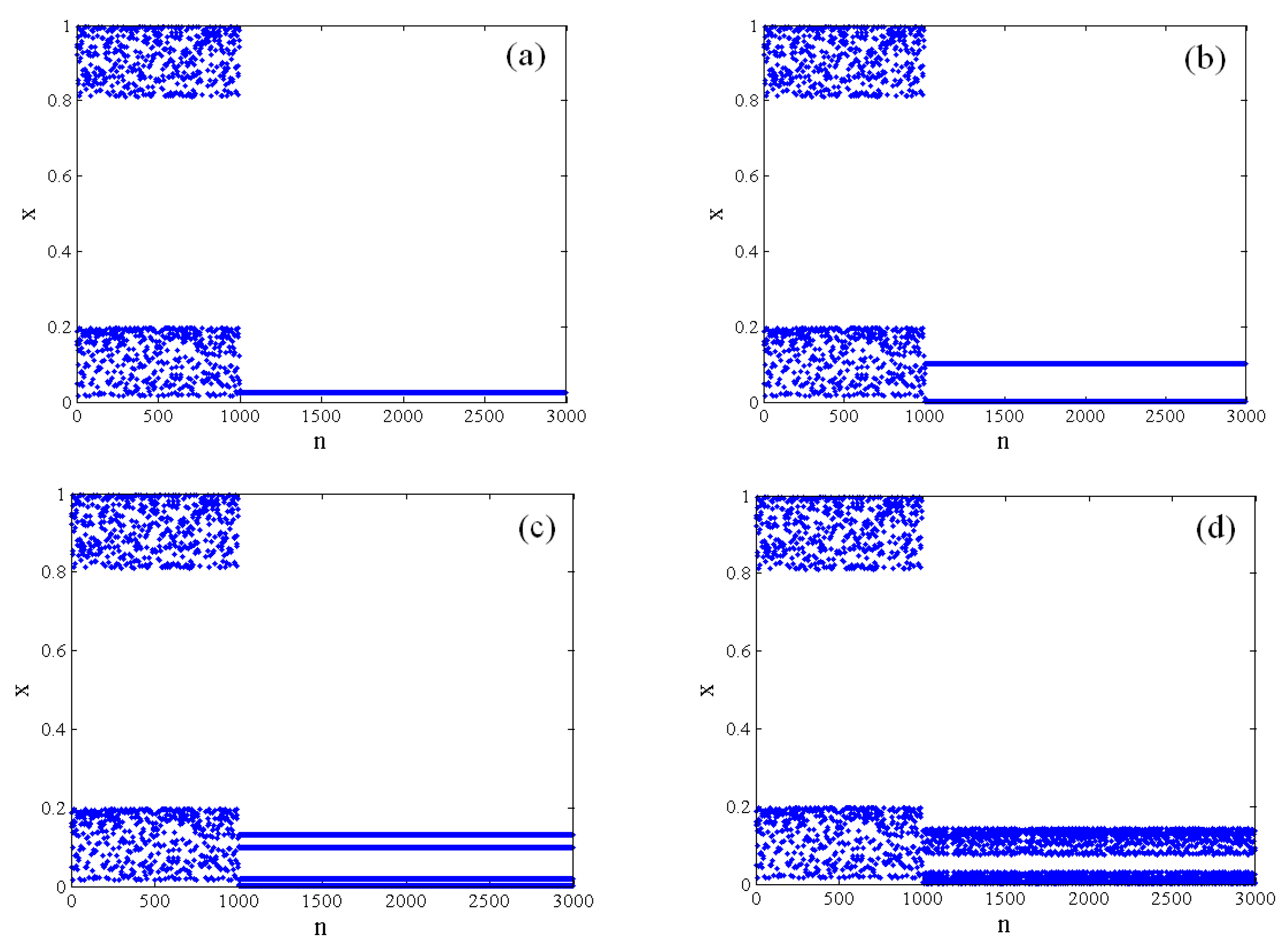
The approximate entropy (ApEn) [36] is the other means to measure the complexity of the fractional-order map, which is described as follows. Consider a set of time sequences x₁, x₂,..., x_n obtained from System (17) and determine n − m +1 vectors as follows:

$$X_i=\left[x_i,x_{i+1}\cdots \cdots x_{i+m-1}\right].$$

(25)

These vectors denote m consecutive x values, which start from the ith data. Giving tolerance, r, and for each $i\in [1,n-m+1]$, we define the following equation:

$$C_i^m(r)=\frac{K}{n-m+1},$$

(26)

in which K is the number of X_i with $d(X_i,X_j)\le r$. In this case, d(X_i, X_j) represents the largest absolute difference between X_i, and X_j. We calculate the approximate entropy by

$$APEn={\varphi }^m(r)-{\varphi }^{m+1}(r),$$

(27)

where ${\varphi }^m(r)$ is described as

$${\varphi }^m(r)=\frac{1}{n-m-1}{\displaystyle \sum _{i=1}^{n-m+1}\log C_i^m(r)},$$

(28)

The result of ApEn complexity is shown in Figure 10, which agrees well with SE complexity. Therefore, this fractional-order map has a more complex structure. It has higher complexity than the fractional-order logistic map and the fractional-order Hénon map.

5. Chaos Control

As the fractional-order chaotic map is raised, the chaos control for the fractional-order map becomes a new topic. The occurrence of chaotic behaviors may cause instability in engineering applications, so chaos control has been widely studied. However, researchers have paid little attention to the topic of controlling fractional-order chaotic maps. In the section, the scheme of chaos control is proposed, which is based on improved nonlinear mapping on wavelet functions [37]. System (17) is controlled by it. This control method of fractional-order systems is of importance not only for control theory, but also for the application of fractional-order chaotic maps. A Marr wavelet function is employed to construct the improved nonlinear mapping. This chaos control algorithm is described as

$$\{\begin{array}{cc}\hfill x_n& =k{e}^{-\frac{x_{n-1}^2}{2}}(1-x_{n-1}^2)[f(x_{n-1})-r_1{y}_{n-1}],\hfill \\ \hfill { }^C{\Delta }_a^{\nu }y(t)& =-y(t+\nu -1)e^{-2\beta }+e^{-\beta }r[(2-2x(t+\nu -1))y(t+\nu -1)\hfill \\ \hfill & -2x(t+\nu -1)z(t+\nu -1)]-y(t+\nu -1),\hfill \\ \hfill { }^C{\Delta }_a^{\nu }z(t)& =-z(t+\nu -1)e^{-2\beta }+e^{-\beta }r[2(1-x(t+\nu -1))z(t+\nu -1)\hfill \\ \hfill & -2x(t+\nu -1)y(t+\nu -1)-x(t+\nu -1)]-z(t+\nu -1),\hfill \end{array}$$

(29)

where k is a control parameter.

If System (17) is controlled when n = 1000, then the control results are presented in Figure 11. The fractional-order chaotic map is controlled to a period-1 orbit with k = 0.2; it is controlled to a period-2 orbit with k = 0.5, and it is controlled to period-4 orbit with k = 0.65, while it is controlled to quasiperiodic orbit with k = 0.7. As can be seen, the fractional-order chaotic map endures period-1, period-2, period-4, and quasiperiodic states with an increase in the control parameter k.

6. Conclusions

We build an improved quantum logistic map without equilibrium by reforming the classic quantum logistic map. The improved quantum logistic map with hidden attractors is generalized to the fractional case by introducing the Caputo-like delta difference operator. Through a phase portrait, the largest Lyapunov exponent, dynamical mapping, and 0-1 testing, the dynamical characteristics were studied. Both the parameters and fractional orders impact the system. With varying control parameters, the system shows periodic windows. However, for the dissipation parameter and the fractional order, there are no periodic windows in the chaotic region. This means that this chaotic map possesses stronger robustness in chaos, so the system could be applied to generate stable chaotic sequences for secure communication. The 0-1 test shows that this fractional-order map can generate several chaotic sequences. Then, the complexity of the fractional-order map was described by spectral entropy and approximate entropy, which shows that this fractional-order map can generate better random sequences. In addition, improved nonlinear mapping on a wavelet function for the fractional-order map was proposed. This map is controlled to different periodic orbits under different control parameters. The fractional-order map gains more degrees of freedom compared to the integer counterpart, so the fractional-order map has greater potential applications in the engineering field. Due to its higher complexity and stronger robustness in chaos, this fractional-order chaotic map can be employed in information encryptions, such as secret communications and image encryptions. In order to apply the fractional-order improved quantum logistic map, we will focus on designing the image encryption scheme based on this map in the future.

References

1. May, R.M. Simple mathematical models with very complicated dynamics. Nature 1976, 261, 459–467. [Google Scholar] [CrossRef] [PubMed]
2. Munir, F.A.; Zia, M.; Mahmood, H. Designing multi-dimensional logistic map with fixed-point finite precision. Nonlinear Dyn. 2019, 97, 2147–2158. [Google Scholar] [CrossRef]
3. Cánovas, J.; Muñoz-Guillermo, M. On the dynamics of the q-deformed logistic map. Phys. Lett. A 2019, 383, 1742–1754. [Google Scholar] [CrossRef]
4. Goggin, M.; Sundaram, B.; Milonni, P. Quantum logistic map. Phys. Rev. A 1990, 41, 5705. [Google Scholar] [CrossRef]
5. Petráš, I. Fractional-order systems. In Fractional-Order Nonlinear Systems: Modeling, Analysis and Simulation, 1st ed.; Springer: Berlin/Heidelberg, Germany, 2011; pp. 43–54. [Google Scholar]
6. Varun Bose, C.B.S.; Udhayakumar, R. Existence of mild solutions for hilfer fractional neutral integro-differential inclusions via almost sectorial operators. Fractal Fract. 2022, 6, 532. [Google Scholar] [CrossRef]
7. Kumar, V.; Malik, M. Existence, stability and controllability results of fractional dynamic system on time scales with application to population dynamics. Int. J. Nonlin. Sci. Num. 2021, 22, 741–766. [Google Scholar] [CrossRef]
8. Kumar, V.; Malik, M. Existence, uniqueness and stability of nonlinear implicit fractional dynamical equation with impulsive condition on time scales. Nonauton. Dyn. Syst. 2019, 6, 65–80. [Google Scholar] [CrossRef]
9. Baba, I.A.; Rihan, F.A. A fractional–order model with different strains of COVID-19. Phys. A 2022, 603, 127813. [Google Scholar] [CrossRef]
10. Atici, F.M.; Eloe, P.W. Initial value problems in discrete fractional calculus. Proc. Am. Math. Soc. 2009, 137, 981–989. [Google Scholar] [CrossRef]
11. Abu-Saris, R.; Al-Mdallal, Q. On the asymptotic stability of linear system of fractional-order difference equations. Fract. Calc. Appl. Anal. 2013, 16, 613–629. [Google Scholar] [CrossRef]
12. Mohan, J.J.; Deekshitulu, G.V.S.R. Fractional order difference equations. Int. J. Differ. Equ. 2012, 2012, 780619. [Google Scholar] [CrossRef] [Green Version]
13. Wyrwas, M.; Mozyrska, D.; Girejko, E. Stability of discrete fractional-order nonlinear systems with the nabla caputo difference. IFAC Proc. 2013, 46, 167–171. [Google Scholar] [CrossRef]
14. Edelman, M. Fractional maps and fractional attractors part I: α-families of maps. Discontin. Nonlinearity Complex. 2013, 1, 305–324. [Google Scholar] [CrossRef]
15. Edelman, M. Fractional maps and fractional attractors part II: Fractional difference α-families of maps. Discont. Nonlinearity Complex. 2015, 4, 391–402. [Google Scholar] [CrossRef] [Green Version]
16. Wu, G.C.; Baleanu, D. Discrete fractional logistic map and its chaos. Nonlinear Dyn. 2014, 75, 283–287. [Google Scholar] [CrossRef]
17. Wu, G.C.; Baleanu, D. Discrete chaos in fractional delayed logistic maps. Nonlinear Dyn. 2015, 80, 1697–1703. [Google Scholar] [CrossRef]
18. Wu, G.C.; Baleanu, D. Jacobian matrix algorithm for Lyapunov exponents of the discrete fractional maps. Commun. Nonlinear Sci. Numer. Simulat. 2015, 22, 95–100. [Google Scholar] [CrossRef]
19. Zhang, Y.Q.; Hao, J.L.; Wang, X.Y. An efficient image encryption scheme based on S-boxes and fractional-order differential logistic map. IEEE Access 2020, 8, 54175–54188. [Google Scholar] [CrossRef]
20. Ouannas, A.; Khennaoui, A.; Wang, X.; Pham, V.T.; Boulaaras, S.; Momani, S. Bifurcation and chaos in the fractional form of Hénon-Lozi type map. Eur. Phys. J. Spec. Top. 2020, 229, 2261–2273. [Google Scholar] [CrossRef]
21. Liu, Z.Y.; Xia, T.; Wang, Y.P. Image encryption technique based on new two-dimensional fractional-order discrete chaotic map and Menezes-Vanstone elliptic curve cryptosystem. Chin. Phys. B 2018, 27, 030502. [Google Scholar] [CrossRef]
22. Wang, L.; Sun, K.; Peng, Y.; He, S. Chaos and complexity in a fractional-order higher-dimensional multicavity chaotic map. Chaos Soliton. Fract. 2019, 131, 109488. [Google Scholar] [CrossRef]
23. Jafari, S.; Pham, V.T.; Golpayegani, S.M.R.H.; Moghtadaei, M.; Kingni, S.T. The relationship between chaotic maps and some chaotic systems with hidden attractors. Int. J. Bifurcat. Chaos 2016, 26, 1650211. [Google Scholar] [CrossRef]
24. Cui, L.; Luo, W.H.; Ou, Q.L. Analysis and implementation of new fractional-order multi-scroll hidden attractors. Chin. Phys. B 2021, 30, 020501. [Google Scholar] [CrossRef]
25. Chowdhury, S.N.; Ghosh, D. Hidden attractors: A new chaotic system without equilibria. Eur. Phys. J. Spec. Top. 2020, 229, 1299–1308. [Google Scholar] [CrossRef]
26. Jafari, S.; Sprott, J.C.; Nazarimehr, F. Recent new examples of hidden attractors. Eur. Phys. J. Spec. Top. 2015, 224, 1469–1475. [Google Scholar] [CrossRef]
27. Leonov, G.A.; Kuznetsov, N.V. Hidden attractors in dynamical systems: From hidden oscillation in Hilbert-Kolmogorov, Aizerman and Kalman problems to hidden chaotic attractor in Chua circuits. Int. J. Bifurcat. Chaos 2013, 23, 1330002. [Google Scholar] [CrossRef] [Green Version]
28. Leonov, G.A.; Kuznetsov, N.V.; Vagaitsev, V.I. Hidden attractor in smooth Chua systems. Phys. D 2012, 241, 1482–1486. [Google Scholar] [CrossRef]
29. Leonov, G.A.; Kuznetsov, N.V.; Vagaitsev, V.I. Localization of hidden Chua’s attractors. Phys. Lett. A 2011, 375, 2230–2233. [Google Scholar] [CrossRef]
30. Abdeljawad, T. On Riemann and Caputo fractional differences. Comput. Math. Appl. 2011, 62, 1602–1611. [Google Scholar] [CrossRef] [Green Version]
31. Chen, F.; Luo, X.; Zhou, Y. Existence results for nonlinear fractional difference equation. Adv. Differ. Equ. 2011, 2011, 713201. [Google Scholar] [CrossRef]
32. Ouannas, A.; Khennaoui, A.A.; Momani, S.; Pham, V.T.; El-Khazali, R. Hidden attractors in a new fractional-order discrete system: Chaos, complexity, entropy, and control. Chin. Phys. B 2020, 29, 050504. [Google Scholar] [CrossRef]
33. Khennaoui, A.A.; Ouannas, A.; Boulaaras, S.; Pham, V.T.; Azar, A.T. A fractional map with hidden attractors: Chaos and control. Eur. Phys. J. Spec. Top. 2020, 229, 1083–1093. [Google Scholar] [CrossRef]
34. Sun, K.H.; Liu, X.; Zhu, C.X. The 0-1 test algorithm for chaos and its applications. Chin. Phys. B 2010, 19, 110510. [Google Scholar] [CrossRef]
35. Staniczenko, P.P.A.; Lee, C.F.; Jones, N.S. Rapidly detecting disorder in rhythmic biological signals: A spectral entropy measure to identify cardiac arrhythmias. Phys. Rev. E 2009, 79, 011915. [Google Scholar] [CrossRef]
36. Pincus, S.M. Approximate entropy as a measure of system complexity. Proc. Natl. Acad. Sci. USA 1991, 88, 2297–2301. [Google Scholar] [CrossRef] [PubMed]
37. Li, X.; Chu, Y.; Liu, X.; Zhang, J. Control discrete (hyper-)chaotic system using improved wavelet functions. J. Huazhong Univ. Sci. Tech. 2009, 37, 72–74. [Google Scholar]
Figure 1. Chaotic attractors of the fractional-order improved quantum logistic map. (a) x-y phase portrait; (b) y-z phase portrait; (c) z-x phase portrait.
Axioms 12 00094 g001
Figure 2. Bifurcation portrait and Lyapunov exponent spectrum with regard to r; (a) bifurcation portrait with regard to r; (b) Lyapunov exponent spectrum with regard to r.
Axioms 12 00094 g002
Figure 3. Bifurcation portrait and Lyapunov exponent spectrum with regard to β. (a) Bifurcation portrait with regard to β; (b) Lyapunov exponent spectrum with regard to β.
Axioms 12 00094 g003
Figure 4. Bifurcation portrait and Lyapunov exponent spectrum with regard to ν. (a) Bifurcation portrait with regard to ν; (b) Lyapunov exponent spectrum with regard to ν.
Axioms 12 00094 g004
Figure 5. Phase portrait. (a) Phase portrait with ν = 0.2; (b) phase portrait with ν = 0.5.
Axioms 12 00094 g005
Figure 6. Dynamical maps. (a) Dynamical map with regard to ν and r; (b) dynamical map with regard to ν and β.
Axioms 12 00094 g006
Figure 7. Asymptotic growth rate K of the fractional-order map with regard to r.
Axioms 12 00094 g007
Figure 8. The pq trajectories of the fractional-order map. (a) pq trajectories of r = 17; (b) the pq trajectories of r = 19.8; (c) pq trajectories of 0 < xn < 0.2; (d) pq trajectories of 0.8 < xn < 1.
Axioms 12 00094 g008
Figure 9. SE of the fractional-order map with regard to ν and β.
Axioms 12 00094 g009
Figure 10. ApEn of the fractional-order map with regard to ν and β.
Axioms 12 00094 g010
Figure 11. Chaotic controls. (a) Chaotic control with k = 0.2; (b) chaotic control with k = 0.5; (c) chaotic control with k = 0.65; (d) chaotic control with k = 0.70.
Axioms 12 00094 g011
Disclaimer/Publisher’s Note: The statements, opinions and data contained in all publications are solely those of the individual author(s) and contributor(s) and not of MDPI and/or the editor(s). MDPI and/or the editor(s) disclaim responsibility for any injury to people or property resulting from any ideas, methods, instructions or products referred to in the content.