Article

Nonlinear Dynamic Behaviors of the (3+1)-Dimensional B-Type Kadomtsev—Petviashvili Equation in Fluid Mechanics

School of Physics and Electronic Information Engineering, Henan Polytechnic University, Jiaozuo 454003, China
*
Author to whom correspondence should be addressed.
Axioms 2023, 12(1), 95; https://doi.org/10.3390/axioms12010095
Submission received: 29 November 2022 / Revised: 29 December 2022 / Accepted: 10 January 2023 / Published: 16 January 2023
(This article belongs to the Special Issue Nonlinear Dynamics and Complexity)

Abstract

:
This paper provides an investigation on nonlinear dynamic behaviors of the (3+1)-dimensional B-type Kadomtsev—Petviashvili equation, which is used to model the propagation of weakly dispersive waves in a fluid. With the help of the Cole—Hopf transform, the Hirota bilinear equation is established, then the symbolic computation with the ansatz function schemes is employed to search for the diverse exact solutions. Some new results such as the multi-wave complexiton, multi-wave, and periodic lump solutions are found. Furthermore, the abundant traveling wave solutions such as the dark wave, bright-dark wave, and singular periodic wave solutions are also constructed by applying the sub-equation method. Finally, the nonlinear dynamic behaviors of the solutions are presented through the 3-D plots, 2-D contours, and 2-D curves and their corresponding physical characteristics are also elaborated. To our knowledge, the obtained solutions in this work are all new, which are not reported elsewhere. The methods applied in this study can be used to investigate the other PDEs arising in physics.

1. Introduction

Nonlinear partial differential equations (NPDEs) are powerful tools to model various complex phenomena in nature [1,2,3,4,5,6]. How to obtain the exact solution of the NPDEs has always been the purpose of researchers. To this day, some effective methods have been proposed to seek for the exact solution of the NPDEs such as the Bäcklund transformation method [7,8,9,10], Cole—Hopf transformation method [11,12,13,14], variational method [15,16], extended rational sine—cosine and sinh—cosh methods [17,18], Sardar subequation method [19,20], the Kudryashov approach [21,22], extended sinh—Gordon equation expansion method [23,24], trial equation method [25,26], sub-equation method [27,28,29], Wang’s direct mapping method [30], and so on [31,32,33,34,35]. In this work, we aim to study the (3+1)-dimensional B-type Kadomtsev—Petviashvili equation that reads as [36]:
ψ t y ψ x x x y 3 ψ x ψ y x + 3 ψ x z = 0 ,
Equation (1) is a subclass of the Kadomtsev—Petviashvili (KP) hierarchy and is used to describe the weakly dispersive waves in a fluid. ψ = ψ x , y , z , t represents the amplitude or elevation of the relevant wave and is a real function of space x, y, z, and time t. Up to now, many effective methods have been proposed to deal with Equation (1) and some results have been obtained. In [37], two methods, namely the simplest equation method and multiple exp-function method, are used to construct the exact solutions of Equation (1). In [38], one- and two-soliton solutions of Equation (1) are obtained by using the Bäcklund transformations. In [39], the extended homoclinic test technique is employed to study Equation (1) and some new rational breather solutions are found. In [40], the direct algebraic method is adopted and the interaction solutions among solitons, rational waves, and periodic waves are obtained. In [41], the soliton molecules, asymmetric solitons, and some novel hybrid solutions are attained by using the velocity resonance mechanism and the long wave limit method. In [42], the exp-function method aided with symbolic computation is utilized to seek for the anti-kink solutions. However, to our knowledge, the multi-wave complexiton, multi-wave, and periodic lump have not been studied. In addition, the sub-equation method has not been employed to study Equation (1) either. Thus, the objective of this work is to search for the abundant solutions of Equation (1) by means of the Hirota bilinear method and sub-equation method. The results obtained in this work are expected to extend the solutions of the (3+1)-dimensional B-type Kadomtsev—Petviashvili equation. The structure of this article is arranged as follows. In Section 2, the Hirota bilinear equation is developed via the Cole—Hopf transform and the symbolic computation with the ansatz function schemes is utilized to find the multi-wave complexiton solutions, multi-wave solutions, and periodic lump solutions, respectively. In Section 3, the sub-equation method is applied to seek for the traveling wave solutions. In Section 4, the physical characteristics and numerical results of the solutions are presented via the 3-D plots, 2-D contours, and 2-D curves. Finally, the conclusion is provided in Section 5.

2. Cole—Hopf Transform and the Exact Solutions

For constructing the exact solutions of Equation (1), we use the Cole—Hopf transform as:
ψ = 2 ln g x .
Applying this transform, we can obtain the bilinear form of Equation (1) as:
D y D t D x 3 D y + 3 D x D z g g = 0 .
Here, the definition of the operators D x m D t n is [43,44,45,46]:
D x m D t n f g = x x m t t n f x , t g x , t | x = x , t = t .
Additionally, there are:
D x f g = f x g f g x ,
D x 2 f g = f x x g 2 f x g x + f g x x ,
D x 2 f f = 2 f x x f f x 2 ,
D t D x f g = f t x g f t g x f x g t + g t x f ,
……

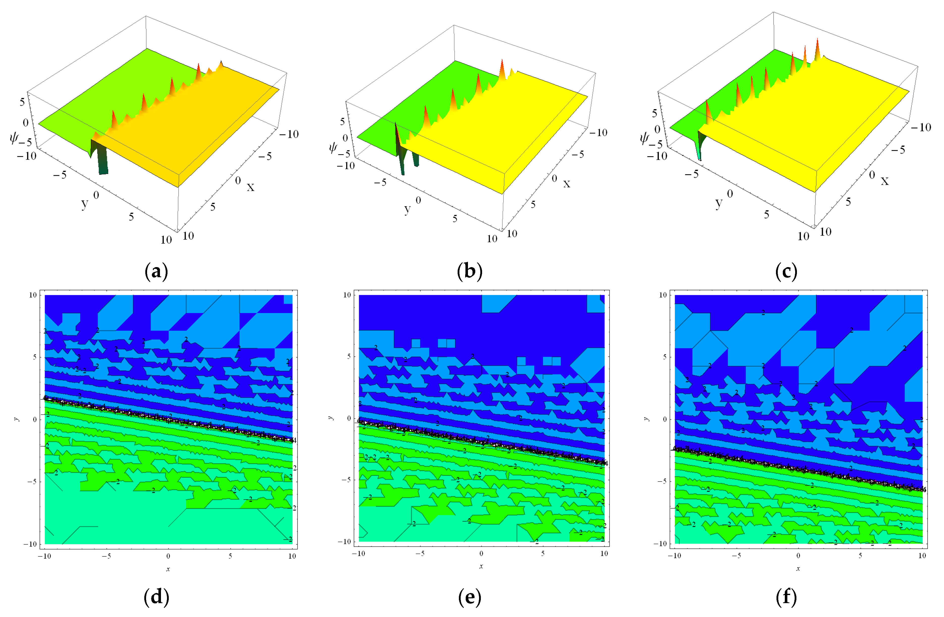
2.1. The Multi-Waves Complexiton Solutions

In order to find the multi-wave complexiton solution, it is assumed that the test function g is:
ϕ = x + ε 1 y + ε 2 z + ε 3 t ,
φ = x + ε 4 y + ε 5 z + ε 6 t ,
γ = x + ε 7 y + ε 8 z + ε 9 t ,
g = Δ 1 e φ + Δ 2 e φ + Δ 3 sin φ + Δ 4 sin h γ ,
where ε i ( i = 1 , 2 , , 9 ) and Δ i ( i = 1 , 2 , 3 , 4 ) are real parameters to be determined later. Substituting Equation (5) into Equation (3) and performing the corresponding adjustments, we have:
  • Case 1:
ε 1 = 3 ε 2 4 ε 9 ,   ε 2 = ε 2 ,   ε 3 = ε 9 ,   ε 4 = 3 ε 2 ε 9 4 ,   ε 5 = ε 2 2 + ε 9 4 ε 9 ,   ε 6 = ε 9 2 ,   ε 7 = 3 ε 2 4 ε 9 ,   ε 8 = ε 2 ,   ε 9 = ε 9 ,   Δ 1 = Δ 1 ,   Δ 2 = Δ 2 ,   Δ 3 = Δ 3 ,   Δ 4 = Δ 4 .
where 4 ε 9 0 . Applying the above results into Equation (5), we can obtain the multi-wave complexiton solution through the transformation provided by Equation (2) as:
ψ ( x , y , z , t ) = 2 [ Δ 1 e x + 3 ε 2 4 ε 9 y + ε 2 z + ε 9 t Δ 2 e ( x + 3 ε 2 4 ε 9 y + ε 2 z + ε 9 t ) + Δ 3 cos ( x + 3 ε 2 ε 9 4 y + ε 2 ( 2 + ε 9 ) 4 ε 9 z + ( ε 9 2 ) t ) + Δ 4 cosh ( x + 3 ε 2 4 ε 9 y + ε 2 z + ε 9 t ) ] [ Δ 1 e x + 3 ε 2 4 ε 9 y + ε 2 z + ε 9 t + Δ 2 e ( x + 3 ε 2 4 ε 9 y + ε 2 z + ε 9 t ) + Δ 3 sin ( x + 3 ε 2 ε 9 4 y + ε 2 ( 2 + ε 9 ) 4 ε 9 z + ( ε 9 2 ) t ) + Δ 4 sinh ( x + 3 ε 2 4 ε 9 y + ε 2 z + ε 9 t ) ]
  • Case 2:
ε 1 = ε 7 ,   ε 2 = ε 2 ,   ε 3 = 4 ε 7 3 ε 2 ε 7 ,   ε 4 = ε 7 ,   ε 5 = 2 ε 7 ε 2 ,   ε 6 = 2 ε 7 3 ε 2 ε 7 ,   ε 7 = ε 7 ,   ε 8 = ε 2 ,   ε 9 = 4 ε 7 3 ε 2 ε 7 ,   Δ 1 = Δ 1 ,   Δ 2 = Δ 2 ,   Δ 3 = Δ 3 ,   Δ 4 = Δ 4 .
Inserting the above results into Equation (5) and using the transformation provided by Equation (2), we can obtain the multi-wave complexiton solution as:
ψ ( x , y , z , t ) = 2 [ Δ 1 e x + ε 7 y + ε 2 z + 4 ε 7 3 ε 2 ε 7 t Δ 2 e x + ε 7 y + ε 2 z + 4 ε 7 3 ε 2 ε 7 t + Δ 3 cos x ε 7 y + 2 ε 7 ε 2 z + 2 ε 7 3 ε 2 ε 7 t + Δ 4 cosh x + ε 7 y + ε 2 z + 4 ε 7 3 ε 2 ε 7 t ] [ Δ 1 e x + ε 7 y + ε 2 z + 4 ε 7 3 ε 2 ε 7 t + Δ 2 e x + ε 7 y + ε 2 z + 4 ε 7 3 ε 2 ε 7 t + Δ 3 sin x ε 7 y + 2 ε 7 ε 2 z + 2 ε 7 3 ε 2 ε 7 t + Δ 4 sinh x + ε 7 y + ε 2 z + 4 ε 7 3 ε 2 ε 7 t ]
  • Case 3:
ε 1 = ε 7 ,   ε 2 = 4 ε 7 3 ε 3 ε 7 3 ,   ε 3 = ε 3 ,   ε 4 = ε 7 ,   ε 5 = ε 3 + 2 ε 7 3 ,   ε 6 = ε 3 2 ,   ε 7 = ε 7 ,   ε 8 = 4 ε 7 3 ε 3 ε 7 3 ,   ε 9 = ε 3 ,   Δ 1 = Δ 1 ,   Δ 2 = Δ 2 ,   Δ 3 = Δ 3 ,   Δ 4 = Δ 4 .
In the same way, we can obtain the multi-wave complexiton solution as:
ψ ( x , y , z , t ) = 2 [ Δ 1 e x + ε 7 y + 4 ε 7 3 ε 3 ε 7 3 z + ε 3 t Δ 2 e x + ε 7 y + 4 ε 7 3 ε 3 ε 7 3 z + ε 3 t + Δ 3 cos x ε 7 y + ε 3 + 2 ε 7 3 z + ε 3 2 t + Δ 4 cosh x + ε 7 y + 4 ε 7 3 ε 3 ε 7 3 z + ε 3 t ] [ Δ 1 e x + e η y + 4 ε r 3 ε 2 η 3 3 + s ^ t + Δ 2 e x + ε 7 y + 4 ε 7 3 ε 3 ε 7 3 z + ε 3 t + Δ 3 sin x ε 7 y + ε 3 + 2 ε 7 3 z + ε 3 2 t + Δ 4 sinh x + ε 7 y + 4 ε 7 3 ε 3 ε 7 3 z + ε 3 t ]
  • Case 4:
ε 1 = ε 7 ,   ε 2 = ε 8 ,   ε 3 = 4 ε 7 3 ε 8 ε 7 ,   ε 4 = ε 7 ,   ε 5 = 2 ε 7 ε 8 ,   ε 6 = 2 ε 7 3 ε 8 ε 7 ,   ε 7 = ε 7 ,   ε 8 = ε 8 ,   ε 9 = 4 ε 7 3 ε 8 ε 7 ,   Δ 1 = Δ 1 ,   Δ 2 = Δ 2 ,   Δ 3 = Δ 3 ,   Δ 4 = Δ 4 .
Accordingly, the multi-wave complexiton solution of Equation (1) is attained as:
ψ ( x , y , z , t ) = 2 [ Δ 1 e x + ε 7 y + ε 8 z + 4 ε 7 3 ε 8 ε 7 t Δ 2 e x + ε 7 y + ε 8 z + 4 ε 7 3 ε 8 ε 7 t + Δ 3 cos x ε 7 y + 2 ε 7 ε 8 z + 2 ε 7 3 ε 8 ε 7 t + Δ 4 cosh x + ε 7 y + ε 8 z + 4 ε 7 3 ε 8 ε 7 t ] [ Δ 1 e x + ε 7 y + ε 8 z + 4 ε 7 3 ε 8 ε 7 t + Δ 2 e x + ε 7 y + ε 8 z + 4 ε 7 3 ε 8 ε 7 t + Δ 3 sin x ε 7 y + 2 ε 7 ε 8 z + 2 ε 7 3 ε 8 ε 7 t + Δ 4 sinh x + ε 7 y + ε 8 z + 4 ε 7 3 ε 8 ε 7 t ]
  • Case 5:
ε 1 = ε 1 ,   ε 2 = ε 8 ,   ε 3 = 4 ε 1 3 ε 8 ε 1 ,   ε 4 = ε 1 ,   ε 5 = 2 ε 1 ε 8 ,   ε 6 = 2 ε 1 3 ε 8 ε 1 ,   ε 7 = ε 1 ,   ε 8 = ε 8 ,   ε 9 = 4 ε 1 3 ε 8 ε 1 ,   Δ 1 = Δ 1 ,   Δ 2 = Δ 2 ,   Δ 3 = Δ 3 ,   Δ 4 = Δ 4 .
Using the above results, we can obtain the multi-wave complexiton solution of Equation (1) via Equation (2) and Equation (5) as:
ψ ( x , y , z , t ) = 2 [ Δ 1 e x + ε 1 y + ε 8 z + 4 ε 1 3 ε 8 ε 1 t Δ 2 e x + ε 1 y + ε 8 z + 4 ε 1 3 ε 8 ε 1 t + Δ 3 cos x ε 1 y + ε 5 z + 2 ε 1 3 ε 8 ε 1 t + Δ 4 cosh x + ε 1 y + ε 8 z + 4 ε 1 3 ε 8 ε 1 t ] [ Δ 1 e x + ε 1 y + ε 8 z + 4 ε 1 3 ε 8 ε 1 + Δ 2 e x + ε 1 y + ε 8 z + 4 ε 1 3 ε 8 ε 1 t + Δ 3 sin x ε 1 y + ε 5 z + 2 ε 1 3 ε 8 ε 1 t + Δ 4 sinh x + ε 1 y + ε 8 z + 4 ε 1 3 ε 8 ε 1 t ]
  • Case 6:
ε 1 = ε 4 ,   ε 2 = ε 4 ε 9 4 3 ,   ε 3 = ε 9 ,   ε 4 = ε 4 ,   ε 5 = 2 ε 4 + ε 4 ε 9 3 ,   ε 6 = ε 9 2 ,   ε 7 = ε 4 ,   ε 8 = ε 4 ε 9 4 3 ,   ε 9 = ε 9 ,   Δ 1 = Δ 1 ,   Δ 2 = Δ 2 ,   Δ 3 = Δ 3 ,   Δ 4 = Δ 4 .
Putting the above results into Equation (5) and using the transformation of Equation (2), we can obtain the multi-wave complexiton solution as:
ψ ( x , y , z , t ) = 2 [ Δ 1 e x ε 4 y + ε 4 ε 9 4 3 z + ε 9 t Δ 2 e x ε 4 y + ε 4 ε 9 4 3 z + ε 9 t + Δ 3 cos x + ε 4 y 2 ε 4 + ε 4 ε 9 3 z + ε 9 2 t + Δ 4 cosh x ε 4 y + ε 4 ε 9 4 3 z + ε 9 t ] [ Δ 1 e x ε 4 y + ε 4 ε 9 4 3 z + ε 9 t + Δ 2 e x ε 4 y + ε 4 ε 9 4 3 z + ε 9 t + Δ 3 sin x + ε 4 y 2 ε 4 + ε 4 ε 9 3 z + ε 9 2 t + Δ 4 sinh x ε 4 y + ε 4 ε 9 4 3 z + ε 9 t ]

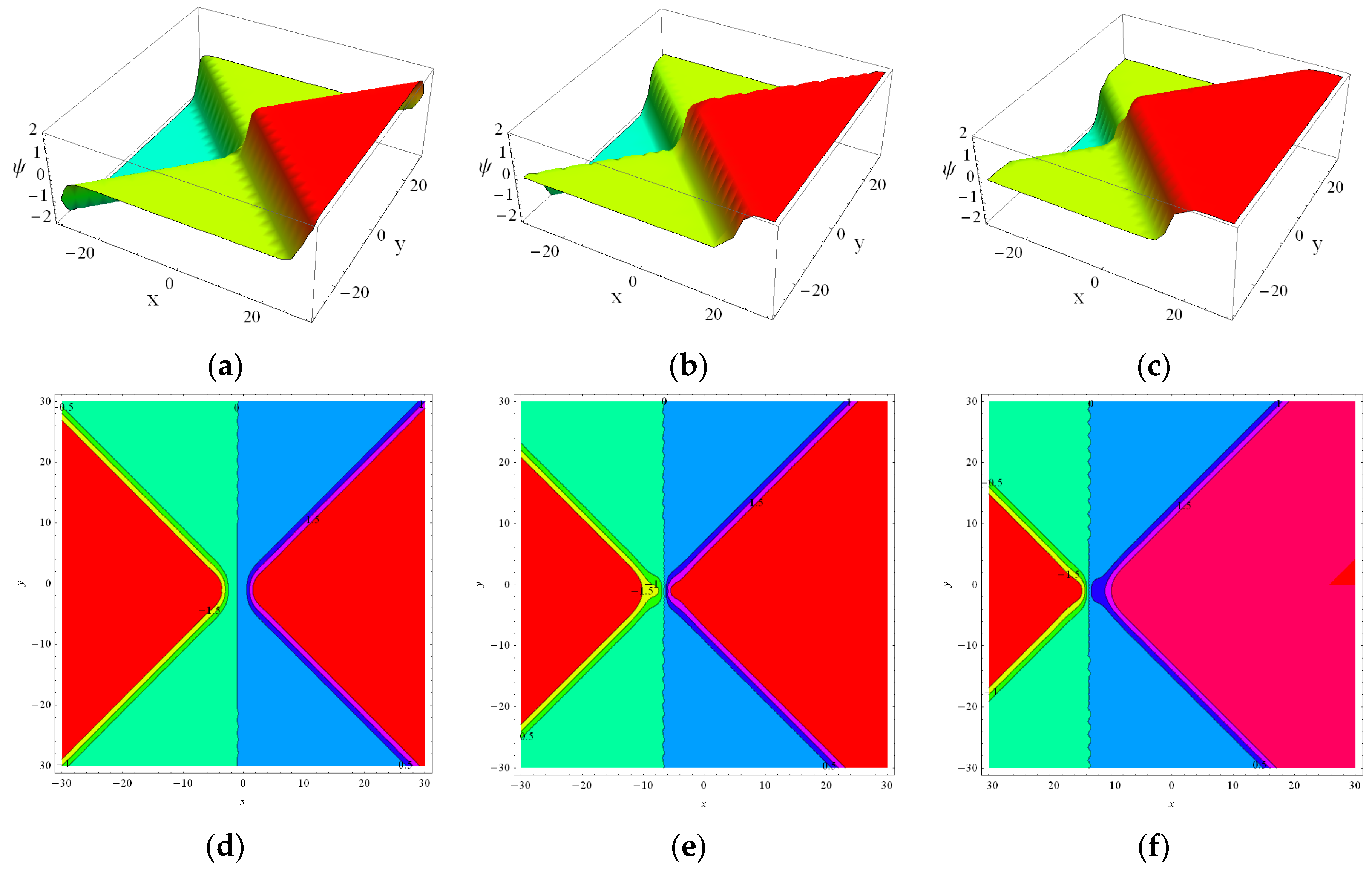
2.2. The Multi-Wave Solutions

To seek for the multi-wave solutions of Equation (1), we assume that g has the following form:
ϕ = ε 1 x + ε 2 y + ε 3 z + ε 4 t + ε 5 ,
φ = ε 6 x + ε 7 y + ε 8 z + ε 9 t + ε 10 ,
γ = ε 11 x + ε 12 y + ε 13 z + ε 14 t + ε 15 ,
g = Δ 1 cos ϕ + Δ 2 cos h φ + Δ 3 cos h γ + ε 16 ,
where ε i ( i = 1 , 2 , , 16 ) and Δ i ( i = 1 , 2 , 3 ) are real parameters to be determined later. Incorporating Equation (12) into Equation (3) yields a set of algebraic equations. Solving them, we have:
  • Case 1:
ε 1 = ε 1 ,   ε 2 = 0 ,   ε 3 = 0 ,   ε 4 = ε 4 ,   ε 5 = ε 5 ,   ε 6 = ε 6 ,   ε 7 = 0 ,   ε 8 = 0 ,   ε 9 = ε 6 ε 1 3 + ε 4 + ε 1 ε 6 2 ε 1 ,   ε 10 = ε 10 ,   ε 11 = 0 ,   ε 12 = ε 12 ,   ε 13 = ε 12 ε 1 3 + ε 4 3 ε 1 ,   ε 14 = 0 , ε 15 = ε 15 ,   ε 16 = ε 16 ,   Δ 1 = Δ 1 ,   Δ 2 = Δ 2 ,   Δ 3 = Δ 3 .
Substituting the above results into Equation (12) and adopting the transformation provided by Equation (2), we can obtain the multi-wave solution as:
ψ x , y , z , t = 2 ε 1 Δ 1 sin ε 1 x + ε 4 t + ε 5 + ε 6 Δ 2 sin h ε 6 x + ε 6 ε 1 3 + ε 4 + ε 1 ε 6 2 ε 1 t + ε 10 Δ 1 cos ε 1 x + ε 4 t + ε 5 + Δ 2 cos h ε 6 x + ε 6 ε 1 3 + ε 4 + ε 1 ε 6 2 ε 1 t + ε 10 + Δ 3 cos h ε 12 y ε 12 ε 1 3 + ε 4 3 ε 1 z + ε 15 + ε 16 .
  • Case 2:
ε 1 = ε 1 ,   ε 2 = ε 11 ε 12 ε 1 ,   ε 3 = ε 11 ε 12 4 ε 1 3 + ε 4 3 ε 1 2 ,   ε 4 = ε 4 ,   ε 5 = ε 5 ,   ε 6 = ε 6 ,   ε 7 = ε 11 ε 12 ε 6 ,   ε 8 = ε 11 ε 12 ε 1 3 + ε 4 3 ε 1 ε 6 2 3 ε 1 ε 6 ,   ε 9 = ε 6 ε 1 3 + ε 4 + ε 1 ε 6 2 ε 1 ,   ε 10 = ε 10 ,   ε 11 = ε 11 ,   ε 12 = ε 12 ,   ε 13 = ε 12 ε 1 3 3 ε 1 ε 11 2 + ε 4 3 ε 1 ,   ε 14 = ε 11 ε 1 3 + ε 1 ε 11 2 + ε 4 ε 1 ,   ε 15 = ε 15 ,   ε 16 = 0 , Δ 1 = Δ 1 ,   Δ 2 = Δ 2 ,   Δ 3 = Δ 3
Using the obtained results, we can obtain the multi-wave solution of Equation (1) by Equation (12) and Equation (2) as:
ψ ( x , y , z , t ) = 2 [ ε 1 Δ 1 sin ε 1 x ε 11 ε 12 ε 1 y + ε 11 ε 12 4 ε 1 3 + ε 4 3 ε 1 2 z + ε 4 t + ε 5 + ε 6 Δ 2 sinh ε 6 x + ε 11 ε 12 ε 6 y ε 11 ε 12 ε 1 3 + ε 4 3 ε 1 ε 6 2 3 ε 1 ε 6 z + ε 6 ε 1 3 + ε 4 + ε 1 ε 6 2 ε 1 t + ε 10 + ε 11 Δ 3 sinh ε 11 x + ε 12 y ε 12 ε 1 3 3 ε 1 ε 11 2 + ε 4 3 ε 1 z + ε 11 ε 1 3 + ε 1 ε 11 2 + ε 4 ε 1 t + ε 15 ] Δ 1 cos ε 1 x ε 11 ε 12 ε 1 y + ε 11 ε 12 4 ε 1 3 + ε 4 3 ε 1 2 z + ε 4 t + ε 5 + Δ 2 cosh ε 6 x + ε 11 ε 12 ε 6 y ε 11 ε 12 ε 1 3 + ε 4 3 ε 1 ε 6 2 3 ε 1 ε 6 z + ε 6 ε 1 3 + ε 4 + ε 1 ε 6 2 ε 1 t + ε 10 + Δ 3 cosh ε 11 x + ε 12 y ε 12 ε 1 3 3 ε 1 ε 11 2 + ε 4 3 ε 1 z + ε 11 ε 1 3 + ε 1 ε 11 2 + ε 4 ε 1 t + ε 15

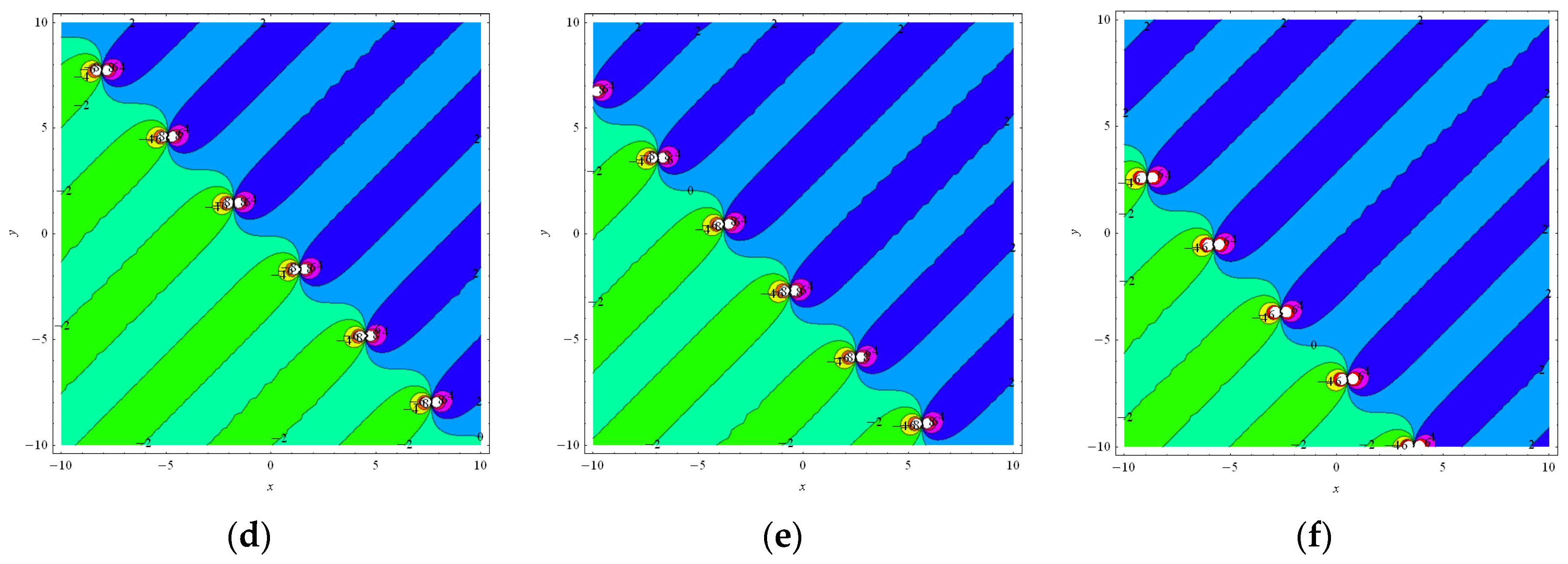
2.3. The Periodic Lump Solutions

To search for the periodic lump solutions of Equation (1). Here, the ansatz function g is supposed as the following form:
ϕ = x + ε 1 y + ε 2 z + ε 3 t ,
φ = x + ε 4 y + ε 5 z + ε 6 t ,
g = Δ 1 sin ϕ + Δ 2 cos h φ + ε 7 ,
where ε i ( i = 1 , 2 , , 7 ) and Δ i ( i = 1 , 2 ) are real parameters that can be determined later. In the same manner, substituting Equation (15) into Equation (3) and performing the corresponding adjustments, we have:
  • Case 1:
    ε 1 = ε 4 ,   ε 2 = ε 3 + 4 3 ,   ε 3 = ε 3 ,   ε 4 = ε 4 ,   ε 5 = 2 ε 4 ε 3 ε 4 3 ,   ε 6 = ε 3 + 2 ,   ε 7 = 0 ,   Δ 1 = Δ 1 ,   Δ 2 = Δ 2 .
Substituting the above results into Equation (15) and applying the transformation provided by Equation (2), we can obtain the periodic lump solution of Equation (1) as:
ψ x , y , z , t = 2 Δ 1 cos x ε 4 y + ε 3 + 4 3 z + ε 3 t + Δ 2 sin h x + ε 4 y + 2 ε 4 ε 3 ε 4 3 z + ε 3 + 2 t Δ 1 sin x ε 4 y + ε 3 + 4 3 z + ε 3 t + Δ 2 cos h x + ε 4 y + 2 ε 4 ε 3 ε 4 3 z + ε 3 + 2 t .
  • Case 2:
ε 1 = ε 1 ,   ε 2 = 2 ε 1 + ε 1 ε 6 3 ,   ε 3 = ε 6 2 ,   ε 4 = ε 1 ,   ε 5 = ε 1 ε 6 4 ε 1 3 ,   ε 6 = ε 6 ,   ε 7 = 0 ,   Δ 1 = Δ 1 ,   Δ 2 = Δ 2 .
Bringing the obtained results into Equation (15), we can obtain the periodic lump solution of Equation (1) with the help of the transformation provided by Equation (2) as:
ψ x , y , z , t = 2 Δ 1 cos x + ε 1 y 2 ε 1 + ε 1 ε 6 3 z + ε 6 2 t + Δ 2 sin h x ε 1 y + ε 1 ε 6 4 ε 1 3 z + ε 6 t Δ 1 sin x + ε 1 y 2 ε 1 + ε 1 ε 6 3 z + ε 6 2 t + Δ 2 cos h x ε 1 y + ε 1 ε 6 4 ε 1 3 z + ε 6 t .

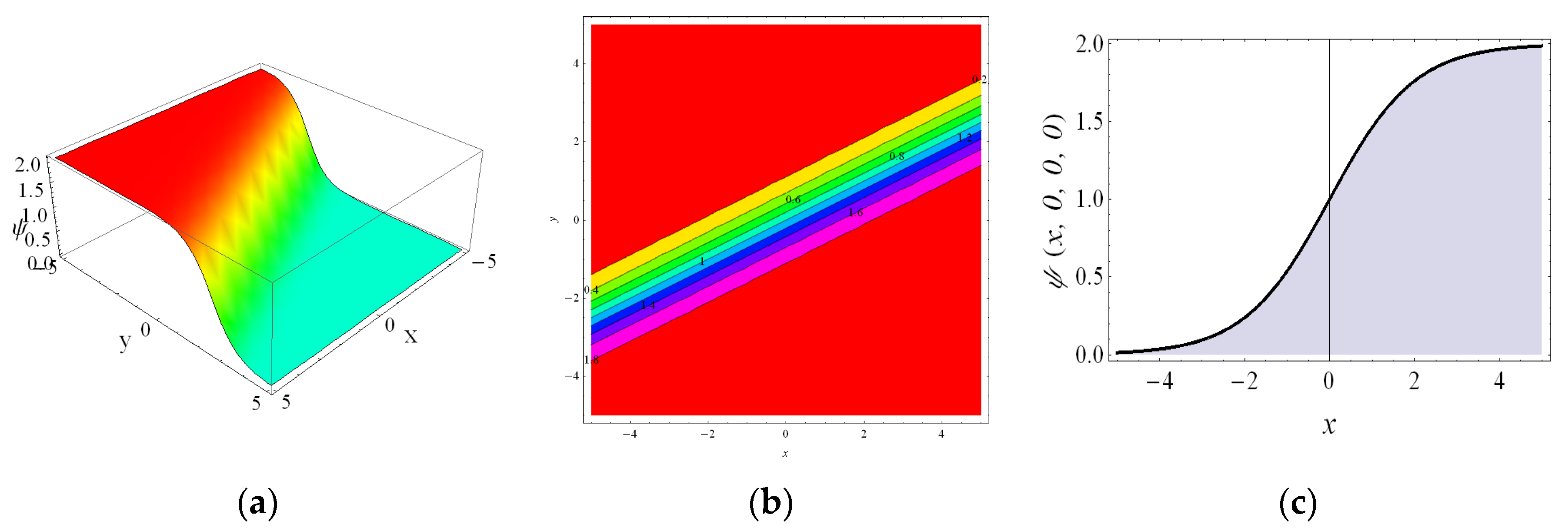
3. The Traveling Wave Solutions

In this section, we will inquire into the traveling wave solutions of Equation (1) with the aid of the sub-equation method [47,48].
To obtain the traveling wave solutions, we first introduce the following variable transformation:
ψ x , y , z , t = Ψ ζ ,   ζ = m x + n y + k z + s t ,
where m, n, k, s are non-zero constants. Putting it into Equation (1) yields:
m 3 n Ψ 4 + 3 m 2 n Ψ 2 n s + 3 m k Ψ = 0 ,
Integrating Equation (19) with respect to ζ once and ignoring the integral constant, we have:
m 3 n Ψ + 3 m 2 n Ψ 2 n s + 3 m k Ψ = 0 ,
Using the sub-equation method, we can assume the solution of Equation (20) is:
Ψ ζ = i = 0 c α i i ζ .
where α i i = 0 , 1 , 2 . , c are constants that can be determined later. Additionally, there is:
ζ = μ + 2 γ .
Here, μ is a constant. The solutions of Equation (22) are:
ζ = μ tan h μ ζ , μ < 0 μ cot h μ ζ , μ < 0 μ tan μ ζ , μ > 0 μ cot μ ζ , μ > 0 1 ζ + Λ , Λ i s a constant , μ = 0 .
By balancing Ψ and Ψ 2 in Equation (20), the value of c in Equation (21) can be determined as:
c = 1 .
Thus, we have:
Ψ ζ = α 0 + α 1 ζ .
Now, substituting Equation (25) with Equation (22) into Equation (20) and setting their coefficients of the different powers of ζ to be zero yields:
0 ζ : 3 k m μ α 1 n s μ α 1 + 2 m 3 n μ 2 α 1 + 3 m 2 n μ 2 α 1 2 = 0 ,
2 ζ : 3 k m α 1 n s α 1 + 8 m 3 n μ α 1 + 6 m 2 n μ α 1 2 = 0 ,
4 ζ : 6 m 3 n α 1 + 3 m 2 n α 1 2 = 0 .
On solving them, we have:
  • Case 1:
α 0 = α 0 ,   α 1 = α 1 ,   m = α 1 2 ,   n = n ,   k = k ,   s = α 1 3 k + n μ α 1 2 2 n ,   μ = μ .
So, the traveling wave solutions of Equation (1) can be obtained as:
ψ x , y , z , t = α 0 α 1 μ tan h μ α 1 2 x + n y + k z + α 1 3 k + n μ α 1 2 2 n t ,   μ < 0
ψ x , y , z , t = α 0 α 1 μ cot h μ α 1 2 x + n y + k z + α 1 3 k + n μ α 1 2 2 n t ,   μ < 0
ψ x , y , z , t = α 0 + α 1 μ tan μ α 1 2 x + n y + k z + α 1 3 k + n μ α 1 2 2 n t ,   μ > 0
ψ x , y , z , t = α 0 α 1 μ cot μ α 1 2 x + n y + k z + α 1 3 k + n μ α 1 2 2 n t ,   μ > 0
  • Case 2:
α 0 = α 0 ,   α 1 = 2 m ,   m = m ,   n = n ,   k = n s + 4 m 3 n μ 3 m ,   s = s ,   μ = μ .
So, the traveling wave solutions of Equation (1) can be obtained as:
ψ x , y , z , t = α 0 + 2 m μ tan h μ m x + n y n s + 4 m 3 n μ 3 m z + s t
ψ x , y , z , t = α 0 + 2 m μ cot h μ m x + n y n s + 4 m 3 n μ 3 m z + s t ,   μ < 0 .
ψ x , y , z , t = α 0 2 m μ tan μ m x + n y n s + 4 m 3 n μ 3 m z + s t ,   μ > 0 .
ψ x , y , z , t = α 0 + 2 m μ cot μ m x + n y n s + 4 m 3 n μ 3 m z + s t ,   μ > 0 .

4. The Numerical Results and Physical Interpretations

The numerical results will be presented by the 3-D plots, 2-D contours, and 2-D curves in this section by assigning the reasonable parameters with the help of the Mathematica software.
Figure 1 presents the behavior of the multi-waves complexiton solution provided by Equation (6) for using ε 2 = 2 , ε 9 = 3 , Δ 1 = 1 , Δ 2 = 1 , Δ 3 = 1 , Δ 4 = 1 for z = 0 at t = 0 , t = 4 and t = 8 in the form of a 3-D plot and 2-D contour. It can be observed that there were collision phenomena between the lump and singular periodic waves arising in the outline. As the time goes on, the wave is propagating along the negative direction of the x-axis and y-axis.
By assigning the parameters as ε 1 = 1 , ε 4 = 1 , ε 5 = 1 , ε 6 = 1 , ε 10 = 1 , ε 12 = 1 , ε 15 = 1 , ε 16 = 1 , Δ 1 = 1 , Δ 2 = 1 , and Δ 3 = 1 , we present the performance of Equation (13) in Figure 2 for z = 0 at t = 0 , t = 2 , and t = 4 through the 3-D plots and 2-D contours. We can find that the multi-wave is formed by the interleaving and superposition of two waveforms. As time goes on, one wave is propagating along the negative direction of x-axis and positive direction of y-axis, on the other hand, the other wave is propagating along the negative direction of the x-axis and y-axis.
Figure 3 presents the behaviors of Equation (16) by selecting the parameters as ε 3 = 1 , ε 4 = 1 , Δ 1 = 1 , and Δ 2 = 1 at z = 1 for t = 0 , t = 1 , and t = 2 via the 3-D plots and 2-D contours. It is easy to see the collision phenomena between the lump and singular periodic waves arising in the outline. With the increase in t , the waveform propagates along the negative direction of the x-axis and y-axis.
Assigning the parameters as α 0 = 1 , α 1 = 1 , n = 1 , k = 1 , and μ = 1 , the behaviors of Equation (26) and Equation (27) are described in Figure 4 and Figure 5, respectively. We can find the waveform of Equation (26) is the dark wave and of Equation (27) is the bright-dark wave.
If we choose the parameters as α 0 = 1 , m = 1 , n = 1 , s = 1 , and μ = 1 , we present the performances of Equation (28) and Equation (29) in Figure 6 and Figure 7, respectively. It can be observed that the profiles are both the singular periodic waves.

5. Conclusions and Future Recommendations

With the aid of the Cole—Hopf transform, we successfully constructed the multi-wave complexiton, multi-wave, and periodic-lump solutions of the (3+1)-dimensional B-type Kadomtsev—Petviashvili equation via applying the symbolic computation and the ansatz function schemes. Furthermore, we also find its abundant exact traveling solutions by means of the sub-equation method, which includes the dark wave, bright-dark wave, and singular periodic wave solutions. Finally, the numerical simulation of the solutions are presented through the 3-D plots, 2-D contours, and 2-D curves. Compared with the solutions reported in [35,36,37,38,39,40], it can be found that the diverse solutions in this work are all new, which can be used to extend the solutions of the (3+1)-dimensional B-type Kadomtsev—Petviashvili equation in fluid mechanics. The methods in this paper can be applied to study the exact solutions of the other PDEs in physics.
Recently, the fractal and fractional calculus have a wide range of applications in different fields [49,50,51,52,53,54,55,56,57]; how to apply them to Equation (1) is the direction of the future research.

Author Contributions

Conceptualization, K.-J.W.; methodology, K.-J.W.; writing—original draft preparation, K.-J.W.; writing—review and editing, J.-H.L.; data curation, J.S.; supervision, G.-D.W. All authors have read and agreed to the published version of the manuscript.

Funding

This work is supported by the Key Programs of Universities in Henan Province of China (22A140006), the Fundamental Research Funds for the Universities of Henan Province (NSFRF210324), Program of Henan Polytechnic University (B2018-40), the Innovative Scientists and Technicians Team of Henan Provincial High Education (21IRTSTHN016).

Data Availability Statement

The data that support the findings of this study are available from the corresponding author upon reasonable request.

Conflicts of Interest

The authors declare no conflict of interest.

References

  1. Jhangeer, A.; Hussain, A.; Junaid-U-Rehman, M.; Baleanu, D.; Riaz, M.B. Quasi-periodic, chaotic and travelling wave structures of modified Gardner equation. Chaos Solitons Fractals 2021, 143, 110578. [Google Scholar] [CrossRef]
  2. Wang, K.L. New perspective to the fractal Konopelchenko-Dubrovsky equations with M-truncated fractional derivative. Int. J. Geom. Methods Mod. Phys. 2023, 2023, 2350072. [Google Scholar] [CrossRef]
  3. Wang, K.J.; Si, J. On the non-differentiable exact solutions of the (2+1)-dimensional local fractional breaking soliton equation on Cantor sets. Math. Methods Appl. Sci. 2023, 46, 1456–1465. [Google Scholar] [CrossRef]
  4. Wang, K.L. Exact travelling wave solution for the local fractional Camassa-Holm-Kadomtsev-Petviashvili equation. Alex. Eng. J. 2022, 63, 371–376. [Google Scholar] [CrossRef]
  5. Yang, Z.; Cheng, D.; Cong, G.; Jin, D.; Borjalilou, V. Dual-phase-lag thermoelastic damping in nonlocal rectangular nanoplates. Waves Random Complex Media 2021, 1–20. [Google Scholar] [CrossRef]
  6. Wang, K.J.; Jing, S. Dynamic properties of the attachment oscillator arising in the nanophysics. Open Phys. 2023. [Google Scholar] [CrossRef]
  7. Ma, Y.X.; Tian, B.; Qu, Q.X.; Yang, D.-Y.; Chen, Y.-Q. Painlevé analysis, Bäcklund transformations and traveling-wave solutions for a (3+1)-dimensional generalized Kadomtsev-Petviashvili equation in a fluid. Int. J. Mod. Phys. B 2021, 35, 2150108. [Google Scholar] [CrossRef]
  8. Yin, Y.H.; Lü, X.; Ma, W.X. Bäcklund transformation, exact solutions and diverse interaction phenomena to a (3+1)-dimensional nonlinear evolution equation. Nonlinear Dyn. 2022, 108, 4181–4194. [Google Scholar] [CrossRef]
  9. Wang, K.J. Bäcklund transformation and diverse exact explicit solutions of the fractal combined KdV-mKdV equation. Fractals 2022, 30, 2250189. [Google Scholar] [CrossRef]
  10. Du, Z.; Tian, B.; Xie, X.Y.; Jun, C.; Wu, X.Y. Bäcklund transformation and soliton solutions in terms of the Wronskian for the Kadomtsev–Petviashvili-based system in fluid dynamics. Pramana 2018, 90, 45. [Google Scholar] [CrossRef]
  11. Ma, W.X. Lump solutions to the Kadomtsev-Petviashvili equation. Phys. Lett. A 2015, 379, 1975–1978. [Google Scholar] [CrossRef]
  12. Wang, K.J.; Liu, J.-H. Diverse optical soliton solutions to the Kundu-Mukherjee-Naskar equation via two novel techniques. Optik 2023, 273, 170403. [Google Scholar] [CrossRef]
  13. Wang, K.J. Diverse soliton solutions to the Fokas system via the Cole-Hopf transformation. Optik 2023, 272, 170250. [Google Scholar] [CrossRef]
  14. Zhang, Z.; Li, B.; Chen, J.; Guo, Q. Construction of higher-order smooth positons and breather positons via Hirota’s bilinear method. Nonlinear Dyn. 2021, 105, 2611–2618. [Google Scholar] [CrossRef]
  15. Wang, K.J. Variational principle and diverse wave structures of the modified Benjamin-Bona-Mahony equation arising in the optical illusions field. Axioms 2022, 11, 445. [Google Scholar] [CrossRef]
  16. Wang, K.J.; Shi, F.; Wang, G.D. Periodic wave structure of the fractal generalized fourth order Boussinesq equation travelling along the non-smooth boundary. Fractals 2022, 30, 2250168. [Google Scholar] [CrossRef]
  17. Mahak, N.; Akram, G. Extension of rational sine-cosine and rational sinh-cosh techniques to extract solutions for the perturbed NLSE with Kerr law nonlinearity. Eur. Phys. J. Plus 2019, 134, 1–10. [Google Scholar] [CrossRef]
  18. Wang, K.J.; Liu, J.-H.; Wu, J. Soliton solutions to the Fokas system arising in monomode optical fibers. Optik 2022, 251, 168319. [Google Scholar] [CrossRef]
  19. Rezazadeh, H.; Inc, M.; Baleanu, D. New solitary wave solutions for variants of (3+1)-dimensional Wazwaz-Benjamin-Bona-Mahony equations. Front. Phys. 2020, 8, 332. [Google Scholar] [CrossRef]
  20. Wang, K.J.; Liu, J.H. On abundant wave structures of the unsteady korteweg-de vries equation arising in shallow water. J. Ocean. Eng. Sci. 2022, in press. [Google Scholar] [CrossRef]
  21. Kudryashov, N.A. One method for finding exact solutions of nonlinear differential equations. Commun. Nonlinear Sci. Numer. Simul. 2012, 17, 2248–2253. [Google Scholar] [CrossRef] [Green Version]
  22. Alharbi, A.R.; Almatrafi, M.B.; Seadawy, A.R. Construction of the numerical and analytical wave solutions of the Joseph-Egri dynamical equation for the long waves in nonlinear dispersive systems. Int. J. Mod. Phys. B 2020, 34, 2050289. [Google Scholar] [CrossRef]
  23. Seadawy, A.R.; Kumar, D.; Chakrabarty, A.K. Dispersive optical soliton solutions for the hyperbolic and cubic-quintic nonlinear Schrödinger equations via the extended sinh-Gordon equation expansion method. Eur. Phys. J. Plus 2018, 133, 182. [Google Scholar] [CrossRef]
  24. Raza, N.; Arshed, S.; Sial, S. Optical solitons for coupled Fokas-Lenells equation in birefringence fibers. Mod. Phys. Lett. B 2019, 33, 1950317. [Google Scholar] [CrossRef]
  25. Afzal, U.; Raza, N.; Murtaza, I.G. On soliton solutions of time fractional form of Sawada-Kotera equation. Nonlinear Dyn. 2019, 95, 391–405. [Google Scholar] [CrossRef]
  26. Raza, N.; Javid, A. Optical dark and dark-singular soliton solutions of (1+ 2)-dimensional chiral nonlinear Schrodinger’s equation. Waves Random Complex Media 2019, 29, 496–508. [Google Scholar] [CrossRef]
  27. Wang, K.J.; Si, J. Optical solitons to the Radhakrishnan-Kundu-Lakshmanan equation by two effective approaches. Eur. Phys. J. Plus 2022, 137, 1016. [Google Scholar] [CrossRef]
  28. Zheng, B.; Wen, C. Exact solutions for fractional partial differential equations by a new fractional sub-equation method. Adv. Differ. Equ. 2013, 2013, 199. [Google Scholar] [CrossRef] [Green Version]
  29. Wang, K.J. A fractal modification of the unsteady korteweg-de vries model and its generalized fractal variational principle and diverse exact solutions. Fractals 2022, 30, 2250192. [Google Scholar] [CrossRef]
  30. Wang, K.J. A fast insight into the optical solitons of the generalized third-order nonlinear Schrödinger’s equation. Results Phys. 2022, 40, 105872. [Google Scholar] [CrossRef]
  31. Sağlam Özkan, Y.; Seadawy, A.R.; Yaşar, E. Multi-wave, breather and interaction solutions to (3+1) dimensional Vakhnenko-Parkes equation arising at propagation of high-frequency waves in a relaxing medium. J. Taibah Univ. Sci. 2021, 15, 666–678. [Google Scholar] [CrossRef]
  32. Seadawy, A.R.; Bilal, M.; Younis, M.; Rizvi, S.T.R.; Althobaiti, S.; Makhlouf, M.M. Analytical mathematical approaches for the double-chain model of DNA by a novel computational technique. Chaos Solitons Fractals 2021, 144, 110669. [Google Scholar] [CrossRef]
  33. Mohammed, W.W.; Albalahi, A.M.; Albadrani, S.; Aly, E.S.; Sidaoui, R.; Matouk, A.E. The Analytical Solutions of the Stochastic Fractional Kuramoto-Sivashinsky Equation by Using the Riccati Equation Method. Math. Probl. Eng. 2022, 2022, 5083784. [Google Scholar] [CrossRef]
  34. Al-Askar, F.M.; Mohammed, W.W.; Alshammari, M. Impact of brownian motion on the analytical solutions of the space-fractional stochastic approximate long water wave equation. Symmetry 2022, 14, 740. [Google Scholar] [CrossRef]
  35. Rizvi, S.T.R.; Seadawy, A.R.; Ali, I.; Bibi, I.; Younis, M. Chirp-free optical dromions for the presence of higher order spatio-temporal dispersions and absence of self-phase modulation in birefringent fibers. Mod. Phys. Lett. B 2020, 34, 2050399. [Google Scholar] [CrossRef]
  36. Ding, C.C.; Gao, Y.T.; Deng, G.F. Breather and hybrid solutions for a generalized (3+1)-dimensional B-type Kadomtsev-Petviashvili equation for the water waves. Nonlinear Dyn. 2019, 97, 2023–2040. [Google Scholar] [CrossRef]
  37. Abudiab, M.; Khalique, C.M. Exact solutions and conservation laws of a (3+ 1)-dimensional B-type Kadomtsev-Petviashvili equation. Adv. Differ. Equ. 2013, 2013, 1–7. [Google Scholar] [CrossRef] [Green Version]
  38. Huang, Z.R.; Tian, B.; Zhen, H.L.; Jiang, Y.; Wang, Y.P.; Sun, Y. Bäcklund transformations and soliton solutions for a (3+1)-dimensional B-type Kadomtsev-Petviashvili equation in fluid dynamics. Nonlinear Dyn. 2015, 80, 1–7. [Google Scholar] [CrossRef]
  39. Xu, Z.; Chen, H.; Dai, Z. Kink degeneracy and rogue potential solution for the (3+1)-dimensional B-type Kadomtsev-Petviashvili equation. Pramana 2016, 87, 31. [Google Scholar] [CrossRef]
  40. Cui, W.; Liu, Y.; Li, Z. Multiwave interaction solutions for a (3+1)-dimensional B-type Kadomtsev-Petviashvili equation in fluid dynamics. Int. J. Nonlinear Sci. Numer. Simul. 2021. [Google Scholar] [CrossRef]
  41. Ma, H.; Huang, H.; Deng, A. Soliton molecules and some novel hybrid solutions for (3+1)-dimensional B-type Kadomtsev-Petviashvili equation. Mod. Phys. Lett. B 2021, 35, 2150388. [Google Scholar] [CrossRef]
  42. Darvishi, M.T.; Najafi, M.; Arbabi, S.; Kavitha, L. Exact propagating multi-anti-kink soliton solutions of a (3+1)-dimensional B-type Kadomtsev-Petviashvili equation. Nonlinear Dyn. 2016, 83, 1453–1462. [Google Scholar] [CrossRef]
  43. Liu, J.G.; Zhu, W.H.; Osman, M.S.; Ma, W.-X. An explicit plethora of different classes of interactive lump solutions for an extension form of 3D-Jimbo-Miwa model. Eur. Phys. J. Plus 2020, 135, 412. [Google Scholar] [CrossRef]
  44. Lü, X.; Chen, S.-J. Interaction solutions to nonlinear partial differential equations via Hirota bilinear forms: One-lump-multi-stripe and one-lump-multi-soliton types. Nonlinear Dyn. 2021, 103, 947–977. [Google Scholar] [CrossRef]
  45. Lü, X.; Chen, S.-J. New general interaction solutions to the KPI equation via an optional decoupling condition approach. Commun. Nonlinear Sci. Numer. Simul. 2021, 103, 105939. [Google Scholar] [CrossRef]
  46. Ma, W.X. N-soliton solution and the Hirota condition of a (2+1)-dimensional combined equation. Math. Comput. Simul. 2021, 190, 270–279. [Google Scholar] [CrossRef]
  47. Akinyemi, L.; Şenol, M.; Iyiola, O.S. Exact solutions of the generalized multidimensional mathematical physics models via sub-equation method. Math. Comput. Simul. 2021, 182, 211–233. [Google Scholar] [CrossRef]
  48. Bekir, A.; Aksoy, E.; Cevikel, A.C. Exact solutions of nonlinear time fractional partial differential equations by sub-equation method. Math. Methods Appl. Sci. 2015, 38, 2779–2784. [Google Scholar] [CrossRef]
  49. Wang, K.J.; Liu, J.H. Periodic solution of the time-space fractional Sasa-Satsuma equation in the monomode optical fibers by the energy balance theory. EPL 2022, 138, 25002. [Google Scholar] [CrossRef]
  50. He, J.H.; He, C.H.; Saeed, T. A fractal modification of Chen-Lee-Liu equation and its fractal variational principle. Int. J. Mod. Phys. B 2021, 35, 2150214. [Google Scholar] [CrossRef]
  51. Wang, K.J.; Liu, J.H.; Si, J.; Shi, F. A new perspective on the exact solutions of the local fractional modified Benjamin-Bona-Mahony equation on Cantor sets. Fractal Fract. 2023, 7, 72. [Google Scholar] [CrossRef]
  52. He, J.H. Fractal calculus and its geometrical explanation. Results Phys. 2018, 10, 272–276. [Google Scholar] [CrossRef]
  53. Wang, K.J.; Zhu, H.W. Periodic wave solution of the Kundu-Mukherjee-Naskar equation in birefringent fibers via the Hamiltonian-based algorithm. EPL 2022, 139, 35002. [Google Scholar] [CrossRef]
  54. Yang, X.J.; Machado, J.A.T.; Cattani, C.; Gao, F. On a fractal LC-electric circuit modeled by local fract, On a fractal LC electric circuit modeled by local fractional calculus. Commun. Nonlinear Sci. Numer. Simul. 2017, 47, 200–206. [Google Scholar] [CrossRef]
  55. Wang, K.L. A novel variational approach to fractal Swift-Hohenberg model arising in fluid dynamics. Fractals 2022, 30, 2250156. [Google Scholar] [CrossRef]
  56. Baleanu, D.; Mohammadi, H.; Rezapour, S. Analysis of the model of HIV-1 infection of CD4+ T-cell with a new approach of fractional derivative. Adv. Differ. Equ. 2020, 2020, 71. [Google Scholar] [CrossRef] [Green Version]
  57. Wang, K.J. Exact traveling wave solutions to the local fractional (3+1)-dimensional Jimbo-Miwa equation on Cantor sets. Fractals 2022, 30, 2250102. [Google Scholar] [CrossRef]
Figure 1. The 3-D plots and 2-D contours of Equation (6) with the parameters as ε 2 = 2 , ε 9 = 3 , Δ 1 = 1 , Δ 2 = 1 , Δ 3 = 1 , and Δ 4 = 1 at z = 0 . (a,d) for t = 0 , (b,e) for t = 4 , (c,f), and for t = 8 .
Axioms 12 00095 g001
Figure 2. The 3-D plots and 2-D contours of Equation (13) with the parameters as ε 1 = 1 , ε 4 = 1 , ε 5 = 1 , ε 6 = 1 , ε 10 = 1 , ε 12 = 1 , ε 15 = 1 , ε 16 = 1 , Δ 1 = 1 , Δ 2 = 1 , and Δ 3 = 1 at z = 0 . (a,d) for t = 0 , (b,e) for t = 2 , and (c,f) for t = 4 .
Axioms 12 00095 g002
Figure 3. The 3-D plots and 2-D contours of Equation (16) with the parameters as ε 3 = 1 , ε 4 = 1 , Δ 1 = 1 , and Δ 2 = 1 at z = 1 . (a,d) for t = 0 , (b,e) for t = 1 , and (c,f) for t = 2 .
Axioms 12 00095 g003aAxioms 12 00095 g003b
Figure 4. The 3-D plots and 2-D curve of Equation (26) with the parameters as α 0 = 1 , α 1 = 1 , n = 1 , k = 1 , and μ = 1 . (a) 3-D plot for z = 0 and t = 0 , (b) 2-D contour for z = 0 and t = 0 , and (c) 2-D curve for y = 0 , z = 0 , and t = 0 .
Axioms 12 00095 g004
Figure 5. The 3-D plots and 2-D curve of Equation (27) with the parameters as α 0 = 1 , α 1 = 1 , n = 1 , k = 1 , and μ = 1 . (a) 3-D plot for z = 0 and t = 0 , (b) 2-D contour for z = 0 and t = 0 , and (c) 2-D curve for y = 0 , z = 0 , and t = 0 .
Axioms 12 00095 g005
Figure 6. The 3-D plots and 2-D contours of Equation (28) with the parameters as α 0 = 1 , α 1 = 1 , n = 1 , k = 1 , and μ = 1 . (a) 3-D plot for z = 0 and t = 0 , (b) 2-D contour for z = 0 and t = 0 , and (c) 2-D curve for y = 0 , z = 0 , and t = 0 .
Axioms 12 00095 g006
Figure 7. The 3-D plots and 2-D contours of Equation (29) with the parameters as α 0 = 1 , m = 1 , n = 1 , s = 1 , and μ = 1 . (a) 3-D plot for z = 0 and t = 0 , (b) 2-D contour for z = 0 and t = 0 , (c) 2-D curve for y = 0 , z = 0 , and t = 0 .
Axioms 12 00095 g007
Disclaimer/Publisher’s Note: The statements, opinions and data contained in all publications are solely those of the individual author(s) and contributor(s) and not of MDPI and/or the editor(s). MDPI and/or the editor(s) disclaim responsibility for any injury to people or property resulting from any ideas, methods, instructions or products referred to in the content.

