Article

Inferences of a Mixture Bivariate Alpha Power Exponential Model with Engineering Application

1
Department of Mathematical Sciences, College of Science, Princess Nourah bint Abdulrahman University, P.O. Box 84428, Riyadh 11671, Saudi Arabia
2
Faculty of Science, King Abdulaziz University, Jeddah 21589, Saudi Arabia
3
Department of Statistics, Faculty of Commerce, Zagazig University, Zagazig 44519, Egypt
4
Department of Mathematics and Statistics, University of North Carolina, Wilmington, NC 28403, USA
5
Department of Statistics, Al-Azhar University, Cairo 11651, Egypt
6
Faculty of Technology and Development, Zagazig University, Zagazig 44519, Egypt
*
Author to whom correspondence should be addressed.
Axioms 2022, 11(9), 459; https://doi.org/10.3390/axioms11090459
Submission received: 8 August 2022 / Revised: 2 September 2022 / Accepted: 4 September 2022 / Published: 7 September 2022
(This article belongs to the Special Issue Computational Statistics & Data Analysis)

Abstract

:
The univariate alpha power exponential (APE) distribution has several appealing characteristics. It behaves similarly to Weibull, Gamma, and generalized exponential distributions with two parameters. In this paper, we consider different bivariate mixture models starting with two independent univariate APE models, and, in the latter case, starting from two dependent APE models. Several useful structural properties of such a mixture model (under the assumption of two independent APE distribution) are discussed. Bivariate APE (BAPE), in short, modelled under the dependent set up are also discussed in the context of a copula-based construction. Inferential aspects under the classical and under the Bayesian paradigm are considered to estimate the model parameters, and a simulation study is conducted for this purpose. For illustrative purposes, a well-known motor data is re-analyzed to exhibit the flexibility of the proposed bivariate mixture model.

1. Introduction

Univariate continuous alpha power exponential distribution with two parameters has received a considerable amount of attention among researchers working in the area of distribution theory. Since the introduction of the model, an appreciable amount of work has taken place on the development of bivariate APE distribution and its different generalizations; for more information, see Ref. [1] and the references cited therein. In this paper, we discuss several different bivariate APE models with various mixing mechanisms. Noticeably, mixture distribution plays an important role in various data-analysis purposes; see [2]. Precisely, if the data are coming from different subpopulations, and their identifications are unknown, then the mixture distribution can be used quite effectively to analyze the data set. Unlike any other symmetric distribution (for example, normal) APE distribution is a skewed distribution. Consequently, if the subpopulations do not have symmetric distribution, the mixture of APE resulting in a bivariate APE distribution may be used to analyze these data. Furthermore, a multi-model distribution can be well approximated by a mixture distribution. Not much work has been carried out on a bivariate mixture of APE distribution.
This is an effort towards that direction. We consider two different mixing strategies to construct the bivariate mixture APE (BMAPE type I). In both cases, we start with the following: let X ~ A P E α 1 ,   θ 1 and Y ~ A P E α 2 ,   θ 2 , and let them be independent. In the first, we consider a finite mixing strategy as described above and call it a BMAPE distribution. While, in the second scenario, we consider a copula-based construction approach. We consider a bivariate Gaussian copula to construct a copula-based bivariate distribution which we call (henceforth) BMAPE (type I). One of the major objectives for a copula-based construction is that we can better discuss the dependence structure between two components. For a copula-based bivariate and multivariate distribution, see [3]. In the next, we provide a non-exhaustive list of pertinent references that serves as motivation to carry out the present work.
Statisticians and practitioners have been particularly interested in studying groups that demonstrate similar behavior in response to pre-determined criteria. Refs. [4,5] developed and utilized a method known as finite mixture distributions, and provided the majority of the early evidence for the study of heterogeneous populations as a possible application of finite mixture models. Studies focusing on heterogeneous populations became more popular in the modern era as data-related computation facilities improved. For some useful references, see [6,7,8,9,10] and the references cited therein. Starting with one parameter exponential baseline distribution, Ref. [1] developed the alpha power exponential (APE) distribution, discussed its several useful properties, and studied the associated statistical inference. Ref. [11] introduced the alpha power Weibull distribution and demonstrated that it provides superior modelling to several other generalizations of the Weibull distribution, in particular, when modeling heterogenous population. To introduce the alpha power generalized exponential (APGE) distribution, Ref. [12] employed the generalized exponential baseline distribution and the alpha power transformation (APT) technique. Ref. [13] developed closed-form expressions for the alpha power generalized exponential (APGE) distribution’s moment properties. Ref. [14] presented a new family of APT-based distributions by inverting the quantile function of any distribution as a function of the APT cumulative distribution function (CDF). In the next, we provide a non-exhaustive list of references related to APT-based mixture distributions that are developed in the univariate domain. The alpha power exponentiated Weibull distribution was suggested by Ref. [3], who investigated the general mathematical features of the APT family. Ref. [15] introduced the Marshall Olkin alpha power family as a new generalization of the APT and a novel approach to studying the mathematical properties of the APT model was introduced by Ref. [16]. The probability density function (PDF) and the hazard functions of the APE distribution are similar to those of the Weibull, Gamma, and generalized exponential (GE) distributions under certain specific choices of the model parameters. As a result, it can be used as a variable alternative for the widely used Weibull, Gamma, and GE distributions. Specially, when, component-wise, each one of them cannot provide best fit, such a mixture mode will be a good fit. As the CDF of the APE distribution has a closed form which is analytically tractable, it can be used to analyze censored data sets as well.
Mixture distributions are made up of a finite or an infinite number of components, which may be comprised of several different distributions, and can be used to represent various aspects of data for example, two of the most notable studies that explore different sorts of combinations of distributions can be found in Refs. [17,18]. Discussion on a finite three-component mixture of exponential distribution can be found in Ref. [19]. In the literature, there are not many references of finite and/or infinite mixtures of probability models. A non-exhaustive list of references can be cited as follows. A mixture of bivariate exponential distributions (MBE), in which the authors predicted the elements of MBE are given in Ref. [20]. Discussion on a new bivariate distribution whose both marginals are finite mixtures of gamma distribution are nicely explored in Ref. [21]. For a review of known bivariate distributions, we refer the readers to Refs. [22,23,24]. The univariate exponential distribution is one of the most celebrated distributions because of its importance in many lifetime applications and its structural properties. Consequently, if we consider a simple bivariate expansion, there might be limitations due to properties, especially for modeling heterogenous data. This motivates us to consider a mixture form that will have many desirable properties. In this article, we propose and study a finite mixture of a bivariate continuous probability model arising from two independent univariate APE distributions, which we call BMAPE, in short. In this paper, we consider various mechanisms of mixing univariate APE distributions to construct a bivariate mixture of APE models, which are listed below:
(i)
In the first case, we start with two independent and univariate APE with parameters α 1 , α 2 ,   θ and μ 1 ,   μ 2 , λ with α 1 α 2 , μ 1   μ 2 . Further, we assume that α 1 , α 2 ,   μ 1 ,   μ 2 are random variables. Then, using the methodology of compounding, we develop the bivariate APE distribution, and, for the sake of notational simplicity, call it the BMAPE (type-I) distribution.
(ii)
In the second scenario, we consider a copula-based construction approach. We consider a bivariate Gaussian copula in which the margins are two univariate and independent APE distributions with the coupling parameter ρ . For notational simplicity, we call this the BMAPE (type-II) distribution, for more details of copula based on construction and associated properties, see [25].
The remainder of the paper is laid out as follows. In Section 2, we describe the BMAPE (type-I) distribution and discuss its properties. In Section 3, we provide some useful properties of the BMAPE (type-I) distribution, including the survival function, hazard rate function and conditional moments. In Section 4, we look at how the expectation-maximization (EM) technique can be used to estimate model parameters for BMAPE (type-I) distribution. The estimation approach for the BMAPE (type-II) distribution formed using the bivariate Gaussian copula is discussed in Section 5. In Section 6, we investigate how to estimate model parameters under the Bayesian paradigm. In Section 7, the simulation results are reported. A well-known Motor data set was re-analyzed in Section 8 to demonstrate the efficacy of the suggested BMAPE type models. Finally, in Section 9, we wrap up the paper with some concluding remarks.

2. The APE Model with a Bivariate Mixture

We will start with two independent univariate APE distributions with parameters of α ,   θ and μ , λ , respectively. We employ here the strategy of compounding by assuming that α and μ are random variables; then, the marginal joint distribution of X i n and Y i n may be derived from the joint distribution of α and μ respectively, which is given as follows
h 1 x , y x , y = h 1 x , y , α , μ d α   d μ ,  
where X i n and Y i n are independent APE distributions. Next, we consider two different scenarios in the context of the nature of the distributions of X i n and Y i n . From (1), one may obtain the desired BMAPE (type-I) distribution.
We generate a bivariate mixture of the APE distribution in two scenarios. In the first scenario, X i n and Y i n are independent APE distributions with a generalized bivariate Bernoulli distribution for the shape parameters as
μ 1 μ 2 P = α 1 α 2 P α 1 μ 1 P α 1 μ 2 P α 2 μ 1 P α 2 μ 2 .
A random variable with an APE distribution has a CDF and a PDF for X i n > 0 , given by, respectively,
F x i n , α , θ = α 1 e θ x i n 1 α 1 ,   x i n > 0 ,   θ   α > 0 ,   i = 1 , 2 ,  
f x i n , α , θ = θ l o g α e θ x i n α 1 e θ x i n α 1 ,   x i n > 0 ,
where α and θ are the shape and scale parameters.
Next, in order to construct a finite mixture of bivariate alpha power exponential model, we proceed as follows:
(i)
We consider X i ~ A P E   α i , θ   i = 1 , 2 ,   where   α 1 and α 2 are random and θ is fixed, and each are independent for fixed choices of α 1 and α 2 . Likewise, Y i ~ A P E   μ i , λ   i = 1 , 2 , where μ 1 and μ 2 are random and λ is fixed.
(ii)
Next, we further assume that X 1 , X 2   and   Y 1 , Y 2 are independent but α i   , μ i ,   i = 1 , 2 , are correlated through their bivariate generalized Bernoulli distribution with the shape parameter α i   , μ i , assuming the following probability matrix.
μ 1 μ 2 P = α 1 α 2 P α 1 μ 1 P α 1 μ 2 P α 2 μ 1 P α 2 μ 2 ,
where P is the mixing component with the condition i = 1 2 P α i μ i = 1 .
Let h 1 x , y be the joint PDF created from the marginal densities of x i   , y i ,   i = 1 , 2 ,   given   earlier .
Then, the joint density of x , y can be written as
h 1 x , y x , y = f ( x 1 | α 1 , θ ) g y 1 | μ 1 , λ P α 1 μ 1 + f ( x 2 | α 1 , θ ) g y 2 | μ 2 , λ P α 1 μ 2 + f ( x 2 | α 2 , θ ) g y 1 | μ 1 , λ P α 2 μ 1 + f ( x 2 | α 2 , θ ) g y 2 | μ 2 , λ P α 2 μ 2 ,
Then,
h 1 x , y = P α 1 μ 1 θ l o g α 1 e θ x 1 α 1 1 e θ x 1 α 1 1 × λ l o g μ 1 e λ y 1 μ 1 1 e λ y 1 μ 1 1 + P α 1 μ 2 θ l o g α 1 e θ x 1 α 1 1 e θ x 1 α 1 1 × λ l o g μ 2 e λ y 2 μ 2 1 e λ y 2 μ 2 1 + P α 2 μ 1 θ l o g α 2 e θ x 2 α 2 1 e θ x 2 α 2 1 × λ l o g μ 1 e λ y μ 1 1 e λ y μ 1 1 + P α 2 μ 2 θ l o g α 2 e θ x 2 α 2 1 e θ x 2 α 2 1 × λ l o g μ 2 e λ y 2 μ 2 1 e λ y 2 μ 2 1 ,   x i > 0 , y i > 0 .
For this model, it appears that, for a valid PDF, we must have this constraint α , μ > 0 and α , μ 1 .
To make things easier in terms of writing and visualization, let a = P α 1 μ 1 , b = P α 1 μ 2 , c = P α 2 μ 1 and d = P α 2 μ 2 . Depending on a variety of choices for the mixing parameters a ,   b ,   c ,   d ,   θ ,   λ ,   α i and μ i for i = 1 , 2 , several shapes of the joint PDF in (5) are provided in Figure 1. Moreover, several contour plots for various values of a , b , c and d when α 1 , α 2 , μ 1 , μ 2 , θ , λ = 9 , 7 , 6 , 5 , 1.2 , 0.6 are displayed in Figure 2. As one might expect, not all four components may be required in applications to real-world data sets. Consequently, some constraints can be applied, such as b = c = 0 , a = d = 0 or a = b = c = 0 , as appropriate. These constraints result in correlation values of +1, −1, and 0 among the shape parameter, respectively.
The marginal densities of X and Y, respectively, from the joint PDF in (5) are not available in closed form; one may consider some numerical methods to obtain an approximate expression. The CDF for the joint model will be
F x , y = 0 y 0 x h 1 t , s d t   d s = 0 y 0 x [ a θ l o g α 1 e θ t α 1 1 e θ t α 1 1 × λ l o g μ 1 e λ s μ 1 1 e λ s μ 1 1 + b θ l o g α 1 e θ t α 1 1 e θ t α 1 1 × λ l o g μ 2 e λ s μ 2 1 e λ s μ 2 1 + c θ l o g α 2 e θ t α 2 1 e θ t α 2 1 × λ l o g μ 1 e λ s μ 1 1 e λ s μ 1 1 + d θ l o g α 2 e θ t α 2 1 e θ t   α 2 1 × λ l o g μ 2 e λ s μ 2 1 e λ s μ 2 1 ] d t d s    = a α 1 1 e θ x 1 μ 1 1 e λ y 1 α 1 1 μ 1 1 + b α 1 1 e θ x 1 μ 2 1 e λ y 1 α 1 1 μ 2 1 + c α 2 1 e θ x 1 μ 1 1 e λ y 1 α 2 1 μ 1 1 + d α 2 1 e θ x 1 μ 2 1 e λ y 1 α 2 1 μ 2 1 .
For (6), to be a valid CDF, we must have
(i)
F x , y 0 ,   x , y + α 1 ,   μ 1 ,   α 2 ,   μ 2 > 0 and α 1 ,   μ 1 ,   α 2 ,   μ 2 0 .
(ii)
l i m x , y 0 F x , y = 0 .
(iii)
l i m x , y F x , y = 1 .
Next, one may obtain the marginal survival functions for the smallest order statistics for a random sample of size two. For example, let w 1 = m i n X , Y , then, F ¯ W 1 w 1 = P m i n X , Y > w 1 = P X > w 1 , Y > w 1 , while
F ¯ W 2 W 2 = P m a x X , Y < w 2 = P X w 2 , Y w 2
From (7), one can obtain the associated PDF for W 2 . We discuss some useful structural properties in the next section for the BMAPE (type-I) distribution.

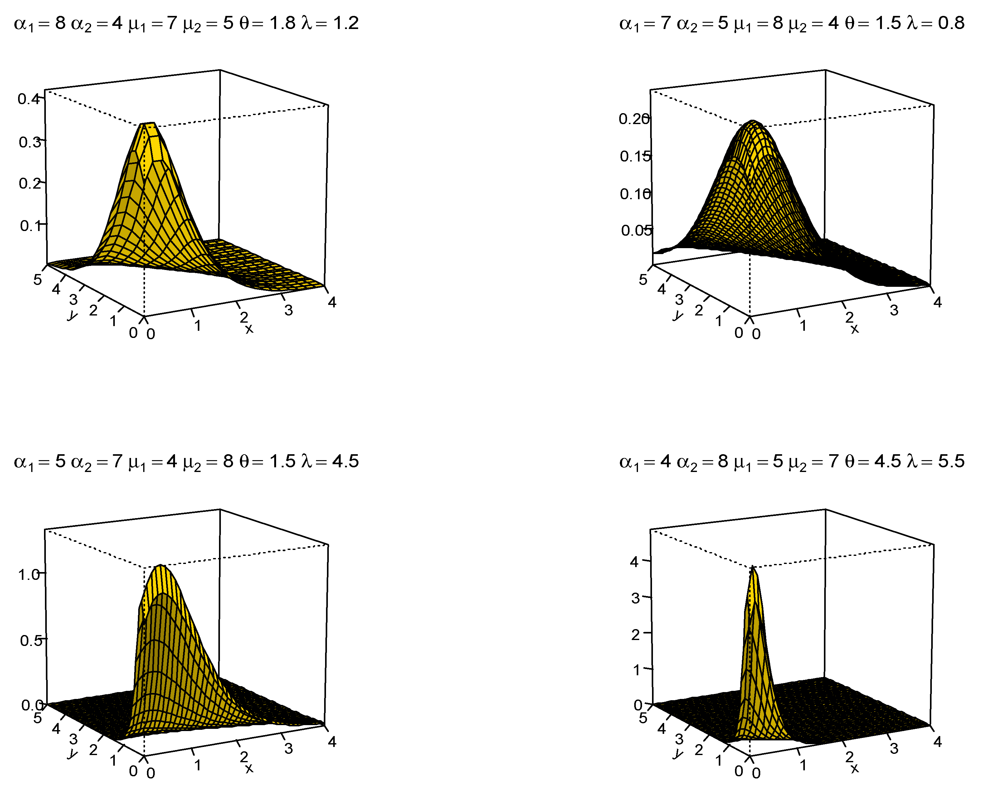
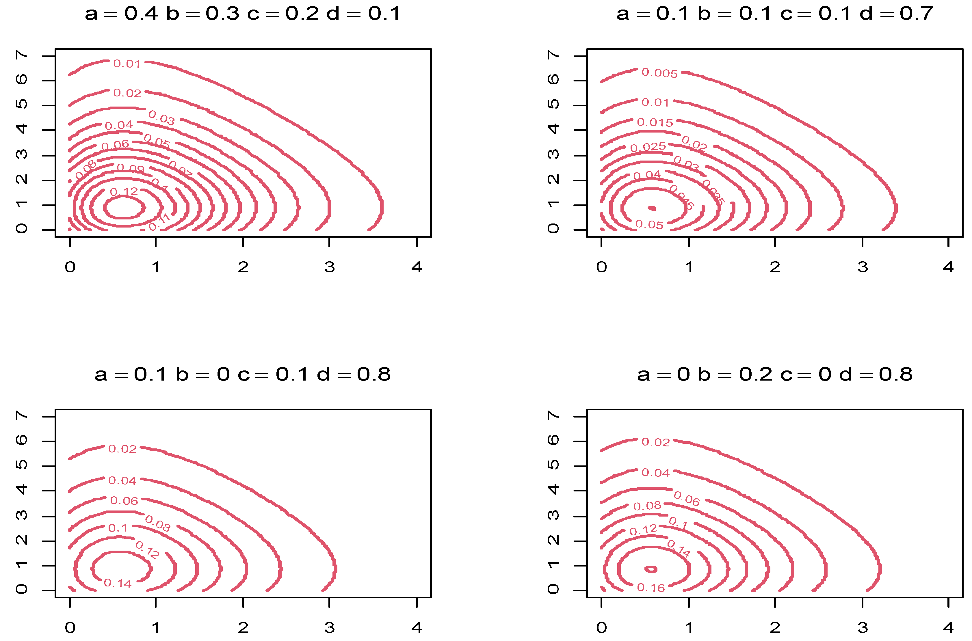
3. Structural Properties

Theorem: The BMAPE (type I) distribution is log-concave. Taking the negative logarithm of (5), for 0 < x < y < (or for 0 < y < x < ), we obtain
l o g h 1 x , y = l o g P α 1 μ 1 θ l o g α 1 e θ x α 1 1 e θ x α 1 1 × λ l o g μ 1 e λ y μ 1 1 e λ y μ 1 1 + P α 1 μ 2 θ l o g α 1 e θ x α 1 1 e θ x α 1 1 × λ l o g μ 2 e λ y μ 2 1 e λ y μ 2 1 + P α 2 μ 1 θ l o g α 2 e θ x α 2 1 e θ x α 2 1 × λ l o g μ 1 e λ y μ 1 1 e λ y μ 1 1 + P α 2 μ 2 θ l o g α 2 e θ x α 2 1 e θ x α 2 1 × λ l o g μ 2 e λ y μ 2 1 e λ y μ 2 1   .
Next, taking partial derivatives w.r.t. x and y of (8), respectively, we obtain
D y D x l o g h 1 x , y = P α 1 μ 2 P α 2 μ 1 P α 1 μ 1 P α 2 μ 2 e θ x λ y θ λ α 1 1 α 1 e θ x + 1 α 2 1 α 2 e θ x + 1 × μ 1 1 μ 2 1 μ 1 1 + e λ y μ 2 1 + e λ y l o g α 1 l o g α 1 l o g α 2 l o g α 2 l o g α 1 l o g μ 1 l o g μ 2 × α 1 α 2 1 α 2 e θ x l o g α 1 P α 1 μ 1 μ 1 l o g μ 1 μ 2 1 μ 2 e λ y + P α 1 μ 2 μ 2 l o g μ 2 μ 1 1 μ 1 e λ y × + α 1 1 α 1 e θ x α 2 l o g α 2 P α 2 μ 1 μ 1 l o g μ 1 μ 2 1 μ 2 e λ y + P α 2 μ 2 μ 2 l o g μ 2 μ 1 1 μ 1 e λ y 2 .
It is obvious from (9) that, provided α 1 > 1 ,   μ 1 > 1 ,   α 2 > 1 ,   μ 2 > 1 , the expression in (9) is greater than zero with the assumption that P α 1 μ 2 P α 2 μ 1 > P α 1 μ 1 P α 2 μ 2 , i.e., the joint density in (5) is log-concave.
The BMAPE (type-I) distribution’s survival function will be
R x , y = P X > x , Y > y = 1 P X < x P Y < y + P X < x , Y < y = 1 F X x F Y y + F X , Y x , y
The marginal distribution functions of X and Y are F X x and F Y y , respectively. The following is the hazard rate function (hrf):
h r f x , y = 1 F X x F Y y + F X , Y x , y 1 × a θ l o g α 1 e θ x α 1 1 e θ x α 1 1 × λ l o g μ 1 e λ y μ 1 1 e λ y μ 1 1 + b θ l o g α 1 e θ x α 1 1 e θ x α 1 1 × λ l o g μ 2 e λ y μ 2 1 e λ y μ 2 1 + c θ l o g α 2 e θ x α 2 1 e θ x α 2 1 × λ l o g μ 1 e λ y μ 1 1 e λ y μ 1 1 + d θ l o g α 2 e θ x α 2 1 e θ x α 2 1 × λ l o g μ 2 e λ y μ 2 1 e λ y μ 2 1 .
For each fixed Y = y, the conditional PDF of X given Y as well as Y given X are given, respectively, by
f x y = h 1 x , y h 1 y y   and   f y x = h 1 x , y h 1 x x .
Proposition 1. 
Let X ,   Y ~ B M A P E   t y p e   I   a , b , c , d , α 1 , α 2 , μ 1 , μ 2 , θ ,   λ . Then, (X,Y) has a positive association with a total positivity of order 2 ( T P 2 ), provided ( α 1 , α 2 , μ 1 , μ 2 ) > 1 . Observe that an absolute continuous bivariate random vector, such as U 1 ,   U 2 , has the T P 2 property if and only if for each u 11 , u 12 ,   u 21 ,   a n d   u 22 , whenever u 11 < u 12 and u 21 > u 22 , it satisfies f U 1 ,   U 2 u 11 ,   u 21 f U 1 ,   U 2 u 11 ,   u 12 f U 1 , U 2 u 12 ,   u 21 f U 1 ,   U 2 u 11 ,   u 22 0 , where f U 1 ,   U 2 u 1 ,   u 2 is the joint PDF. Take distinct ordered u 11 , u 12 ,   u 21 and u 22 such that u 11 < u 12 and u 21 > u 22 , and our result follows instantly. Consequently, the positive quadrant dependence property (also known as the T P 2 property) would reveal a number of non-increasing features relating to conditional survival, the conditional CDF of X given Y, and Y given X, as well as the following finding: g 1 . and g 2 . , C o v g 1 X ,   g 2 Y   0 .
Proposition 2. 
Shape of the distribution
A critical point in a two-variable function is where the first-order partial derivatives are equal to zero. The following are the two most compelling reasons to investigate the critical points of a bivariate distribution:
(1)
A real-life data set (or sets) can assume a variety of shapes. A study such as this can help determine the adaptability of this bivariate distribution.
(2)
When working with bivariate distributions, it is essential to examine the joint PDF’s tails as well as the point of inflection. This study is useful in the context of data fitting, as data sets having heavier tails and/or which are small can be adequately modeled by a distribution exhibiting one of these features, as appropriate. Critical-point(s) knowledge will aid in a better understanding of these features, as will be illustrated in Appendix A.

4. Inference

In this section, we consider the estimation of the model parameters of the BMAPE (type-I) distribution using the EM algorithm. The EM algorithm, originally proposed by [2], is an iterative approach for determining the maximum likelihood estimator of a parameter in a parametric probability distribution. To use the EM technique, we combine the data ( x k ,   y k ) ,   k = 1 , ,   n (to be obtained from a random sample of size n obtained from the associated joint density) with the group membership variables Φ k = a k , b k , c k , k = 1 , , n , where a k is an indicator variable that is one if the k t h observation is in f x , α 1 ,   μ 1 and zero otherwise. Similarly, we have four groups f i j ,   i , j = 1 ,   2 , for b k , c k , with the following densities of
f i j x , y = f i x f j y = θ 1 l o g α e θ 1 x α 1 e θ 1 x α 1   λ 1 l o g μ e λ 1 y μ 1 e λ 1 y μ 1 ,
where P f 11 = a , P f 12 = b , P f 21 = c , and P f 22 = 1 a b c are the equivalent mixing proportions.
The associated log likelihood function for the complete sample i j x , y = l o g f i j x , y , is symbolized by:
= k = 1 n a k 11 x k ,   y k + k = 1 n b k 12 x k ,   y k + k = 1 n c k 21 x k ,   y k + k = 1 n 1 a k b k c k 22 x k ,   y k .
The EM method has two steps: Step-E (expectation) and Step-M (maximization) in each iteration. As the group membership variables represented as Φ k are linear, we replace the related expected values in (11) with the current estimates ( α ^ 1 ,   μ ^ 1 , α ^ 2 ,   μ ^ 2 ,   λ ^ , θ ^ , a ^ , b ^ , c ^ ) of the parameters determined and, subsequently, an update occurs. For more information on this topic, see [26] as:
a ^ k = a ^ f 11 x k ,   y k a ^ f 11 x k ,   y k + b ^ f 12 x k ,   y k + c ^ f 21 x k ,   y k + 1 a ^ b ^ c ^   f 22   x k   , y k .
Similarly, for b k and c k , apply the same technique, as follows:
b ^ k   = b ^ f 12 x k ,   y k a ^ f 11 x k ,   y k + b ^ f 12 x k ,   y k + c ^ f 21 x k ,   y k + 1 a ^ b ^ c ^   f 22   x k   , y k   and   c ^ k   = c ^ f 21 x k ,   y k a ^ f 11 x k ,   y k + b ^ f 12 x k ,   y k + c ^ f 21 x k ,   y k + 1 a ^ b ^ c ^   f 22   x k   , y k .
Following that, in the M-step, we maximize (11) across λ , θ , α 1 , α 2 , μ 1 , μ 2 for fixed values of Φ k . The conditional independence of X and Y given the group membership achieves maximization by differentiating (11), which are:
ι α 1 = n α 1 1 k = 1 n a k + b k + n α 1 log α 1 k = 1 n a k + b k + 1 α 1 k = 1 n a k + b k 1 e θ x ,
ι μ 1 = n μ 1 1 k = 1 n a k + c k + n μ 1 log μ 1 k = 1 n a k + c k + 1 μ 1 k = 1 n a k + c k 1 e λ y ,  
ι α 2 = n α 2 1 k = 1 n c k + d k + n α 1 log α 1 k = 1 n c k + d k + 1 α 1 k = 1 n c k + d k 1 e θ x ,
ι μ 2 = n μ 2 1 k = 1 n b k + d k + n μ 2 log μ 2 k = 1 n b k + d k + 1 μ 1 k = 1 n b k + c k 1 e λ y ,  
ι θ = n θ k = 1 n a k + b k + c k + d k k = 1 n a k + b k + c k + d k x k l o g α 1 k = 1 n x k a k + b k e θ x k l o g α 2 k = 1 n x k c k + d k e θ x k ,  
and
ι λ = n λ k = 1 n a k + b k + c k + d k k = 1 n a k + b k + c k + d k y k l o g μ 1 k = 1 n y k a k + c k e λ y k l o g μ 2 k = 1 n y k b k + d k e λ y k .
The M-step is then completed by setting
a ^ = n 1 k = 1 n a k ,   etc .  
The model parameters must have a starting value to initiate the process, which is denoted by the symbol Φ 0 . To ensure that the proposed EM algorithm’s rate of convergence does not become significantly sluggish, careful selection of these initial values is required. Another factor to consider is that the maximum likelihood equation may have several solutions corresponding to local maxima, necessitating careful selection of starting values. In the literature, some discussion on the identification of starting value(s) have been discussed and the references cited therein. The “coda” and “maxLik” of R package were used to quantitatively solve these equations. After obtaining the maximum likelihood estimators (MLEs) for α 1 , μ 1 , α 2 , μ 2 , θ , λ ,   δ , ρ 11 , ρ 12 ,   ρ 21 and ρ 22 , we replace these estimates in ( a k ,   b k ,   c k ). Then, the M-step is completed by setting a ^ = n 1 k = 1 n a k , and the process continues. To produce initial values for the mixing proportions individually, the matching moment’s method for the marginal univariate APE parameter is employed. The BMAPE (type-I) parameter estimates are used as the starting points for the EM technique. Then, assuming that the two variables X and Y are independent, we combine the marginal mixing parameter moment estimators to obtain initial values for the bivariate mixing parameters. Specific details are provided in Section 7, and, more specifically, in Tables 2–4. By assuming that the two variables X and Y are independent, as in (3) and (4), we combine the marginal mixing parameter of moment estimators to obtain initial values for the bivariate mixing parameters. We equate (12)–(17) to zero to obtain the estimates of the BMAPE (type-I) distribution’s parameter. Approximate confidence intervals (ACIs) of the unknown parameters are also obtained. This part is not investigated here but its results are presented numerically in Section 7 and Section 8.

5. BMAPE (Type-II) Model Gaussian Copula Distribution

In this scenario, the proposed BMAPE model uses APE marginals and provides a reasonable flexibility in terms of marginals and the associated correlation structure. A copula is a useful tool for constructing bivariate and multivariate distributions, see [24,25] and the references cited therein. Copulas are extensively employed and play a vital part in the study of dependency. Several bivariate and multivariate lifetime distributions have been proposed by Refs. [27,28] on using a wide variety of couples. In this paper, we discuss the construction of a BMAPE (type-II) distribution via bivariate Gaussian copula with two APE marginals.

5.1. BMAPE (Type-II) Distribution Based on a Gaussian Copula

Any multivariate distribution may be decomposed into a copula and its continuous marginal, according to Ref. [29]. Copulas are useful tools in a bivariate scenario to combine two marginal distributions such that, for every bivariate distribution function F(x,y), with continuous marginal F(x) and F(y), one can write
F x , y = C F x , F y ,    x , y .
The density function associated with the bivariate distribution will be
f   x , y = f x f y C F x , F y ,
where C   F x , F y = 2 u v C u , v is the density function of a copula; see [30].
As explained, there are a variety of options for building BMAPE (type-II) distributions using copulas and APE marginals (1). A bivariate Gaussian copula is defined as
C N o r m a l u , v = Φ 2 Φ 1 u , Φ 1 v ; ρ ,  
where Φ 2 is the joint CDF of a bivariate normal vector with zero means, unit variates, and correlation coefficient ρ .
Here, we denote the joint distribution of the two variables as X d and Y d where d symbolizes the phrase dependence. The joint PDF of X d and Y d based on Gaussian copula becomes
f   x d , y d = f x d f y d 1 1 ρ 2   ( exp [ ρ 2 1 ρ 2 ρ z 1 2 + z 2 2 2 z 1   z 2   ] ) ,  
where Z 1   and Z 2   are latent random variable as well as f x d   and   f y d being the density functions of APE distributions provided in (3) and (4), and ρ 1 , 1 the dependence parameter. The BAPE (type-II) distribution PDF is generated if the marginals are from an APE distribution.
f   x d , y d , α , μ , θ , λ = θ l o g α e θ x d α 1 e θ x d α 1 λ l o g μ e λ y d μ 1 e λ y d μ 1 × 1 1 ρ 2   ( exp [ ρ 2 1 ρ 2 ρ z 1 2 + z 2 2 2 z 1   z 2   ] ) ,   I x d , y d ,
and     α , μ , θ , λ > 0 . Assuming that Xd and Yd are dependent APE distributions with a generalized bivariate Bernoulli distribution for the shape parameters α i ,   μ i and, hence, the PDF of the BMAPE (type-II) distribution is defined as
f x d , α i , θ = i = 1 2 m i   f x d i , α i , θ i ,
where the mixing proportions are m i , and it must satisfy i = 1 2 m i = 1 , and m i 0 , all of which are unknown. The first component of APE’s density is provided by (3). The PDF of the first component of APE is given by
f x d , α , θ = θ l o g α e θ x d α 1 e θ x d α 1 ,   x d > 0 ,
where θ is a fixed-scale parameter, θ > 0 , and α is a random-shape parameter, α > 0 , which takes two distinct values of α 1 and α 2 . Let Y d have an APE mixing density and the PDF of the second component APE be determined by Y d for a fixed-scale parameter λ
g y d ,   μ , λ = λ l o g μ e λ y d μ 1 e λ y μ 1 ,   y d > 0 ,
with the values μ 1 and μ 2 being a random-shape parameter. We suppose that Xd and Yd are dependent for given values α , μ and that α and μ are associated by their generalized bivariate distribution with the following probability matrix provided by
μ 1 μ 2 m d = α 1 α 2 m α 1 μ 1 m α 1 μ 2 m α 2 μ 1 m α 2 μ 2 .
If f x d , y d is the combined PDF of X d , Y d , then
f x d , y d = f ( x d | α 1 , θ ) g y d | μ 1 , λ c ( F x d | α 1 , θ ) , G y d | μ 1 , λ m α 1 μ 1 + f ( x d | α 1 , θ ) g y d | μ 2 , λ c ( F x d | α 1 , θ ) , G y d | μ 2 , λ m α 1 μ 2 + f ( x d | α 2 , θ ) g y d | μ 1 , λ c ( F x d | α 2 , θ ) , G y d | μ 1 , λ m α 2 μ 1 + f ( x d | α 2 , θ ) g y d | μ 2 , λ c ( F x d | α 2 , θ ) , G y d | μ 2 , λ m α 2 μ 2 .
The joint PDF in (25) can take on a variety of shapes, similar to the joint PDF in (4). For simplicity, let x d = x , y d = y , a = m α 1 μ 1 ,   b = m α 1 μ 2 ,   c = m α 2 μ 1 and m α 2 μ 2 ; as a result, the BMAPE (type-II) distribution PDF will be
f   x , y , α 1 , α 2 , θ , μ 1 , μ 2 , λ = { a α 1 1 μ 1 1   θ l o g α 1 e θ x α 1 1 e θ x λ l o g μ 1 e λ y μ 1 1 e λ y 1 1 ρ 11 2   ( exp [ ρ 11 2 1 ρ 11 2 ρ 11 z 1 2 + z 2 2 2 z 1   z 2   ] ) + b α 1 1 μ 2 1 θ l o g α 1 e θ x α 1 1 e θ 1 x λ l o g μ 2 e λ y μ 2 1 e λ y 1 1 ρ 12 2   ( exp [ ρ 12 2 1 ρ 12 2 ρ 12 z 1 2 + z 2 2 2 z 1   z 2   ] ) + c α 2 1 μ 1 1 θ l o g α 2 e θ x α 2 1 e θ x   λ l o g μ 1 e λ y μ 1 1 e λ y 1 1 ρ 21 2   ( exp [ ρ 21 2 1 ρ 21 2 ρ 21 z 1 2 + z 2 2   2 z 1   z 2   ] ) + d α 2 1 μ 2 1   θ l o g α 2 e θ x α 1 e θ x λ l o g μ 2 e λ y μ 2 1 e λ y 1 1 ρ 22 2   ( exp [ ρ 22 2 1 ρ 22 2 ρ 22 z 1 2 + z 2 2 2 z 1   z 2   ] ) } , I x d , y d ,   α , μ , θ , λ > 0 ,   and   ρ i j 1 , 1   denotes   the   dependence   parameter .

5.2. Gaussian Copula and the EM Algorithm

Here again, the EM algorithm is introduced. To use the EM technique, we supplement the data ( x k ,   y k ); k = 1,…, n, with the group membership variables ( a d k ,   b d k ,   c d k ), k = 1,…, n, where a d k is one if the k t h observation is in f i j   x , y , α 1 , μ 1 , θ , λ , ρ 11 , and zero otherwise. Similarly, we have four groups f i j , i, j = 1, 2 for b d k , c d k , with densities as
f i j   x , y , α i , μ i , θ , λ , ρ i j = θ l o g α i e θ x α i 1 e θ x λ l o g μ i e λ y μ i 1 e λ y e x p ρ i j 2 1 ρ i j 2 ρ i j z 1 2 + z 2 2 2 z 1   z 2   1 ρ i j 2 , x , y , α i , μ i , θ , λ > 0 ,
where ρ i j 1 , 1 denotes the dependence parameter. Let P f 11 = a d , P f 12 = b d , P f 21 = b d and P f 22 = 1 a d b d a d be the mixing proportions. We define i j   x , y   = l o g f i j   x , y , α i , μ i , θ , λ , ρ i j and then the EM algorithm as a technique of estimate by finding the complete log likelihood, say d , is given as follows:
d = k = 1 n a d k   11   x k ,   y k + k = 1 n b d k   12   x k ,   y k + k = 1 n c d k   21   x k ,   y k + k = 1 n 1 a d k b d k c d k 22   x k ,   y k .
As the group membership variables ( a d k ,   b d k ,   c d k ) are linear, we enter their predicted values into (28) in the E-step, given the current estimates α ^ 1 , μ ^ 1 , α ^ 2 , μ ^ 2 ,   θ ^ ,   θ , ^   λ ^ , λ ^ , ρ ^ 11 , ρ ^ 12 ,   ρ ^ 21 , ρ ^ 22 ,   a ^ d ,   b ^ d ,   c ^ d   of the parameter, computed as:
a ^ d k = a ^ d   f 11   x k ,   y k a ^ d   f 11   x k ,   y k + b ^ d   f 12   x k ,   y k + c ^ d   f 21   x k ,   y k + 1 a ^ d b ^ d c ^ d   f 22   x k ,   y k ,  
Similarly, we use the same approach for b d k   and   c d k . It is worth noting that the above algebraic simplification may be required to obtain numerical solution. For fixed values of ( a d k , b d k , c d k ), we maximize (28) over α 1 , μ 1 , α 2 , μ 2 , θ , λ , ρ 11 , ρ 12 ,   ρ 21 , ρ 22 . The univariates and the Gaussian copula parameter can be dealt with separately.
Then, differentiating (28) results in
l α 1 = n k = 1 n a k + b k   α 1 l o g α 1 + 1 α 1 k = 1 n a k + b k 1 e θ x ,
l α 2 = n k = 1 n c k + d k   α 2 l o g α 2 + 1 α 2 k = 1 n c k + d k 1 e θ x ,
l μ 1 = n k = 1 n a k + c k   μ 1 l o g μ 1 + 1 μ 1 k = 1 n a k + c k 1 e λ y ,
l μ 2 = n k = 1 n b k + d k   μ 2 l o g μ 2 + 1 μ 2 k = 1 n b k + d k 1 e λ y ,
l θ = n θ k = 1 n a k + b k + c k + d k k = 1 n x a k + b k + c k + d k + k = 1 n x   l o g α 1 a k + c k e θ x + k = 1 n x   l o g α 2 b k + d k e θ x ,
l λ = n λ k = 1 n a k + b k + c k + d k k = 1 n y a k + b k + c k + d k + k = 1 n y   l o g μ a k + b k + c k + d k e λ y ,
l ρ 11 = a k α 1 1 μ 1 1   θ l o g α 1 e θ x α 1 1 e θ x λ l o g μ 1 e λ y μ 1 1 e λ y × ρ 11 ( exp [ ρ 11 2 1 ρ 11 2 ρ 11 z 1 2 + z 2 2 2 z 1   z 2   1 ρ 11 2 3 + 1 ρ 11 2 ( exp [ ρ 11 2 1 ρ 11 2 ρ 11 z 1 2 + z 2 2 2 z 1   z 2   + 1 3 ρ 11 2 ρ 11 z 1 2 + z 2 2 2 z 1   z 2   + ρ 11 ρ 11 3 z 1 2 + z 2 2 ,  
l ρ 12 = b k α 1 1 μ 2 1   θ l o g α 1 e θ x α 1 1 e θ x λ l o g μ 2 e λ y μ 2 1 e λ y × ρ 12 ( exp [ ρ 12 2 1 ρ 11 2 ρ 12 z 1 2 + z 2 2 2 z 1   z 2   1 ρ 12 2 3 + 1 ρ 12 2 ( exp [ ρ 12 2 1 ρ 12 2 ρ 12 z 1 2 + z 2 2 2 z 1   z 2   + 1 3 ρ 12 2 ρ 12 z 1 2 + z 2 2 2 z 1   z 2   + ρ 12 ρ 12 3 z 1 2 + z 2 2 ,  
l ρ 21 = c k α 2 1 μ 1 1   θ l o g α 2 e θ x α 2 1 e θ x λ l o g μ 1 e λ y μ 1 1 e λ y × ρ 21 ( exp [ ρ 21 2 1 ρ 21 2 ρ 21 z 1 2 + z 2 2 2 z 1   z 2   1 ρ 21 2 3 + 1 ρ 21 2 ( exp [ ρ 21 2 1 ρ 21 2 ρ 21 z 1 2 + z 2 2 2 z 1   z 2   + 1 3 ρ 21 2 ρ 21 z 1 2 + z 2 2 2 z 1   z 2   + ρ 21 ρ 21 3 z 1 2 + z 2 2 ,
and
l ρ 22 = d k α 2 1 μ 2 1   θ l o g α 2 e θ x α 2 1 e θ x λ l o g μ 2 e λ y μ 2 1 e λ y × ρ 22 ( exp [ ρ 22 2 1 ρ 22 2 ρ 22 z 1 2 + z 2 2 2 z 1   z 2   1 ρ 22 2 3 + 1 ρ 22 2 ( exp [ ρ 22 2 1 ρ 22 2 ρ 22 z 1 2 + z 2 2 2 z 1   z 2   + 1 3 ρ 22 2 ρ 22 z 1 2 + z 2 2 2 z 1   z 2   + ρ 22 ρ 22 3 z 1 2 + z 2 2 .
The method uses a two-step strategy to estimate the marginal of X and Y as well as the copula function separately, yielding the MLEs of α 1 , μ 1 , α 2 , μ 2 , θ , λ , ρ 11 , ρ 12 ,   ρ 21 , ρ 22 . The MLEs of α 1 , μ 1 , α 2 , μ 2 , θ , λ , ρ 11 , ρ 12 ,   ρ 21 , ρ 22 are obtained by solving the nonlinear equation in (28)–(37). The density of copulas is then calculated as follows:
l o g L i j ρ = k = 1 n l o g C F i ^ x k , F ^ j   y k ,  
where F i ^ x k and F ^ j y k are the maximum likelihood estimates of the PDF from the first step. The MLEs of ρ 11 , ρ 12 ,   ρ 21 , and ρ 22 are obtained by solving the nonlinear (39). The M-step is completed by setting a ^ d = n 1 k = 1 n a d k . To solve these equations numerically, we use the copula R package. Next, we replace these estimates in ( a d k ,   b d k ,   c d k ) after obtaining MLEs for α 1 , μ 1 , α 2 , μ 2 , θ , λ , ρ 11 , ρ 12 ,   ρ 21 , ρ 22 . We finish the M-step by setting a ^ d = n 1   k = 1 n a d k , and so on.
The method of matching moments, which is generated from the marginal univariate APE and the Gaussian copula parameter separately, are used to obtain the initial values of the parameters for the mixing proportions. The BAPE parameter estimators obtained are used as starting values for the EM method. Then, assuming that the dependency between two variables X and Y is zero, we combine the moment estimators of the marginal mixing parameters to generate initial values for the bivariate mixing parameters. Ref. [31] for more information. Following that, we present the process for estimating the unknown parameters for the density in (28). We use two approaches in copula-based estimation: parametric and semiparametric.

5.3. Maximum Likelihood Estimation

We look at how to estimate the unknown parameters of BMAPE (type-II) distributions using the maximum likelihood technique and two-step estimation. This entails a two-step process in which the marginal and copula functions are individually estimated; see [32]. The log-likelihood function is defined as follows:
l o g L = i = 1 n [ l o g f 1 x i + l o g f 2 y i + l o g c F 1 x i , F 2 y i ] .
The log-likelihood function in (40) may be rewritten as
  l o g L = i = 1 n l o g f 1 x i + i = 1 n l o g f 2 x 2 i + i = 1 n l o g c F 1 x 1 i , F 2 x 2 i ] .  
The MLEs are separately used to estimate the parameters of the marginal distribution F 1 and F 2   , as follows:
log L 1 = i = 1 n log l o g f 1 x i .   l o g L 2 = i = 1 n log f 2 y i .
Then, by maximizing the copula density, the copula parameters may be estimated.
l o g L = i = 1 n l o g c F 1 x i , F 2 y i .
The maximum likelihood estimation will estimate the parameters of each marginal distribution by evaluating the first step with APE distributions. If   x 1 , ,   x n is a random sample from A P E α , θ and   y 1 , ,   y n is a random sample from A P E μ , λ , the log-likelihood functions are provided by
l o g L 1 x , α , θ = n l o g θ + n l o g l o g α θ i = 1 n x i   + l o g α i = 1 n 1 e θ x i  
and
l o g L 2 y , μ , λ = n l og λ + n l o g l o g μ λ i = 1 n y i   + l o g μ i = 1 n 1 e λ y i   .
As a result, the maximum likelihood equations are as follows:
l λ = n λ i = 1 n y i   + l o g μ i = 1 n y i   e λ y i   = 0
l θ = n θ i = 1 n x i   + l o g α i = 1 n x i   e ϑ x i   = 0 ,
l α = n α l o g α + 1 α i = 1 n 1 e θ x i   = 0
and
l μ = n μ l o g μ + 1 μ i = 1 n 1 e λ y i   = 0 ,
The MLEs of α , μ , θ and λ are obtained by solving the nonlinear (46)–(49) system. The density of copulas is then calculated as follows:
log L γ = i = 1 n l o g c F 1 ^ x i , F ^ 2 y i   ,
where F 1 ^ x and , F ^ 2 y are the maximum likelihood estimates of the first-step parameters. Therefore, the maximum likelihood estimate of γ can be obtained by solving the nonlinear (50).

5.4. Estimation via Semiparametric Methods

The inversion Kendall’s and inversion of Spearman’s semiparametric methods for estimating the copula parameter in copula models are compared to the two methods of moments approaches, inversion Kendall’s τ and inversion of Spearman’s ρ , respectively.

5.5. Moments Method

We present a brief description of moment’s method of inversion of Kendall’s τ and the inversion of Spearman’s ρ as indicated in Ref. [33]. Let c be a bivariate random sample from a CDF, C γ   F 1 x   ,   F 2 y , where F1 and F2 are continuous CDF and C γ is an absolutely continuous copula such that γ     O . Moreover, unless otherwise specified, let R 1 , , R n be the vectors of ranks associated with x 1 , , x n . All vectors in the following are row vectors. The inversion of a consistent estimator of a moment of the copula C γ is used in moments methods. The two most well-known moments, Spearman’s ρ and Kendall’s τ , are given by Spearman and Kendall, respectively, as
ρ γ = 12 0 , 1 2 u   v   d C γ u , v 3 ,  
and
τ γ = 4 0 , 1 2 C γ u , v   d C γ u , v 1 .
These two moments’ consistent estimators can be stated as
ρ n = 12 n n + 1 n 1 i = 1 n R i , 1 R i , 2 3 n + 1 n 1 ,
and
τ n = 4 n n 1 i = 1 n 1 [ x i , 1 x j , 1 1 x i , 2 x j , 2 ] 1 .
Consistent estimators of ρ and τ will be if and are one-to-one γ n , ρ = ρ 1 ρ n , γ n , τ = τ 1 τ   n , respectively.
Inversion of Kendall’s τ and inversion of Spearman’s ρ are two terms for the same thing. Ref. [33] and the references referenced therein for more information. As previously stated, the moment’s method of τ and ρ estimation for copula can be classified as semiparametric approach estimation.

5.6. Copula Fit Tests

We want to compare the empirical copula with the parametric estimator generated under the null hypothesis; for more information, see [34,35]. According to the theory, a test to see if C is well-represented by a given copula C γ can be represented as
H 0 : C = C γ   ,    a g a i n s t    H 1 : C C γ .
There are several well-known ways in the literature, such as Ref. [36] or the rapid multiplier approach, as described by Refs. [37,38]. The empirically based goodness of fit test is written as
n u , v = n C n u , v C γ n u , v ,
where C n u , v is the empirical copula of the X and Y data.
C n u , v = 1 n i = 1 n 1 U i , n u , V i , n v ,   u , v 0 , 1 , the pseudo-observations U i , n   and   V i , n from C, are calculated as:
U i , n = R 1 i n + 1 ,   V i , n = R 2 i n + 1 ;   R 1 i   and   R 2 i are, respectively, the ranks of X i ,   Y i .
C n u , v is an estimator obtained using the pseudo observations and C n u , v is a consistent estimator. The relevant test statistic, is the Cramer-von Miss, which is defined as
S n = i = 1 n C n U i , n , V i , n C γ n U i , n , V i , n 2 ; see [39] as well as the references within.

6. Bayesian Estimation

The Bayes estimates of the joint posterior density (54) model parameters are computed in this part under the assumption that the random variable Φ = α 1 , α 2 , μ 1 , μ 2 , θ , λ have independent gamma prior distributions with hyperparameter w k   and   m k   and   k = 1 , 2 , 3 , 4 , 5 , 6 , provided by
f Φ ; w , m = m k w k Γ w k Φ w k 1 e m k Φ , Φ > 0 ,
and ρ 11 , ρ 12 ,   ρ 21 ,   ρ 22 theses have a non-informative prior. The joint posterior density for the vector Φ given the data is obtained by multiplying (9) or (28) as
π Φ x _ L x Φ f Φ ; w m , s m .
Integrating out the (nuisance) hyperparameters yields marginal distributions of Φ . As a result, under the square error loss function, the Bayesian estimators of the parameters can be derived as follows:
Φ ^ 0 Φ π Φ x _ d Φ .  

6.1. Bayes MCMC Estimates

As the integrals in (56) are not in a closed form, the Markov-chain Monte-Carlo (MCMC) method is used. The posterior distribution and intractable integrals are derived using simulated samples from the posterior distribution in MCMC algorithms. Gibbs sampling and the Metropolis-Hastings (M-H) algorithm are also employed as MCMC techniques, see [40,41].
The M-H algorithm assumes that a candidate value can be generated from a proposed distribution for each iteration of the process. As a result, the applicant value is allowed if the approval chance is high enough. This method ensures that the Markov chain for the target density will converge. Finally, we can see that the advantage of the MCMC technique over the MLE method is that by creating probability intervals based on empirical posterior distribution, we can always obtain an acceptable interval estimate of the parameters. In MLE, this is frequently unavailable.

6.2. Bayes Credible Intervals

The following expression can be used to obtain a symmetric 100 1 ε % percent two-sided Bayes probability interval estimate of Φ , denoted by L Φ , U Φ .
p L t _ < Φ < U t _ = L t _ U t _ π θ , β , λ | t _ d Φ = 1 ε ,
We need appropriate numerical approaches to solve this non-linear equation because finding the interval L Φ and U Φ analytically is difficult.

7. Monte-Carlo Simulation

To assess the adaptability and flexibility of the proposed MBAPE model for different combinations of the true parameter value and sample size, an extensive Monte-Carlo simulation is conducted based on both independent and dependent cases. The point (MLE and MCMC) estimates and interval (ACI and BCI) estimates are evaluated based on 2,000 random samples of sizes n = 50 , 100 , 150 , 200 . Extensive computations were performed using R statistical software via two useful statistical packages, namely, (i) the “coda” package proposed by Ref. [42], and (ii) the “maxLik” package, which uses the Newton–Raphson method of maximization in the likelihood computations, proposed by Ref. [43].
Comparison between point estimators is made in terms of their mean absolute bias (MAB) and root mean squared-error (RMSE) values. In addition, the behavior of 95% asymptotic/credible intervals are compared by their average confidence lengths (ACLs). In Table 1, different actual values of the model parameters and the associated hyperparameters are reported. Clearly, the values of hyperparameters are specified in such a way that the prior mean becomes the expected value of the target parameter. In this study, for both sets III and IV, we take ρ 11 , ρ 12 , ρ 21 , ρ 22 as (0.2,0.15,0.05,0.1) and (0.5,0.4,0.2,0.3) as well as also assuming they have improper gamma priors. The MCMC estimates under squared-error loss are computed by running the M-H algorithm 12,000 times and ignoring the first 2,000 MCMC iterations. The calculated MLE of each unknown parameter is taken as an initial guess to obtain the corresponding Bayes estimate; for more information in this topic see [44,45,46]. The simulation outcomes are provided in Table 2, Table 3, Table 4, Table 5 and Table 6. In these tables, the Bayes MCMC results under Prior 1 (as an example) are denoted as “MCMC.1”; similarly, the BCI estimates under Prior 1 are also denoted as “BCI.1”, for brevity. From Table 2, Table 3, Table 4, Table 5 and Table 6, it can be seen that the proposed estimates of the unknown MBAPE parameters are sufficiently efficient with respect to their minimum simulated values of RMSEs, MABs and ACLs. For all true parametric combinations, when n increases under independent and dependent assumptions, the RMSEs, MABs and ACLs of the classical and Bayesian estimates decrease, as expected. Therefore, one can maximize the efficiency associated with all estimates by increasing the overall sample size. As α , θ , μ , λ and ρ increase, it is observed that their RMSEs, MABs and ACLs increase. A similar pattern is observed in the case of α 1 , α 2 , μ 1 , μ 2 and ρ i j for i , j = 1 , 2 increases, a dependent case. Since the Bayesian estimates include the flexible gamma information, the Bayesian estimates of all unknown parameters have overall lower RMSE and MAB values, so they performed better compared to the classical estimates in both independent and dependent cases. Consequently, the credible intervals estimates are also better than the asymptotic confidence intervals in terms of shortest ACLs. In particular, as the calculated variance in Prior 2 is less than Prior 1, it is also seen that the Bayes (point and interval) estimates have performed better based on Prior 2 than those obtained based on Prior 1. All accuracy criteria developed in this work support this statement.

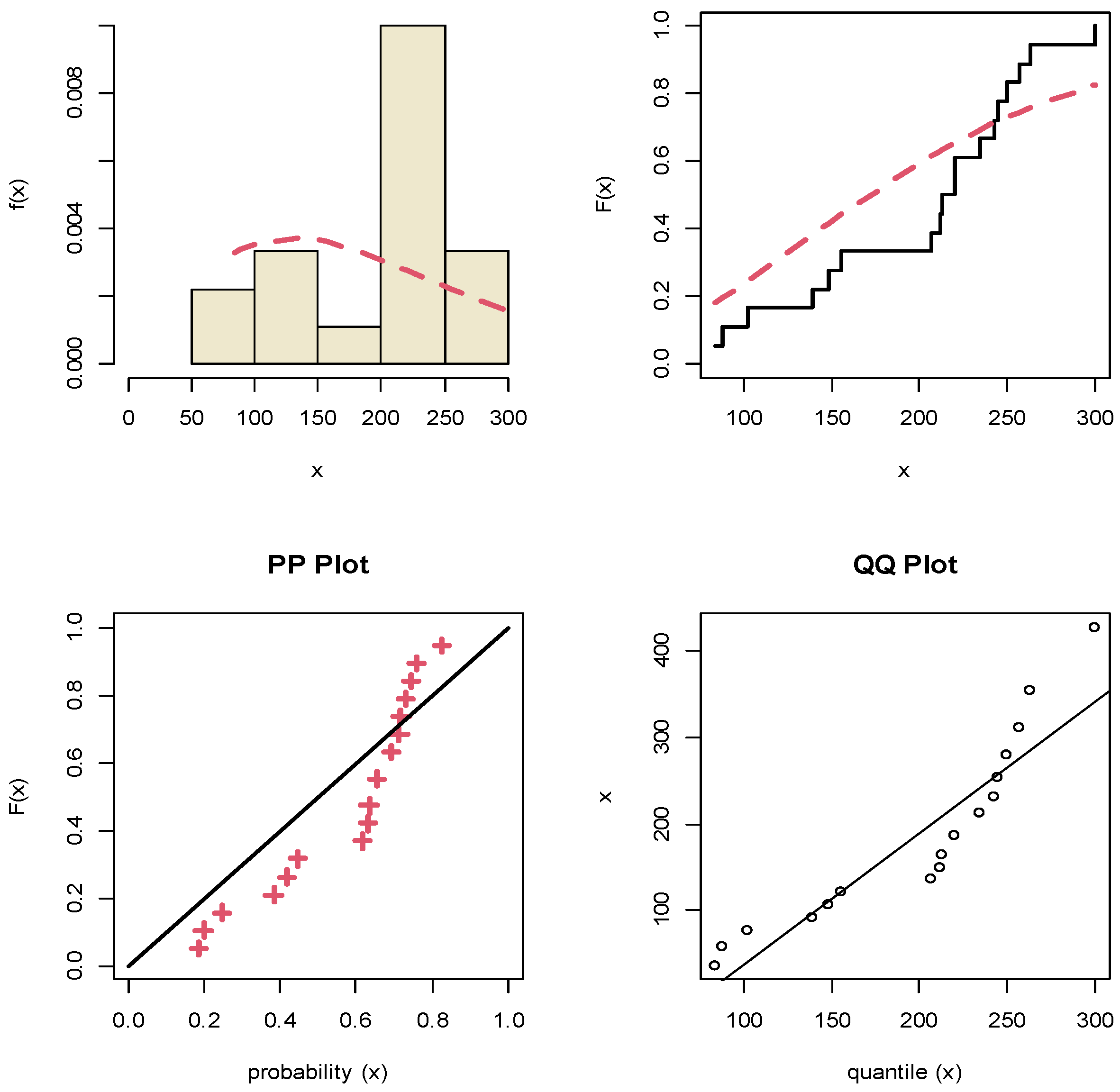
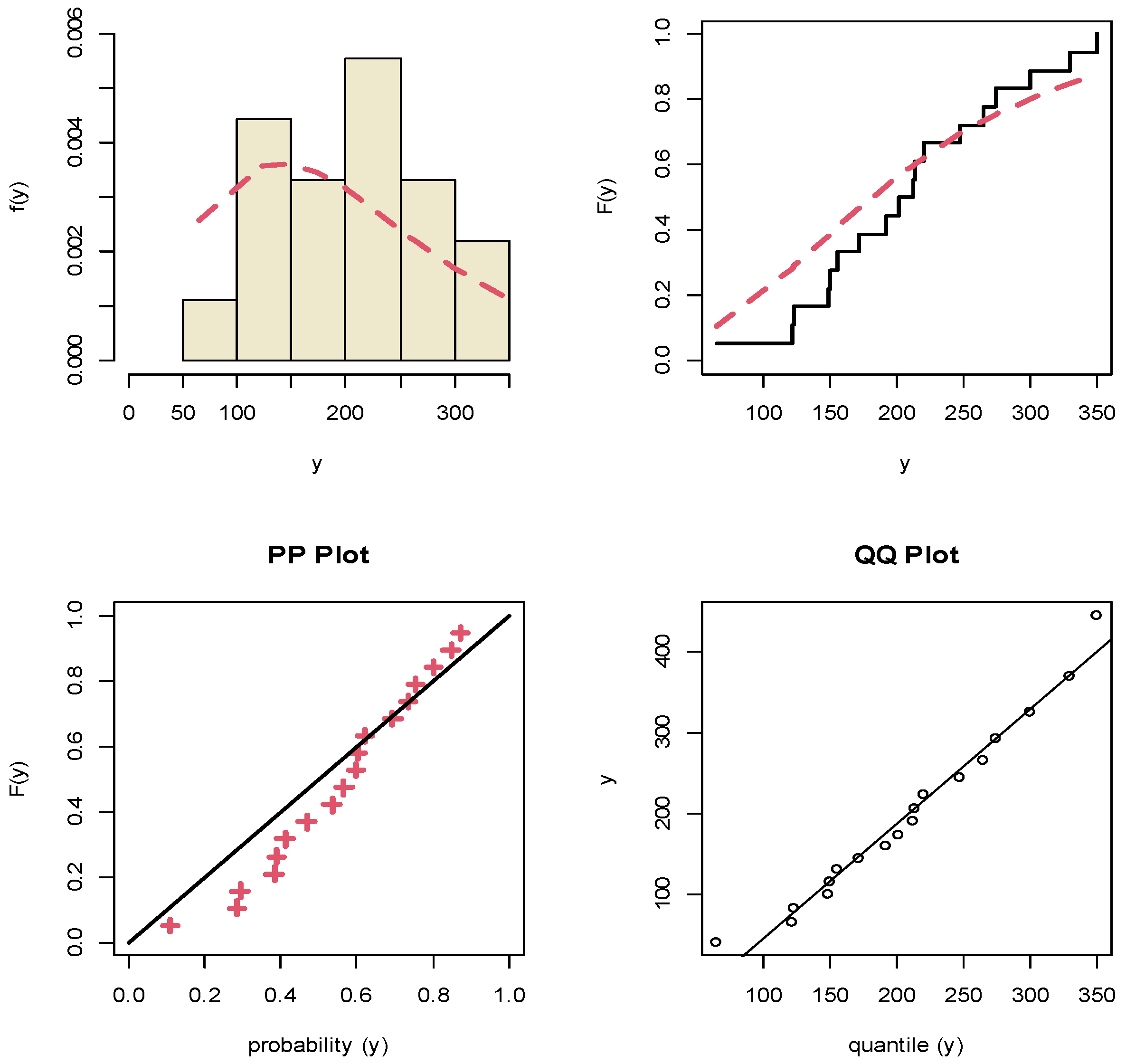
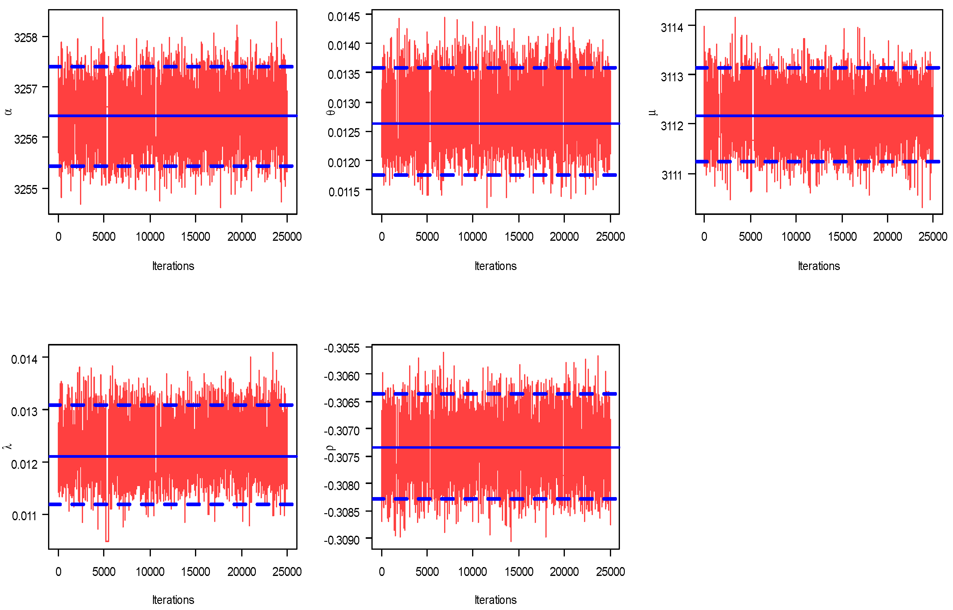
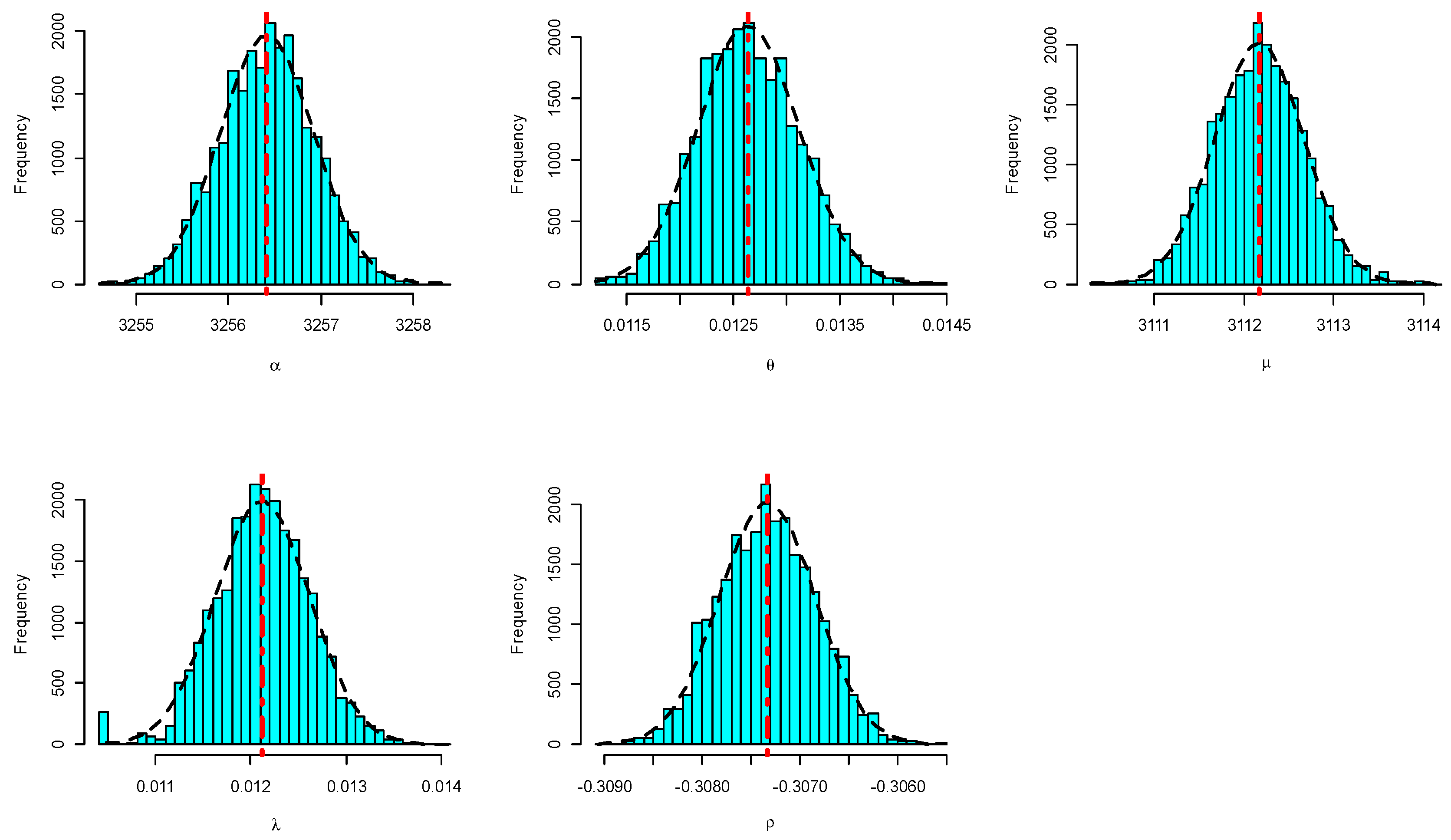
8. Motor Data Analysis

To demonstrate the practical utility of the proposed methodologies in an engineering phenomenon, one real data set reported by Ref. [47] is analyzed. This data represents the failure times (in days) of a parallel system constituted by two identical motors, namely, (X) and (Y), see Table 7. We first check the suitability of the APE model to the complete motor data sets. For this purpose, for each X and Y data point, the Kolmogorov–Smirnov (KS) statistics and its p -value, as well as the MLEs with their standard errors (SEs), are obtained and also provided in Table 7.
It shows that the APE distribution fits the motor data sets quite well. Moreover, some graphical methods for goodness of fit for the motor data sets are developed. Plots of fitted density, empirical cumulative distribution, probability-probability (PP) and quantile-quantile (QQ) for X and Y data sets are displayed in Figure 3 and Figure 4, respectively. It is clear that the two variables X and Y are fitted for the marginal APE distribution.
Using the complete X and Y data sets, the MLEs and 95% ACIs of α , θ , μ , λ and ρ are calculated. Furthermore, since no prior information is available about the MBAPE parameters, the Bayesian (point/credible) estimates of α , θ , μ , λ and ρ are developed using the non-informative priors. Taking the maximum likelihood estimates of the same unknown quantities as initial values, the MCMC sampler is replicated 30,000 times and then the first 5,000 iterations removed as a burn-in. The point (with their SEs) estimates and interval (with their lengths) estimates of the unknown parameters based on X and Y data sets are computed and listed in Table 8 and Table 9, respectively. This indicates that the estimates of the unknown parameters obtained by maximum likelihood and Bayesian methods are very similar. Moreover, trace plots (in Figure 5) for MCMC draws of the posterior generated samples of α , θ , μ , λ and ρ showed that the MCMC simulated variates converge very well. It represents the sample mean and two bounds of 95% BCIs with solid (—) and dashed (- - -) lines, respectively. Moreover, the MCMC frequency estimates of α , θ , μ , λ and ρ using the Gaussian kernel are represented in Figure 6. It represents the sample mean with a vertical dash-dotted (:) line. It is evident that the generated posteriors of all unknown parameters are quite symmetrical. To sum up, the numerical findings of the suggested estimation methods based on motor data provide a good demonstration of the proposed model.

9. Conclusions

In this paper, we propose and study a new class of bivariate alpha power distributions via finite mixtures involving APE distributions as marginals, and also consider the copula-based construction of bivariate alpha power distributions. The developed class of distribution is made up of two different types of mixture, namely, type I, which starts with two independent APE distributions, and type II, which starts with a bivariate Gaussian copula. The model parameters are estimated using both frequentist (for example, method of moments and the method of maximum likelihood) and under the Bayesian (using independent gamma priors) paradigm. This distribution can be employed in practice for non-negative and positively correlated random variables because the joint distribution function and joint density function are in closed forms; in addition, it can be applied to model censored data as well. Under the Bayesian paradigm, we adopted the EM approach, which works quite well and may be efficiently employed to compute the MLEs, because the MLEs of the unknown parameters cannot be computed in closed form. To compare the behavior/efficiency of the proposed methods and to see the applicability of the different estimators, a small simulation study is considered, and one real data set is investigated to examine the applicability of the proposed model. From the simulation study, it appears that the point and interval estimates of all unknown parameters using the MCMC algorithm are performing better. Therefore, the Bayes M-H method used to estimate the unknown MBAPE parameters is recommended. However, whether this is a general trend or not is subject to a separate study with a wide range of possible values of the model parameters.

Author Contributions

Formal analysis, A.E.; Funding acquisition, R.A.; Investigation, H.R.; Methodology, M.N. and I.G.; Project administration, R.A.; Resources, R.A.; Software, A.E.; Supervision, M.N. and H.R.; Writing—original draft, I.G. and A.E.; Writing—review & editing, H.R. All authors have read and agreed to the published version of the manuscript.

Funding

This research was funded by Princess Nourah bint Abdulrahman University Researchers Supporting Project number (PNURSP2022R50), Princess Nourah bint Abdulrahman University, Riyadh, Saudi Arabia.

Institutional Review Board Statement

Not applicable.

Informed Consent Statement

Not applicable.

Data Availability Statement

The data used to support the findings of this study are included within the article.

Acknowledgments

Princess Nourah bint Abdulrahman University Researchers Supporting Project number (PNURSP2022R50), Princess Nourah bint Abdulrahman University, Riyadh, Saudi Arabia).

Conflicts of Interest

The authors declare no conflict of interest.

Appendix A

Let us have a look at the BMAPE (type-I) distribution’s shape. From the joint density in (5), it is clear that there may be more than one critical point for the BMAPE (type-I) distribution. A numerical examination must be adopted for varying model parameter choices to obtain an idea of the critical points for this distribution
h 1 x , y x = a 1 α 1 1 μ 1 1 θ 2 log α 1 e 2 θ x α 1 e θ x 1 e θ x + θ e θ x α 1 1 e θ x λ log μ 1 e λ y μ 1 1 e λ y + b 1 α 1 1 μ 2 1 θ 2 log α 1 e 2 θ x α 1 e θ x 1 e θ x + θ e θ x α 1 1 e θ x λ log μ 2 e λ y μ 2 1 e λ y + c 1 α 2 1 μ 1 1 θ 2 log α 2 e 2 θ x α 2 e θ x 1 e θ x + θ e θ x α 2 1 e θ x λ log μ 1 e λ y μ 1 1 e λ y + d 1 α 2 1 μ 2 1 θ 2 log α 2 e 2 θ x α 2 e θ x 1 e θ x + θ e θ x α 2 1 e θ x λ log μ 2 e λ y μ 2 1 e λ y = 0 ,  
Also,
h 1 x , y y = a 1 α 1 1 μ 1 1 θ log α 1 e θ x α 1 1 e θ x + θ e θ x α 1 1 e θ x λ 2 log μ 1 e 2 λ y 1 e λ y μ 1 e λ y + λ e λ y μ 1 1 e λ y + b 1 α 1 1 μ 2 1 θ log α 1 e θ x α 1 1 e θ x λ 2 log μ 2 e 2 λ y 1 e λ y μ 2 e λ y + λ e λ y μ 2 1 e λ y + c 1 α 2 1 μ 1 1 θ log α 2 e θ x α 2 1 e θ x λ 2 log μ 1 e 2 λ y 1 e λ y μ 1 e λ y + λ e λ y μ 1 1 e λ y + d 1 α 2 1 μ 2 1 θ log α 2 e θ x α 2 1 e θ x λ 2 log μ 2 e 2 λ y 1 e λ y μ 2 1 e λ y + λ e λ y μ 2 1 e λ y = 0 .
From (A1) and (A2), it is evident that there will be more than one point for the BMAPE (type-I) distribution.

References

  1. Mahdavi, A.; Kundu, D. A new method for generating distributions with an application to exponential distribution. Commun. Stat.-Theory Methods 2017, 46, 6543–6557. [Google Scholar] [CrossRef]
  2. McLachlan, G.J.; Krishnan, T. The EM Algorithm and Extensions; John Wiley & Sons: New York, NY, USA, 1997. [Google Scholar]
  3. Mead, M.E.; Cordeiro, G.M.; Afify, A.Z.; Al Mofleh, H. The alpha power transformation family: Properties and applications. Pak. J. Stat. Oper. Res. 2019, 15, 525–545. [Google Scholar] [CrossRef]
  4. Newcomb, S. A generalized theory of the combination of observations so as to obtain the best result. Am. J. Math. 1886, 8, 343–366. [Google Scholar] [CrossRef]
  5. Pearson, K. Contributions to the Mathematical Theory of Evolution. Philos. Trans. A 1894, 185, 71–110. [Google Scholar]
  6. Titterington, D.M.; Smith, A.F.M.; Makov, U.E. Statistical Analysis of Finite Mixture Distributions; Wiley: New York, NY, USA, 1985. [Google Scholar]
  7. Everitt, B.S.; Hand, D.J. Finite Mixture Distributions; John Wiley & Sons, Ltd.: The Netherlands, 1981. [Google Scholar]
  8. McLachlan, G.J.; Basford, K.E. Mixture Models Inferences and Applications to Clustering; Marcel Dekker: New York, NY, USA, 1988. [Google Scholar]
  9. Al-Hussaini, E.K.; Sultan, K.S. Reliability and hazard based on finite mixture Models. In Handbook of Statistics; Balakrishnan, N., Rao, C.R., Eds.; Handbook of Statistics: Amsterdam, The Netherlands, 2001; Volume 20, pp. 139–183. [Google Scholar]
  10. AL-Moisheer, A.S.; Alotaibi, R.M.; Alomani, G.A.; Rezk, H.R. Bivariate Mixture of Inverse Weibull Distribution: Properties and Estimation. Math. Probl. Eng. 2020, 2020, 5234601. [Google Scholar] [CrossRef]
  11. Nassar, M.; Alzaatreh, A.; Mead, M.; Abo-Kasem, O. Alpha power Weibull distribution: Properties and applications. Commun. Stat.-Theory Methods 2017, 46, 10236–10252. [Google Scholar] [CrossRef]
  12. Dey, A.; Alzaatreh, A.; Zhang, C.; Kumar, D. A new extension of generalized exponential distribution with application to ozone data. Ozone Sci. Eng. 2017, 39, 273–285. [Google Scholar] [CrossRef]
  13. Nadarajah, S.; Okorie, I.E. On the moments of the alpha power transformed generalized exponential distribution. Ozone Sci. Eng. 2018, 40, 330–335. [Google Scholar] [CrossRef]
  14. Nassar, M.; Afify, A.Z.; Dey, S.; Kumar, D. A new extension of Weibull distribution: Properties and different methods of estimation. J. Comput. Appl. Math. 2018, 336, 439–457. [Google Scholar] [CrossRef]
  15. Nassar, M.; Kumar, D.; Dey, S.; Cordeiro, G.M.; Afify, A.Z. The Marshall–Olkin alpha power family of distributions with applications. J. Comput. Appl. Math. 2019, 351, 41–53. [Google Scholar] [CrossRef]
  16. Nassar, M.; Afify, A.; Shakhatreh, M. Estimation Methods of Alpha Power Exponential Distribution with Applications to Engineering and Medical Data. Pak. J. Stat. Oper. Res. 2020, 16, 149–166. [Google Scholar] [CrossRef]
  17. Jaheen, Z. On record statistics from a mixture of two exponential distributions. J. Stat. Comput. Simul. 2005, 75, 1–11. [Google Scholar] [CrossRef]
  18. Al-Hussaini, E.K.; Hussein, M. Estimation under a Finite Mixture of Exponentiated Exponential Components Model and Balanced Square Error Loss. Open J. Stat. 2012, 2, 28–38. [Google Scholar] [CrossRef]
  19. Tahir, M.; Aslam, M.; Hussain, Z.; Khan, A. On finite 3-component mixture of exponential distributions: Properties and estimation. Cogent Math. 2016, 3, 1275414. [Google Scholar] [CrossRef]
  20. Diawara, N.; Carpenter, M. Mixture of bivariate exponential distributions. Commun. Stat.-Theory Methods 2010, 39, 2711–2720. [Google Scholar] [CrossRef]
  21. Rafiei, M.; Iranmanesh, A.; Nagar, D. A bivariate gamma distribution whose marginals are finite mixtures of gamma distributions. Stat. Optim. Inf. Comput. 2020, 8, 950–971. [Google Scholar] [CrossRef]
  22. Mardia, K.V. Measures of multivariate skewness and kurtosis with applications. Biometrika 1970, 57, 519–530. [Google Scholar] [CrossRef]
  23. Kotz, S.; Balakrishnan, N.; Johnson, N. Continuous Multivariate Distributions: Models and Applications, 2nd ed.; Wiley: New York, NY, USA, 2000; Volume 1. [Google Scholar]
  24. Balakrishnan, N.; Lai, C. Cotinuous Bivariate Distributions, 2nd ed.; Springer: New York, NY, USA, 2009. [Google Scholar]
  25. Nelson, R.B. An Introduction to Copulas; Springer: New York, NY, USA, 2006. [Google Scholar]
  26. Dellaert, F. The Expectation Maximization Algorithm; CiteSeerX 10.1.1.9.9735. gives an easier explanation of EM algorithm as to lowerbound maximization 2002; Georgia Institute of Technology: Atlanta, GA, USA, 2002. [Google Scholar]
  27. Kundu, D. Bivariate sinh-normal distribution and a related model. Braz. J. Probab. Stat. 2015, 29, 590–607. [Google Scholar] [CrossRef]
  28. El-Morshedy, M.; Alhussain, Z.A.; Atta, D.; Almetwally, E.M.; Eliwa, M.S. Bivariate Burr X Generator of Distributions: Properties and Estimation Methods with Applications to Complete and Type-II Censored Samples. Mathematics 2020, 8, 264. [Google Scholar] [CrossRef]
  29. Alotaibi, R.; Rezk, H.; Ghosh, I.; Dey, S. Bivariate exponentiated half logistic distribution: Properties and application. Commun. Stat.-Theory Methods 2020, 50, 6099–6121. [Google Scholar] [CrossRef]
  30. Sklar, A. Fonctions de Répartition à n Dimensions et Leurs Marges; Publications de l’Institut Statistique de l’Université de Paris: Paris, France, 1959; Volume 8, pp. 229–231. [Google Scholar]
  31. Kosmidis, I.; Karlis, D. Model-based clustering using copulas with applications. Stat. Comput. 2016, 26, 1079–1099. [Google Scholar] [CrossRef]
  32. Joe, H.; Xu, J. The Estimation Method of Inference Functions for Margins for Multivariate Models; Technical Report No. 166; Department of Statistics, University of British Columbia: Vancouver, BC, Canada, 1996. [Google Scholar]
  33. Kojadinovic, I.; Yan, J. Comparison of three semiparametric methods for estimating dependence parameters in copula models. Insur. Math. Econ. 2010, 47, 52–63. [Google Scholar] [CrossRef]
  34. Fermanian, J.D. Goodness-of-fit tests for copulas. J. Multivar. Anal. 2005, 95, 119–152. [Google Scholar] [CrossRef]
  35. Dobric, J.; Schmid, F. A goodness of fit test for copulas based on Rosenblatt’s transformation. Comput. Stat. Data Anal. 2007, 51, 4633–4642. [Google Scholar] [CrossRef]
  36. Genest, C.; Remillard, B. Validity of the parametric bootstrap for goodness-of-fit testing in semiparametric models. Ann. L’institut Henri Poincare (B) Probab. Stat. 2008, 44, 1096–1127. [Google Scholar] [CrossRef]
  37. Genest, C.; Rémillard, B.; Beaudoin, D. Goodness-of-fit tests for copulas: A review and a power study. Insur. Math. Econ. 2009, 44, 199–213. [Google Scholar] [CrossRef]
  38. Kojadinovic, I.; Yan, J.; Holmes, M. Fast large-sample goodness-of-fit tests for copulas. Stat. Sin. 2011, 21, 841–871. [Google Scholar] [CrossRef]
  39. Meintanis, S.G. Test of fit for Marshall–Olkin distributions with applications. J. Stat. Plan. Inference 2007, 137, 3954–3963. [Google Scholar] [CrossRef]
  40. Metropolis, N.; Rosenbluth, A.W.; Rosenbluth, M.N.; Teller, A.H. Equation of state calculations by fast computing machines. J. Chem. Phys. 1953, 21, 1087–1091. [Google Scholar] [CrossRef]
  41. Hastings, W.K. Monte Carlo sampling methods using Markov chains and their applications. Biometrika 1970, 57, 97–109. [Google Scholar] [CrossRef]
  42. Plummer, M.; Best, N.; Cowles, K.; Vines, K. Convergence diagnosis and output analysis for MCMC. R News 2006, 6, 7–11. [Google Scholar]
  43. Henningsen, A.; Toomet, O. maxLik: A package for maximum likelihood estimation in R. Comput. Stat. 2011, 26, 443–458. [Google Scholar] [CrossRef]
  44. Gilks, W.R.; Best, N.G.; Tan, K.K.C. Adaptive Rejection Metropolis Sampling within Gibbs Sampling. Appl. Stat. 1995, 44, 455–472. [Google Scholar] [CrossRef]
  45. Martino, L.; Yang, H.; Luengo, D.; Kanniainen, J.; Corander, J. A Fast Universal Self-Tuned Sampler Within Gibbs Sampling. Digit. Signal Process. 2015, 47, 68–83. [Google Scholar] [CrossRef]
  46. Fitzgerald, W.J. Markov chain Monte Carlo methods with applications to signal processing. Signal Process. 2001, 81, 3–18. [Google Scholar] [CrossRef]
  47. Alotaibi, R.; Khalifa, M.; Almetwally, E.; Ghosh, I.; Rezk, H. Classical and Bayesian Inference of a Mixture of Bivariate Exponentiated Exponential Model. J. Math. 2021, 2021, 5200979. [Google Scholar] [CrossRef]
Figure 1. Joint density plot of the BMAPE (type-I) distribution for the selected parameter choices.
Axioms 11 00459 g001
Figure 2. Contour plot of the BMAPE (type-I) distribution for the selected parameter choices.
Axioms 11 00459 g002
Figure 3. The fitted density, empirical CDF, PP and QQ plots under X data.
Axioms 11 00459 g003
Figure 4. The fitted density, empirical CDF, PP and QQ plots under Y data.
Axioms 11 00459 g004
Figure 5. MCMC trace plots of α , θ , μ , λ and ρ under motor data set.
Axioms 11 00459 g005
Figure 6. MCMC frequency estimates plots of α , θ , μ , λ and ρ under motor data set.
Axioms 11 00459 g006
Table 1. Different parameter values under independent/dependent cases.
ParameterTrue ValuePrior 1Prior 2True ValuePrior 1Prior 2
w m w m w m w m
Set   III
α 0.40.822.050.81.624.05
θ 0.51.022.551.53.027.55
μ 0.20.421.050.42.022.05
λ 0.81.624.051.22.426.05
ρ 0.30.621.550.51.025.05
Set   IIIIV
α 1 0.10.220.550.30.621.55
α 2 0.30.621.550.51.022.55
θ 0.51.022.551.53.027.55
μ 1 0.10.220.550.20.421.05
μ 2 0.10.220.550.20.421.05
λ 0.81.624.051.22.425.05
Table 2. Simulated point and interval estimates of the BMAPE parameters for Sets I and II.
Set n Par.MLEMCMC.1MCMC.2ACIBCI.1BCI.2
MABRMSEMABRMSEMABRMSE
I50 α 0.6181.1060.1430.1990.0370.0643.0560.3480.092
θ 0.1710.2170.1080.1540.0390.0590.7270.3000.099
μ 0.4010.7640.1790.2050.1020.1772.0400.2960.250
λ 0.3140.4090.2620.3950.2030.3431.4020.6580.492
ρ 0.3040.3630.2610.3350.1660.2900.6360.5250.392
100 α 0.3510.5270.1270.1870.0360.0581.7710.3460.089
θ 0.1180.1550.0960.1250.0370.0560.5520.2500.093
μ 0.2460.3880.1530.1980.0970.1651.2260.2740.242
λ 0.2420.3750.2400.3500.2000.3011.1100.6480.474
ρ 0.3020.3170.2310.2910.1640.2790.5750.4050.390
150 α 0.2630.3770.1220.1810.0340.0551.3380.2860.087
θ 0.0970.1510.0790.1010.0360.0510.4580.2490.086
μ 0.1860.2770.1030.1630.0960.1410.9180.2660.236
λ 0.2020.3400.1980.2580.1520.2260.9750.4800.352
ρ 0.3010.3110.2250.2850.1620.2770.5550.3990.319
200 α 0.2240.3140.1160.1550.0320.0541.1210.2820.084
θ 0.0840.1090.0380.0610.0320.0450.3980.1130.076
μ 0.1770.2210.0990.1530.0950.1400.7510.2590.230
λ 0.1920.3350.1790.2260.1500.2200.8470.4640.347
ρ 0.3000.3060.2110.2800.1600.2670.5030.3920.276
II50 α 0.9071.5830.2720.4430.1070.1834.9880.6760.265
θ 0.3730.4820.2760.4370.2230.3961.8150.7260.550
μ 0.5911.0460.3680.6280.3600.6213.1611.0620.867
λ 0.3950.5620.3110.4610.2660.4531.7940.8830.644
ρ 0.5030.5510.4700.5050.2360.4121.0570.5730.551
100 α 0.5460.8190.2680.4040.1050.1772.8660.6400.258
θ 0.2930.4520.2620.3870.2210.3921.2950.6980.544
μ 0.4230.6930.3550.6210.3540.5681.8101.0330.857
λ 0.3460.5090.2880.4510.2550.3721.3280.7990.630
ρ 0.5020.5250.3480.4760.2330.4000.8360.5710.392
150 α 0.4270.6100.2540.3980.1010.1732.1790.6090.248
θ 0.2680.4370.2260.3780.2160.3381.0690.6950.542
μ 0.4070.6720.3510.6180.2700.3921.3261.0300.851
λ 0.3150.4870.2580.4440.2340.2991.1030.7640.626
ρ 0.5010.5120.3390.4010.2300.3990.7890.5580.319
200 α 0.3650.5140.2180.3200.0980.1691.8270.5210.243
θ 0.2440.3920.2230.2770.1840.2330.9140.6140.539
μ 0.4000.6480.3260.5580.2250.3131.1240.8620.832
λ 0.3070.4530.2550.4420.2000.2570.9590.6240.619
ρ 0.5000.5090.3170.3990.2290.3810.7640.5520.277
Table 3. Simulated point and interval estimates of the BMAPE parameters using Set III when ρ 11 , ρ 12 , ρ 21 , ρ 22 = 0.2 , 0.15 , 0.05 , 0.1 .
n Par.MLEMCMC.1MCMC.2ACIBCI.P1BCI.P2
MABRMSEMABRMSEMABRMSE
50 α 1 0.0850.1130.0580.0610.0390.0440.6060.0850.074
α 2 0.2740.2950.0730.0810.0290.0310.6300.1430.077
θ 0.2730.2630.2280.0620.2080.0600.7790.0990.056
μ 1 0.0870.1230.0610.0630.0490.0530.4550.1330.055
μ 2 0.0990.1060.0870.1040.0450.0460.5280.1160.068
λ 0.3230.3590.0530.0630.0180.0191.8140.1290.041
ρ 11 0.3880.4110.2240.2340.1720.1780.5140.2470.195
ρ 12 0.4280.4470.1840.1940.1410.1440.5540.2280.162
ρ 21 0.4090.4420.1660.1760.1120.1150.6020.1800.156
ρ 22 0.4270.4510.1660.1800.1630.1710.6780.2540.154
100 α 1 0.0840.1010.0480.0510.0230.0250.2060.0830.070
α 2 0.2680.2870.0410.0530.0240.0240.5490.1050.067
θ 0.2390.2600.2200.0350.1760.0150.5570.0790.038
μ 1 0.0860.1080.0500.0580.0450.0510.3880.1040.053
μ 2 0.0850.1010.0350.0440.0250.0300.3210.1010.061
λ 0.3220.3580.0470.0580.0150.0161.0450.1170.040
ρ 11 0.3640.3910.1730.1810.1450.1580.3940.1920.139
ρ 12 0.4200.4450.1570.1720.1090.1190.3810.2010.117
ρ 21 0.4070.4390.1270.1360.0500.0590.4510.1610.097
ρ 22 0.4220.4500.1130.1190.0530.0610.4490.1300.128
150 α 1 0.0830.0960.0250.0280.0220.0220.2010.0690.066
α 2 0.2670.2730.0400.0450.0180.0220.5390.0920.040
θ 0.2350.2570.2120.0340.1700.0130.5190.0760.037
μ 1 0.0860.1040.0430.0460.0120.0150.3210.0990.052
μ 2 0.0830.0970.0260.0310.0190.0240.2440.0780.037
λ 0.3190.3560.0380.0410.0140.0150.8210.0690.037
ρ 11 0.3650.3880.0870.0890.0610.0620.3480.0740.040
ρ 12 0.4190.4350.1290.1300.0680.0780.3500.1390.060
ρ 21 0.4010.4290.0590.0670.0410.0440.3640.0940.076
ρ 22 0.4090.4400.0750.0800.0170.0180.4100.1210.026
200 α 1 0.0790.0860.0210.0250.0190.0210.1630.0500.016
α 2 0.2580.2690.0350.0400.0140.0180.3470.0800.019
θ 0.2320.2470.1710.0240.1670.0100.4130.0700.013
μ 1 0.0840.0990.0390.0450.0050.0060.2650.0680.015
μ 2 0.0810.0910.0220.0230.0110.0130.2010.0490.020
λ 0.2990.3430.0220.0280.0090.0110.8010.0570.013
ρ 11 0.3580.3820.0300.0310.0180.0230.2980.0630.011
ρ 12 0.4150.4340.0340.0380.0100.0110.3040.0540.019
ρ 21 0.3920.4250.0500.0500.0400.0420.3610.0570.008
ρ 22 0.4080.4380.0430.0590.0140.0150.3750.0950.008
Table 4. Simulated point and interval estimates of the BMAPE parameters using Set III when ρ 11 , ρ 12 , ρ 21 , ρ 22 = 0.5 , 0.4 , 0.2 , 0.3 .
n Par.MLEMCMC.1MCMC.2ACIBCI.P1BCI.P2
MABRMSEMABRMSEMABRMSE
50 α 1 0.0950.1440.0650.0670.0450.0560.8070.1290.083
α 2 0.2530.3940.0700.0730.0330.0351.5650.1430.090
θ 0.2120.1820.1740.0870.1430.0221.2320.1540.042
μ 1 0.0910.1240.0530.0540.0410.0490.9710.1220.058
μ 2 0.0840.1250.0560.0640.0320.0370.7860.0940.068
λ 0.2320.2770.1120.1150.0460.0482.0560.1260.067
ρ 11 0.1530.1890.0980.1070.0530.0560.5160.1820.097
ρ 12 0.2300.2520.1980.2140.0630.0720.5340.2600.124
ρ 21 0.3350.3480.1120.1200.0320.0360.6200.1380.093
ρ 22 0.2680.2860.2170.2320.0350.0400.6450.2350.122
100 α 1 0.0780.1330.0600.0630.0430.0540.6960.1150.077
α 2 0.2200.2380.0590.0660.0300.0320.7870.1200.079
θ 0.2100.1770.1700.0490.1370.0111.0300.1170.039
μ 1 0.0770.0910.0470.0520.0340.0380.7580.1010.054
μ 2 0.0790.1010.0390.0420.0190.0230.6950.0920.061
λ 0.2160.2550.0680.0720.0270.0321.7520.0910.052
ρ 11 0.1420.1710.0820.1020.0420.0470.4820.1460.066
ρ 12 0.2270.2440.1020.1110.0380.0400.5240.1700.070
ρ 21 0.3330.3460.0990.1050.0310.0330.5760.1330.073
ρ 22 0.2660.2830.1060.1190.0290.0340.6020.1820.087
150 α 1 0.0670.0870.0570.0620.0360.0410.5620.1130.068
α 2 0.2190.2360.0370.0470.0270.0300.7160.1110.060
θ 0.2070.1650.1520.0460.1310.0100.8310.0800.024
μ 1 0.0750.0890.0450.0500.0130.0140.7080.1000.034
μ 2 0.0780.0980.0330.0380.0120.0140.5490.0790.054
λ 0.2050.2490.0590.0700.0200.0211.6920.0900.040
ρ 11 0.1350.1670.0450.0530.0360.0440.4520.1000.065
ρ 12 0.2150.2420.0860.0940.0170.0220.4180.1540.068
ρ 21 0.3320.3450.0600.0690.0230.0240.5300.1240.039
ρ 22 0.2570.2810.1000.1110.0210.0320.5270.1780.083
200 α 1 0.0660.0740.0320.0390.0310.0370.4940.0850.052
α 2 0.2170.2330.0250.0310.0230.0280.5470.0900.043
θ 0.1800.1580.1470.0250.1300.0080.8040.0680.022
μ 1 0.0680.0810.0350.0410.0090.0120.6910.0920.032
μ 2 0.0670.0760.0290.0320.0110.0110.5440.0760.052
λ 0.2020.2430.0460.0480.0190.0201.5100.0520.038
ρ 11 0.1330.1630.0420.0470.0220.0270.3900.0840.062
ρ 12 0.2140.2330.0650.0760.0150.0200.3880.1170.043
ρ 21 0.3300.3440.0360.0430.0200.0220.5280.0990.035
ρ 22 0.2490.2600.0450.0560.0190.0300.5100.1500.060
Table 5. Simulated point and interval estimates of the BMAPE parameters using Set IV when ρ 11 , ρ 12 , ρ 21 , ρ 22 = 0.2 , 0.15 , 0.05 , 0.1 .
𝒏Par.MLEMCMC.1MCMC.2ACIBCI.P1BCI.P2
MABRMSEMABRMSEMABRMSE
50 α 1 0.2350.3070.0650.0700.0380.0442.6100.1090.084
α 2 0.3490.4320.0700.0780.0560.0202.9260.1410.079
θ 0.9740.4560.3830.0620.0700.0273.1670.1040.060
μ 1 0.1600.2130.0760.0780.0610.0681.7580.1910.073
μ 2 0.1790.2500.0970.1030.0490.0532.3600.1130.110
λ 0.3380.3940.0750.0830.0230.0292.8430.1510.048
ρ 11 0.4270.4480.2290.2400.1710.1800.5070.2530.199
ρ 12 0.4750.4920.1860.1970.1470.1500.5410.2280.163
ρ 21 0.5240.5380.1670.1770.1120.1150.6960.1820.159
ρ 22 0.4950.5080.1640.1810.1620.1660.6770.2520.147
100 α 1 0.1980.2290.0490.0530.0320.0391.3880.0990.081
α 2 0.3380.3790.0420.0550.0290.0292.3240.1020.078
θ 0.9440.4450.3480.0570.0210.0192.4780.1000.044
μ 1 0.1440.1750.0620.0650.0570.0631.4100.1040.066
μ 2 0.1520.1960.0440.0490.0290.0341.2610.0990.065
λ 0.3050.3730.0650.0790.0140.0171.9820.1220.036
ρ 11 0.4170.4270.1800.1850.1460.1600.4710.1920.147
ρ 12 0.4730.4830.1540.1690.1110.1220.4350.2180.140
ρ 21 0.5080.5200.1280.1380.0460.0580.5760.1630.100
ρ 22 0.4810.4930.1130.1200.0540.0620.5350.1310.130
150 α 1 0.1830.2440.0390.0450.0220.0271.2800.0760.069
α 2 0.3200.3530.0400.0450.0270.0311.8160.0870.044
θ 0.8730.4280.2660.0410.0070.0132.1990.0820.038
μ 1 0.1380.1730.0390.0460.0130.0151.0040.1000.053
μ 2 0.1470.1860.0370.0480.0170.0201.1050.0610.056
λ 0.3010.3620.0470.0570.0130.0151.8600.1120.034
ρ 11 0.4070.4200.0900.0920.0640.0650.4410.0780.067
ρ 12 0.4670.4810.1410.1430.0700.0800.4270.1190.098
ρ 21 0.5070.5170.0570.0650.0400.0420.5430.0930.089
ρ 22 0.4790.4920.0750.0810.0460.0520.5250.1250.096
200 α 1 0.1820.2360.0280.0280.0190.0211.0160.0420.019
α 2 0.3180.3520.0310.0360.0160.0561.7570.0840.034
θ 0.3820.3990.0380.0260.0030.0111.8660.0770.025
μ 1 0.1280.1500.0280.0330.0100.0110.8570.0610.026
μ 2 0.1320.1530.0130.0180.0120.0130.9200.0500.025
λ 0.2850.3540.0280.0300.0120.0141.6250.0700.032
ρ 11 0.4020.4120.0610.0630.0190.0260.4390.0440.038
ρ 12 0.4640.4740.0360.0400.0050.0060.3860.0550.021
ρ 21 0.5060.5160.0490.0490.0380.0410.5110.0590.010
ρ 22 0.4660.4760.0710.0730.0220.0250.5100.0560.051
Table 6. Simulated point and interval estimates of the BMAPE parameters using Set IV when ρ 11 , ρ 12 , ρ 21 , ρ 22 = 0.5 , 0.4 , 0.2 , 0.3 .
𝒏Par.MLEMCMC.1MCMC.2ACIBCI.P1BCI.P2
MABRMSEMABRMSEMABRMSE
50 α 1 0.2500.4120.0720.0770.0560.0712.5450.1570.087
α 2 0.3740.5530.0850.0930.0780.0813.7380.1430.077
θ 0.9960.3520.2770.0590.0850.0512.7930.1040.060
μ 1 0.2070.3120.0780.0830.0740.0802.3690.2050.071
μ 2 0.2190.3470.0930.0990.0770.0902.6210.1390.108
λ 0.2810.3540.0600.0720.0220.0272.7860.1320.068
ρ 11 0.1750.2110.1600.1680.0600.0720.6480.2360.113
ρ 12 0.2180.2470.0990.1010.0490.0610.5410.1370.120
ρ 21 0.3450.3630.1690.1760.0810.0930.7580.1910.130
ρ 22 0.2610.2800.2340.2470.0320.0430.6790.2410.107
100 α 1 0.2470.3470.0600.0640.0400.0451.8360.1040.085
α 2 0.3260.4070.0500.0560.0340.0372.9580.1170.074
θ 0.9850.3270.2600.0500.0500.0212.1950.0980.055
μ 1 0.2010.2840.0650.0760.0430.0501.8180.1540.063
μ 2 0.2110.3300.0620.0690.0310.0372.2470.1100.066
λ 0.2460.3140.0500.0600.0180.0252.1470.1250.043
ρ 11 0.1590.1900.1440.1590.0310.0410.4600.1630.096
ρ 12 0.2140.2300.0610.0700.0200.0240.4590.1300.064
ρ 21 0.3440.3610.1370.1480.0380.0460.5270.1800.125
ρ 22 0.2580.2760.1360.1460.0310.0370.5750.2080.097
150 α 1 0.2180.3290.0460.0470.0250.0291.7010.1010.083
α 2 0.3110.4140.0360.0450.0190.0232.6230.0890.070
θ 0.9740.3040.2410.0410.0130.0121.8720.0940.039
μ 1 0.1720.2270.0630.0670.0130.0161.1670.0980.057
μ 2 0.2030.2950.0400.0450.0160.0191.6280.0940.058
λ 0.2360.3010.0370.0410.0130.0141.6000.0960.041
ρ 11 0.1570.1870.0860.0890.0290.0330.4300.1000.082
ρ 12 0.2090.2250.0340.0420.0120.0160.4230.0660.054
ρ 21 0.3370.3510.1100.1170.0240.0280.4870.1400.058
ρ 22 0.2540.2680.1030.1160.0300.0320.4900.1790.081
200 α 1 0.1590.2010.0380.0450.0100.0121.2330.0480.039
α 2 0.2680.3140.0310.0370.0140.0192.0810.0840.042
θ 0.9220.2710.1840.0290.0100.0101.5700.0800.036
μ 1 0.1480.2020.0290.0340.0110.0121.0890.0650.050
μ 2 0.1560.2090.0220.0250.0110.0141.2690.0490.041
λ 0.2260.2810.0290.0330.0110.0121.5710.0710.037
ρ 11 0.1490.1750.0480.0550.0230.0290.3630.0920.052
ρ 12 0.2000.2190.0290.0350.0110.0150.3710.0610.044
ρ 21 0.3330.3430.0840.0940.0180.0200.4290.1320.034
ρ 22 0.2520.2650.0740.0820.0180.0240.4490.1760.042
Table 7. Failure times of two motors.
MotorFailure TimesMLE(SE)KS
α θ Statistic p -Value
X84, 88, 102, 139, 148, 156, 207, 212, 213, 220, 220, 235, 243, 245, 250, 257, 263, 30039.044 (29.274)0.0099 (0.0016)0.28290.112
Y65, 121, 123, 148, 150, 156, 172, 192, 202, 212, 214, 220, 248, 265, 275, 300, 330, 35047.906 (38.493)0.0096 (0.0015)0.22890.260
Table 8. The point estimates of α , θ , μ , λ and ρ under motor data.
Method α θ μ λ ρ
MLE
(SE)
3256.43
(0.0056)
0.01312
(0.0014)
3112.19 (8.3910)0.01262 (0.0014)−0.30736 (0.2181)
Bayes
(SE)
3256.41
(0.0032)
0.01263
(0.0001)
3112.17 (0.0031)0.01212
(0.0001)
−0.30733 (0.0001)
Table 9. The 95% interval estimates of α , θ , μ , λ and ρ under motor data.
Method α θ μ λ ρ
ACI
(length)
(3256.4,3256.4)
(0.0218)
(0.0103,0.0160)
(0.0057)
(3095.8,3128.6)
(32.894)
(0.0099,0.0154)
(0.0055)
(−0.7347,0.1200)
(0.8547)
BCI
(length)
(3255.4,3257.4)
(1.9753)
(0.0118,0.0136)
(0.0018)
(3111.2,3113.2)
(1.9131)
(0.0112,0.0131)
(0.0019)
(−0.3083,−0.3064)
(0.0019)
Publisher’s Note: MDPI stays neutral with regard to jurisdictional claims in published maps and institutional affiliations.

