Statistical Inference for Odds Ratio of Two Proportions in Bilateral Correlated Data

Abstract

Bilateral correlated data frequently arise in medical clinical studies such as otolaryngology and ophthalmology. Based on an equal correlation coefficient model, this paper mainly aimed to investigate the statistical inference for the odds ratio of two proportions in bilateral correlated data, including not only three test procedures but also four confidence interval (CI) constructions. Through iterative algorithms, all unknown parameters are estimated in order to construct the likelihood ratio, score and Wald-type tests. Furthermore, the profile likelihood CI, score CI, and Wald-type CI are obtained by the bisection root-finding algorithm. We provided another Wald-type CI based on an asymptotic normality property. The performance of the proposed tests were investigated with regard to empirical type I error rate and power, and CI methods were compared in terms of mean coverage probability and mean interval width. Numerical simulations show that the score test is more robust, and has higher power than other tests. The score CI also has a shorter interval width, and its coverage probability is closer to 0.95. A real example is used to illustrate the proposed methods.

1. Introduction

Binary data are often encountered when an investigator takes measurements from the paired organs of a patient. Observations may be related because they come from the same patient, such as both eyes, hands, arms, legs, or sides of the face [1,2,3,4]. For example, Mandel et al. [5] conducted a double-blind randomized clinical trial to compare cefaclor and amoxicillin for the treatment of otitis media with effusion in children with bilateral tympanocentesis. Sainani [6] reviewed some examples of correlated data and demonstrated that errors arise when correlations are ignored. Therefore, the misleading statistical inference may be obtained from ignoring the correlation between the responses of paired organs [7,8].

For the correlated binary outcomes, we briefly reviewed the developments of three main statistical models: Ronser’s model, Dallal’s model, and Donner’s model. An interclass correlation model was proposed by Ronser [9] based on the assumption that the probability of a response at one side given a response at the other side is proportional to the prevalence rate of the corresponding group. Ma et al. [10] analyzed the equality of the response rates for multiple groups under Ronser’s model. Tang et al. [11,12] proposed the test procedures and asymptotic confidence intervals (CIs) about risk differences based on Ronser’s model. Dallal [13] pointed out that Ronser’s model will give a poor fit if the characteristic is almost certain to occur bilaterally with widely varying group-specific prevalence and then considered that the probability of a response at one side given a response at the other side to be constant. Under Dallal’s model, Sun et al. [14] derived risk difference tests for stratified binary data. However, Dallal’s model had its own limitation. Furthermore, Donner [15] established an alternative model when the correlation coefficient between two paired organs is a fixed constant $\rho$. Liu et al. [16] derived several statistics from testing the equality of correlation coefficients for paired binary data. Pei et al. [17] constructed CI methods for risk differences under Donner’s model. Under these models, the risk difference, relative risk ratio, and odds ratio are the three most used methods to compare disease risk among different groups. In the first two forms, various approaches were used to describe and quantify the statistical inference in a given population. For more details about this topic, we refer the reader to [18,19,20,21,22,23]. However, the research into the odds ratio is still in its infancy and has had fewer achievements for the bilateral correlated data.

It is noteworthy that the odds ratio is a preferred measure of association in prospective, retrospective, or cross-sectional sampling designs. However, most of the aforementioned results usually focus on the test or CI problems of risk difference and relative risk ratio. In this paper, we focused on the study of statistical inference for the odds ratio of two proportions in bilateral correlated data. Under Donner’s model, the novelty and contribution embody several aspects: (i) three statistics are proposed to test whether the odds ratio $\delta$ of response rates equals a specific value ${\delta }_0$. The performance of these statistics is investigated in terms of type I error rate and power. (ii) We propose the use of CI methods for any specific value ${\delta }_0$. These intervals have some advantages; they contain the true value with a given probability. In addition, these can answer the testing problem and give a range of values for ${\delta }_0$. The remainder of the paper is organized as follows. In Section 2, we briefly review some notations, data structure, and Donner’s model. The unconstrained and constrained MLEs are obtained in Section 3. Three different test procedures are proposed in Section 4, and four asymptotic CI methods are provided in Section 5. In Section 6, the simulation studies were conducted to investigate the performance of three tests and four CIs. A real example is used to illustrate our proposed methods in Section 7, and we conclude in Section 8.

2. Data Structure and Donner’s Model

We randomly allocate a total of N patients into control and treatment groups. In the comparative experiments, the control group members receive a standard treatment, a placebo, or no treatment at all. The recorded outcome would be none cured (no response), unilateral cured (one response), or bilateral cured (two responses). Let $m_{li}$ be the number of patients with $l(l=0,1,2)$ response(s) in the ith group, where $l=0,1,2$ and $i=1,2$. Denote the number of patients who have exactly l responses for $l=0,1,2$ by $m_{l+}={\sum }_{i=1}^2{m}_{li}$. Obviously, $N={\sum }_{l=0}^2{\sum }_{i=1}^2{m}_{li}=m_{0+}+m_{1+}+m_{2+}=m_{+1}+m_{+2}$.

Table 1. Data structure for bilateral binary data.

Number of Responses (l)	Group $\left(\mathit{i}\right)$		Total
	1	2
0	$m_{01}\left(p_{01}\right)$	$m_{02}\left(p_{02}\right)$	$m_{0+}$
1	$m_{11}\left(p_{11}\right)$	$m_{12}\left(p_{12}\right)$	$m_{1+}$
2	$m_{21}\left(p_{21}\right)$	$m_{22}\left(p_{22}\right)$	$m_{2+}$
Total	$m_{+1}$	$m_{+2}$	N

list the data structure.

Let $X_{li}$ be a random variable and represent the number of patients who have $l(l=0,1,2)$ response(s) in the ith group, and $p_{li}$ be the probability that a patient in the ith group has exactly l responses $(l=0,1,2,i=1,2)$. Denote ${\mathbf{X}}_i=(X_{0i},X_{1i},X_{2i})$ and ${\mathbf{m}}_i=(m_{0i},m_{1i},m_{2i})$. Thus, ${\mathbf{X}}_i$ follows a trinomial distribution with unknown parameter vector $\mathbf{\theta }$ and its probability function satisfies

$$\begin{array}{ccc}\hfill p_i({\mathbf{m}}_i;\mathbf{\theta })& =& \mathrm{Pr}({\mathbf{X}}_i={\mathbf{m}}_i)=\mathrm{Pr}(X_{0i}=m_{0i},X_{1i}=m_{1i},X_{2i}=m_{2i})\hfill \\ & =& \frac{m_{+i}!}{m_{0i}!m_{1i}!m_{2i}!}{p}_{0i}^{m_{0i}}{p}_{1i}^{m_{1i}}{p}_{2i}^{m_{2i}},\hfill \end{array}$$

where $p_{0i}+p_{1i}+p_{2i}=1$ and $m_{+i}={\sum }_{l=0}^2{m}_{li}$ for $i=1,2$.

In clinical research, bilateral correlated data often arise when investigators collect information from paired organs (or body parts). Donner’s model can be used to capture the intraclass correlation between observations. Let $Z_{ijk}=1$ if there exists a response for the kth organ $(k=1,2)$ of the jth patient $(j=1,2,\dots ,m_{+i})$ in the ith group $(i=1,2)$; otherwise, $Z_{ijk}=0$. Suppose that

$$\begin{array}{c}\hfill \mathrm{Pr}(Z_{ijk}=1)={\pi }_i,\mathrm{Corr}(Z_{ij1},Z_{ij2})=\rho \end{array}$$

(1)

for $0\le {\pi }_i\le 1$ and $0\le \rho \le 1$, where ${\pi }_i$ represents the probability that the kth organ of the jth patient in the ith group has a response, and $\rho$ denotes the common correlation coefficient between the two random variables $Z_{ij1}$ and $Z_{ij2}$ for $i=1,2,j=1,2,\dots ,m_{+i}$. From (1), we have

$$\begin{array}{c}\hfill p_{0i}=(1-{\pi }_i)(\rho {\pi }_i-{\pi }_i+1),p_{1i}=2{\pi }_i(1-\rho )(1-{\pi }_i),p_{2i}={\pi }_i^2+\rho {\pi }_i(1-{\pi }_i).\end{array}$$

(2)

The probability function of ${\mathbf{X}}_i$ satisfies

$$\begin{array}{ccc}\hfill p_i({\mathbf{m}}_i;\mathbf{\theta })& =& \frac{m_{+i}!}{m_{0i}!m_{1i}!m_{2i}!}{\left[(1-{\pi }_i)(\rho {\pi }_i-{\pi }_i+1)\right]}^{m_{0i}}{\left[2{\pi }_i(1-\rho )(1-{\pi }_i)\right]}^{m_{1i}}\hfill \\ & & \times {[{\pi }_i^2+\rho {\pi }_i(1-{\pi }_i)]}^{m_{2i}},\hfill \end{array}$$

(3)

where $\mathbf{\theta }=({\pi }_1,{\pi }_2,\rho )$. It follows that the expectation vector $E\left({\mathbf{X}}_i\right)=(E{X}_{0i},E{X}_{1i},E{X}_{2i})$, where $E\left(X_{li}\right)=m_{+i}{p}_{li}$ for $l=0,1,2$ and $i=1,2$. Under the condition that the control and treatment groups are independent of each other, the joint probability function of the random vector $\mathbf{X}=({\mathbf{X}}_1,{\mathbf{X}}_2)$ can be given by

$$p_X({\mathbf{m}}_1,{\mathbf{m}}_2;\mathbf{\theta })=\prod _{i=1}^2{p}_i({\mathbf{m}}_i;\mathbf{\theta })=\prod _{i=1}^2\frac{m_{+i}!}{m_{0i}!m_{1i}!m_{2i}!}{p}_{0i}^{m_{0i}}{p}_{1i}^{m_{1i}}{p}_{2i}^{m_{2i}},$$

where $p_{li}(l=0,1,2;i=1,2)$ are defined in (2).

Following Edwards [24], the odds is the probability of an event occurring, divided by the probability of that event not occurring. An odds ratio (OR) is the ratio of two odds. Define the odds ratio as $\delta =\frac{{\pi }_2/(1-{\pi }_2)}{{\pi }_1/(1-{\pi }_1)}.$ If $\delta =1$, the condition or event under study is equally likely to occur in both groups. That is to say, ${\pi }_2={\pi }_1$. If $\delta >1$, it reflects that the condition or event is more likely to occur in the second group. Otherwise, the condition or event is less likely to happen in the second group. In this work, we are interested in testing whether the odds ratio $\delta$ of the two groups is equal to a specific value, that is

$$\begin{array}{c}\hfill H_0:\delta ={\delta }_0 \mathrm{vs}. H_a:\delta \ne {\delta }_0,\end{array}$$

and constructing its confidence intervals.

3. Unconstrained and Constrained MLEs

For each observed data $\mathbf{m}=({\mathbf{m}}_1,{\mathbf{m}}_2)$, the likelihood function is defined by

$$\begin{array}{c}\hfill L\left(\mathbf{\theta }\right|\mathbf{m})=p_X({\mathbf{m}}_1,{\mathbf{m}}_2;\mathbf{\theta })=\prod _{i=1}^2\frac{m_{+i}!}{m_{0i}!m_{1i}!m_{2i}!}{p}_{0i}^{m_{0i}}{p}_{1i}^{m_{1i}}{p}_{2i}^{m_{2i}},\end{array}$$

where $p_{li}(l=0,1,2;i=1,2)$ are defined in (2) and $\frac{m_{+i}!}{m_{0i}!m_{1i}!m_{2i}!}$ does not depend on the unknown parameters ${\pi }_1,{\pi }_2$ and $\rho$. Thus, the log-likelihood

$$\begin{array}{ccc}\hfill l\left(\mathbf{\theta }\right|\mathbf{m})& =& \sum _{i=1}^2\{m_{0i}ln(1-{\pi }_i)(\rho {\pi }_i-{\pi }_i+1)+m_{1i}ln2{\pi }_i(1-\rho )(1-{\pi }_i)\hfill \\ & & +m_{2i}ln({\pi }_i^2+\rho {\pi }_i(1-{\pi }_i))\}.\hfill \end{array}$$

(4)

For convenience, denote $\mathbf{\theta }\triangleq ({\theta }_1,{\theta }_2,{\theta }_3)$ and the unknown parameter space

$$\mathsf{\Omega }=\{\mathbf{\theta }=({\theta }_1,{\theta }_2,{\theta }_3):{\theta }_i={\pi }_i,{\theta }_3=\rho ,0\le {\pi }_i,\rho \le 1,0\le p_{li}\le 1,l=0,1,2,i=1,2\}.$$

Regularity conditions are required to ensure the almost definite existence of a strongly consistent root of the log-likelihood equation. These conditions were first proposed by Chanda [25]. Hereafter, we assume

(A1) For all $\mathbf{\theta }\in \mathsf{\Omega }$, the derivatives $\frac{\partial l}{\partial {\theta }_i}$, $\frac{{\partial }^{2}l}{\partial {\theta }_i\partial {\theta }_k}$,$\frac{{\partial }^{3}l}{\partial {\theta }_1\partial {\theta }_2\partial {\theta }_3}$ exist for $i,k=1,2,3$. It is to ensure the existence of a Taylor expansion.

(A2) For almost all $\mathbf{m}$ and every $\mathbf{\theta }\in \mathsf{\Omega }$, we have

$$\begin{array}{c}\hfill \left|\frac{\partial l}{\partial {\theta }_i}\right|<F_1\left(\mathbf{m}\right),\left|\frac{{\partial }^{2}l}{\partial {\theta }_i\partial {\theta }_k}\right|<F_2\left(\mathbf{m}\right),\left|\frac{{\partial }^{3}l}{\partial {\theta }_1\partial {\theta }_2\partial {\theta }_3}\right|<F_3\left(\mathbf{m}\right),\end{array}$$

where $F_1$ and $F_2$ are finitely integrable functions and $E_{\mathbf{\theta }}\left(F_3\right)<\infty$ for all $\mathbf{\theta }\in \mathsf{\Omega }$. It aims to justify the interchangeability of integration and differentiation for $\mathbf{\theta }$.

(A3) For all $\mathbf{\theta }\in \mathsf{\Omega }$, Fisher’s information numbers $I_{ik}=-E(\frac{{\partial }^{2}l}{\partial {\theta }_i\partial {\theta }_k})(i,k=1,2,3)$ are finite and non-zero. This condition guarantees that the random variables $\frac{{\partial }^{2}l}{\partial {\theta }_i\partial {\theta }_k}$ have finite, positive variances.

Under these regularity assumptions (A1)–(A3), there exists a strongly consistent root of the log-likelihood $\frac{\partial l}{\partial {\theta }_i}=0,i=1,2,3$. In some situations, we cannot obtain the explicit expression of MLEs through the log-likelihood equations. Ma, Shan, and Liu [10] provided a two-step method formed by a third-order polynomial and Newton–Raphson algorithm to solve the problem. Mou and Li [26] compared three iterative algorithms, including the Fisher scoring algorithm, the two-step method, and the generalized expectation-maximization (GEM) algorithm. The result shows that the GEM algorithm takes more iterations to converge than the Fisher scoring algorithm and two-step method. Thus, we will use the Fisher scoring algorithm and two-step method to obtain the corresponding MLEs in this article.

3.1. Unconstrained MLEs

We first considered the unconstrained MLEs under the alternative hypothesis $H_a$. Let ${\widehat{\pi }}_i$ and $\hat{\rho }$ be the maximum likelihood estimations (MLEs) of unknown parameters ${\pi }_i(i=1,2)$ and $\rho$, respectively. Differentiating l to $\mathbf{\theta }=({\pi }_1,{\pi }_2,\rho )$ yields the score function $U_{\mathbf{\theta }}\left(\mathbf{m}\right)=(\frac{\partial l}{\partial {\pi }_1},\frac{\partial l}{\partial {\pi }_2},\frac{\partial l}{\partial \rho })$, where

$$\begin{array}{ccc}& & \frac{\partial l}{\partial {\pi }_i}=-\frac{m_{0i}(2{\pi }_i+\rho (1-2{\pi }_i)-2)}{({\pi }_i-1)({\pi }_i(\rho -1)+1)}+\frac{m_{1i}(2{\pi }_i-1)}{{\pi }_i({\pi }_i-1)}+\frac{m_{2i}(2{\pi }_i+\rho (1-2{\pi }_i))}{{\pi }_i({\pi }_i+\rho (1-{\pi }_i))},\hfill \end{array}$$

(5)

$$\begin{array}{ccc}& & \frac{\partial l}{\partial \rho }=\sum _{i=1}^2\left(\frac{m_{0i}{\pi }_i}{{\pi }_i(\rho -1)+1}+\frac{m_{1i}}{\rho -1}-\frac{m_{2i}({\pi }_i-1)}{{\pi }_i-\rho ({\pi }_i-1)}\right).\hfill \end{array}$$

(6)

Although the MLE of $({\pi }_1,{\pi }_2,\rho )$ is the solution of the following equations

$$\frac{\partial l}{\partial {\pi }_1}=0,\frac{\partial l}{\partial {\pi }_2}=0,\frac{\partial l}{\partial \rho }=0,$$

there is no closed-form solution for the above equations. A global iterative algorithm is usually criticized for being time-consuming and unsatisfactory in terms of its convergence for searching MLEs with high-dimensional parameters. Thus, we adopt the two-step method proposed by Ma, Shan, and Liu [10] as follows:

Step 1. For the Equation (5), we transform them into the forms of a third-order polynomial

$$\begin{array}{ccc}\hfill & & m_{+i}(2{\rho }^2-4\rho +2){\pi }_i^3-[3m_{+i}{\rho }^2-(5m_{0i}+6m_{1i}+7m_{2i})\rho +2m_{0i}+3m_{1i}+4m_{2i}]{\pi }_i^2\hfill \\ & & +[m_{+i}({\rho }^2-4\rho )+2m_{0i}\rho +m_{1i}+2m_{2i}]{\pi }_i+(m_{2i}+m_{1i})\rho =0,i=1,2.\hfill \end{array}$$

(7)

Step 2. The iteration procedures are formed in three stages as follows:

(i) The initial value of $\rho$ can be taken as ${\rho }^{\left(0\right)}=\frac{4m_{0+}{m}_{2+}-m_{1+}^2}{(m_{1+}+2m_{0+})(m_{1+}+2m_{2+})}$, which is the same as the estimate under $H_0:\delta =1$ [27]. Based on the initial value ${\rho }^{\left(0\right)}$, it can reduce iteration and enhance the algorithm’s stability.

(ii) For a given ${\rho }^{\left(t\right)}$, we can obtain the solutions of (7), denoted by ${\pi }_1^{\left(t\right)}$ and ${\pi }_2^{\left(t\right)}$.

(iii) Given ${\pi }_i^{\left(t\right)}(i=1,2)$ and ${\rho }^{\left(t\right)}$, the $(t+1)$th approximate of $\rho$ can be derived by the Newton–Raphson algorithm

$$\begin{array}{c}\hfill {\rho }^{(t+1)}={\rho }^{\left(t\right)}-{\left(\frac{{\partial }^{2}l}{\partial {\rho }^2}({\pi }_1^{\left(t\right)},{\pi }_2^{\left(t\right)},{\rho }^{\left(t\right)})\right)}^{-1}\frac{\partial l}{\partial \rho }({\pi }_1^{\left(t\right)},{\pi }_2^{\left(t\right)},{\rho }^{\left(t\right)}),\end{array}$$

where $\partial l/\partial \rho$ is given in (6), and

$$\begin{array}{c}\hfill \frac{{\partial }^{2}l}{\partial {\rho }^2}=-\sum _{i=1}^2\left[\frac{m_{0i}{\pi }_i^2}{{({\pi }_i\rho -{\pi }_i+1)}^2}+\frac{m_{1i}}{{(\rho -1)}^2}+\frac{m_{2i}{({\pi }_i-1)}^2}{{({\pi }_i-\rho ({\pi }_i-1))}^2}\right].\end{array}$$

(8)

Repeat steps (ii) and (iii) until convergence and yield global MLEs ${\widehat{\pi }}_i(i=1,2)$ and $\hat{\rho }$.

3.2. Constrained MLEs

In this subsection, we consider the constrained MLEs under the null hypothesis $H_0:\delta ={\delta }_0$. Let ${\tilde{\pi }}_i(i=1,2)$ and $\tilde{\rho }$ be the constrained MLEs of ${\pi }_i(i=1,2)$ and $\rho$, respectively. Since $\delta =\frac{{\pi }_2/(1-{\pi }_2)}{{\pi }_1/(1-{\pi }_1)}$, we have ${\pi }_2=\frac{\delta {\pi }_1}{1-{\pi }_1+\delta {\pi }_1}$. From (4), the log-likelihood l can be written by

$$\begin{array}{ccc}\hfill l_1\left({\mathbf{\theta }}_1\right|\mathbf{m})& =& m_{01}ln\left((1-{\pi }_1)({\pi }_1(\rho -1)+1)\right)+m_{11}ln\left(2{\pi }_1({\pi }_1-1)(\rho -1)\right)\hfill \\ & & +m_{21}ln({\pi }_1^2-{\pi }_1\rho ({\pi }_1-1))+m_{02}ln\frac{(1-{\pi }_1)({\pi }_1(\delta \rho -1)+1)}{{({\pi }_1(\delta -1)+1)}^2}\hfill \\ & & +m_{12}ln\frac{2\delta {\pi }_1({\pi }_1-1)(\rho -1)}{{({\pi }_1(\delta -1)+1)}^2}+m_{22}ln\frac{\delta {\pi }_1(\rho +{\pi }_1(\delta -\rho ))}{{({\pi }_1(\delta -1)+1)}^2}.\hfill \end{array}$$

There is no explicit solution for the two equations below

$$\frac{\partial l_1}{\partial {\pi }_1}{|}_{\delta ={\delta }_0}=0,\frac{\partial l_1}{\partial \rho }{|}_{\delta ={\delta }_0}=0.$$

Next, we use the Fisher scoring algorithm for solving the constrained MLEs. To reduce its iteration and enhance its stability, we take the initial values ${\pi }_1^{\left(0\right)}={\widehat{\pi }}_1$ and ${\rho }^{\left(0\right)}=\hat{\rho }$, where ${\widehat{\pi }}_1$ and $\hat{\rho }$ are unconstrained MLEs of ${\pi }_1$ and $\rho$. The Fisher scoring algorithm can obtain the constrained MLEs of ${\pi }_1$ and $\rho$ as follows

$$\begin{array}{c}\hfill \left[\begin{array}{c}{\pi }_1^{(t+1)}\hfill \\ {\rho }^{(t+1)}\hfill \end{array}\right]=\left[\begin{array}{c}{\pi }_1^{\left(t\right)}\hfill \\ {\rho }^{\left(t\right)}\hfill \end{array}\right]+{\left[I({\pi }_1^{\left(t\right)},{\rho }^{\left(t\right)})\right]}^{-1}\left[\begin{array}{c}{\displaystyle \frac{\partial l_{H_0}((\delta ,{\pi }_1^{\left(t\right)},{\rho }^{\left(t\right)})|\mathit{m})}{\partial {\pi }_1}}\hfill \\ {\displaystyle \frac{\partial l_{H_0}((\delta ,{\pi }_1^{\left(t\right)},{\rho }^{\left(t\right)})|\mathit{m})}{\partial \rho }}\hfill \end{array}\right]{|}_{\delta ={\delta }_0},\end{array}$$

where $I^{-1}$ is the inverse matrix of the Fisher information matrix I for ${\pi }_1$ and $\rho$, defined by

$$\begin{array}{c}\hfill I({\pi }_1,\rho )\triangleq \left[\begin{array}{cc}{I}_{11}\hfill & I_{12}\hfill \\ I_{12}\hfill & I_{22}\hfill \end{array}\right]=\left[\begin{array}{cc}-E\left(\frac{{\partial }^2{l}_1}{\partial {\pi }_1^2}\right)\hfill & -E\left(\frac{{\partial }^2{l}_1}{\partial {\pi }_1\partial \rho }\right)\hfill \\ -E\left(\frac{{\partial }^2{l}_1}{\partial {\pi }_1\partial \rho }\right)\hfill & -E\left(\frac{{\partial }^2{l}_1}{\partial {\rho }^2}\right)\hfill \end{array}\right].\end{array}$$

We provide the detailed process in Appendix A.1.

4. Test Methods

4.1. Likelihood Ratio Test

Let $\widehat{\mathbf{\theta }}=({\widehat{\pi }}_1,{\widehat{\pi }}_2,\hat{\rho })$ and $\tilde{\mathbf{\theta }}=({\tilde{\pi }}_1,{\tilde{\pi }}_2,\tilde{\rho })$ be the unconstrained and constrained MLEs of ${\pi }_i(i=1,2)$ and $\rho$, respectively. The likelihood ratio test is expressed by

$$\begin{array}{c}\hfill T_L^2=2(l(\widehat{\mathbf{\theta }}|\mathbf{m})-l(\tilde{\mathbf{\theta }}|\mathbf{m}))=2(l\left(({\widehat{\pi }}_1,{\widehat{\pi }}_2,\widehat{\rho })\right|\mathbf{m})-l\left(({\tilde{\pi }}_1,{\tilde{\pi }}_2,\tilde{\rho })\right|\mathbf{m})),\end{array}$$

where ${\tilde{\pi }}_2=\frac{{\delta }_0{\tilde{\pi }}_1}{1-{\tilde{\pi }}_1+{\delta }_0{\tilde{\pi }}_1}$. Under the null hypothesis $H_0:\delta ={\delta }_0$, $T_L^2$ asymptotically follows a chi-square distribution with one degree of freedom. For a given nominal level $\alpha$, the null hypotheses $H_0$ will be rejected if $T_L^2>{\chi }_{1,1-\alpha }^2$, where ${\chi }_{1,1-\alpha }^2$ is the $(1-\alpha )$th quantile of the chi-square distribution with one degree of freedom.

4.2. Wald-Type Log-Linear Test

The log-transformed form of the odds ratio $\delta$ has an additive structure more rapidly converging towards normality. It is proper to infer an odds ratio on the log scale. Thus, the null hypothesis $H_0:\delta ={\delta }_0$ is equivalent to $ln\delta =ln{\delta }_0$. That is to say,

$$\begin{array}{c}\hfill H_0:ln[{\pi }_2/(1-{\pi }_2)]-ln[{\pi }_1/(1-{\pi }_1)]=ln{\delta }_0,\end{array}$$

which reveals the difference between the log-transformed odds. For simplicity, denote $O_i={\pi }_i/(1-{\pi }_i)$ by $i=1,2$. Thus, $ln{O}_2-ln{O}_1=ln{\delta }_0$. The asymptotic distribution of $\mathbf{\theta }$ is given by $\sqrt{n}(\widehat{\mathbf{\theta }}-\mathbf{\theta })\stackrel{d}{⟶}N(0,I_{\widehat{\mathbf{\theta }}}^{-1})$ under the regularity conditions (A1)–(A3), where $I_{\mathbf{\theta }}^{-1}$ is the inverse matrix of Fisher information $I_{\mathbf{\theta }}$ with respect to $\mathbf{\theta }$, and

$$\begin{array}{c}\hfill I_{\mathbf{\theta }}\triangleq \left[\begin{array}{ccc}\hfill I_{\mathbf{\theta }}(1,1)& \hfill I_{\mathbf{\theta }}(1,2)& \hfill I_{\mathbf{\theta }}(1,3)\\ \hfill I_{\mathbf{\theta }}(2,1)& \hfill I_{\mathbf{\theta }}(2,2)& \hfill I_{\mathbf{\theta }}(2,3)\\ \hfill I_{\mathbf{\theta }}(3,1)& \hfill I_{\mathbf{\theta }}(3,2)& \hfill I_{\mathbf{\theta }}(3,3)\end{array}\right]=\left[\begin{array}{ccc}-E\left(\frac{{\partial }^{2}l}{\partial {\pi }_1^2}\right)& -E\left(\frac{{\partial }^{2}l}{\partial {\pi }_1\partial {\pi }_2}\right)& -E\left(\frac{{\partial }^{2}l}{\partial {\pi }_1\partial \rho }\right)\\ -E\left(\frac{{\partial }^{2}l}{\partial {\pi }_2\partial {\pi }_1}\right)& -E\left(\frac{{\partial }^{2}l}{\partial {\pi }_2^2}\right)& -E\left(\frac{{\partial }^{2}l}{\partial {\pi }_2\partial \rho }\right)\\ -E\left(\frac{{\partial }^{2}l}{\partial \rho \partial {\pi }_1}\right)& -E\left(\frac{{\partial }^{2}l}{\partial \rho \partial {\pi }_2}\right)& -E\left(\frac{{\partial }^{2}l}{\partial {\rho }^2}\right)\end{array}\right].\end{array}$$

We provide the elements $I_{\mathbf{\theta }}(i,j)(i,j=1,2,3)$ of $I_{\mathbf{\theta }}$ in Appendix A.2.

Denote $\eta =(ln{O}_1,ln{O}_2,ln\rho )$ and $\hat{\eta }=(ln{\widehat{O}}_1,ln{\widehat{O}}_2,ln\hat{\rho })$, where ${\widehat{O}}_i={\widehat{\pi }}_i/(1-{\widehat{\pi }}_i)$ for $i=1,2$. By the Delta method,

$$\begin{array}{c}\hfill \sqrt{n}(\hat{\eta }-\eta )\stackrel{d}{⟶}N(0,J_{\eta }{I}_{\widehat{\mathbf{\theta }}}^{-1}{J}_{\eta }^T),\end{array}$$

where

$$\begin{array}{c}\hfill J_{\eta }=\left[\begin{array}{ccc}\frac{\partial ln{O}_1}{\partial {\pi }_1}& \frac{\partial ln{O}_1}{\partial {\pi }_2}& \frac{\partial ln{O}_1}{\partial \rho }\\ \frac{\partial ln{O}_2}{\partial {\pi }_1}& \frac{\partial ln{O}_2}{\partial {\pi }_2}& \frac{\partial ln{O}_2}{\partial \rho }\\ \frac{\partial ln\rho }{\partial {\pi }_1}& \frac{\partial ln\rho }{\partial {\pi }_2}& \frac{\partial ln\rho }{\partial \rho }\end{array}\right]=\left[\begin{array}{ccc}\frac{1}{{\pi }_1(1-{\pi }_1)}& 0& 0\\ 0& \frac{1}{{\pi }_2(1-{\pi }_2)}& 0\\ 0& 0& \frac{1}{\rho }\end{array}\right].\end{array}$$

Denote $\mathsf{\Delta }=ln\delta ,{\mathsf{\Delta }}_0=ln{\delta }_0$ and $C=(-1,1,0)$. The MLE $\hat{\mathsf{\Delta }}$ of $\mathsf{\Delta }$ satisfies $\hat{\mathsf{\Delta }}=ln\hat{\delta }=C\hat{\eta }.$ Moreover,

$$\begin{array}{ccc}\hfill \mathrm{Var}(\hat{\mathsf{\Delta }})& =& \mathrm{Var}\left(C\hat{\eta }\right)=C\mathrm{Var}\left(\hat{\eta }\right)C^T=C{J}_{\hat{\eta }}{I}_{\widehat{\mathbf{\theta }}}^{-1}{J}_{\hat{\eta }}^T{C}^T\hfill \\ & =& \frac{I_{\widehat{\mathbf{\theta }}}^{-1}(1,1)}{{\widehat{\pi }}_1^2{(1-{\widehat{\pi }}_1)}^2}-\frac{2I_{\widehat{\mathbf{\theta }}}^{-1}(1,2)}{{\widehat{\pi }}_1{\widehat{\pi }}_2(1-{\widehat{\pi }}_1)(1-{\widehat{\pi }}_2)}+\frac{I_{\widehat{\mathbf{\theta }}}^{-1}(2,2)}{{\widehat{\pi }}_2^2{(1-{\widehat{\pi }}_2)}^2},\hfill \end{array}$$

where $I_{\widehat{\mathbf{\theta }}}^{-1}(1,1),I_{\widehat{\mathbf{\theta }}}^{-1}(1,2)$ and $I_{\widehat{\mathbf{\theta }}}^{-1}(2,2)$ are the (1,1)th, (1,2)th and (2,2)th elements of inverse matrix $I_{\widehat{\mathbf{\theta }}}^{-1}$. Therefore, a Wald log-linear statistic under $H_0$ has the following form

$$\begin{array}{c}\hfill T_W^2=\frac{{(\hat{\mathsf{\Delta }}-{\mathsf{\Delta }}_0)}^2}{\mathrm{Var}(\hat{\mathsf{\Delta }})}=\frac{{(ln\hat{\delta }-ln{\delta }_0)}^2}{\frac{I_{\widehat{\mathbf{\theta }}}^{-1}(1,1)}{{\widehat{\pi }}_1^2{(1-{\widehat{\pi }}_1)}^2}-\frac{2I_{\widehat{\mathbf{\theta }}}^{-1}(1,2)}{{\widehat{\pi }}_1{\widehat{\pi }}_2(1-{\widehat{\pi }}_1)(1-{\widehat{\pi }}_2)}+\frac{I_{\widehat{\mathbf{\theta }}}^{-1}(2,2)}{{\widehat{\pi }}_2^2{(1-{\widehat{\pi }}_2)}^2}},\end{array}$$

where let $\widehat{\mathbf{\theta }}=({\widehat{\pi }}_1,{\widehat{\pi }}_2,\hat{\rho })$ be the constrained MLEs of ${\pi }_i(i=1,2)$ and $\rho$. Similar to the test statistic $T_L^2$, the asymptotic distribution of $T_W^2$ is a chi-square distribution with one degree of freedom. Reject the null hypothesis $H_0$ if $T_W^2>{\chi }_{1,1-\alpha }^2$, where ${\chi }_{1,1-\alpha }^2$ is the $(1-\alpha )$th quantile of the chi-square distribution with one degree of freedom.

4.3. Score Test

Note that ${\pi }_2=\frac{\delta {\pi }_1}{1-{\pi }_1+\delta {\pi }_1}$. Under $H_0:\delta ={\delta }_0$, $\delta$ is the parameter of interest, ${\pi }_1$ and $\rho$ are nuisance parameters. The score function can be written as $U=(\frac{\partial l_1}{\partial \delta },0,0)$. Denote ${\mathit{\theta }}_1=(\delta ,{\pi }_1,\rho )$. Therefore, the score test is formed by

$$\begin{array}{c}\hfill T_S^2=U{I}_{{\mathbf{\theta }}_1}^{-1}{U}^T{|}_{\delta ={\delta }_0,{\pi }_1={\tilde{\pi }}_1,\rho =\tilde{\rho }}={\left(\frac{\partial l_1\left({\mathbf{\theta }}_1\right|\mathbf{m})}{\partial \delta }\right)}^2{I}_{{\mathbf{\theta }}_1}^{-1}(1,1){|}_{\delta ={\delta }_0,{\pi }_1={\tilde{\pi }}_1,\rho =\tilde{\rho }},\end{array}$$

where $I_{{\mathbf{\theta }}_1}^{-1}(1,1)$ is the $(1,1)$th element of the inverse matrix of the Fisher information $I_{{\mathbf{\theta }}_1}$, and

$$\begin{array}{c}\hfill I_{{\mathbf{\theta }}_1}\triangleq \left[\begin{array}{ccc}{I}_{{\mathbf{\theta }}_1}(1,1)& I_{{\mathbf{\theta }}_1}(1,2)& I_{{\mathbf{\theta }}_1}(1,3)\\ I_{{\mathbf{\theta }}_1}(2,1)& I_{{\mathbf{\theta }}_1}(2,2)& I_{{\mathbf{\theta }}_1}(2,3)\\ I_{{\mathbf{\theta }}_1}(3,1)& I_{{\mathbf{\theta }}_1}(3,2)& I_{{\mathbf{\theta }}_1}(3,3)\end{array}\right]=\left[\begin{array}{ccc}-E\left(\frac{{\partial }^2{l}_1}{\partial {\delta }^2}\right)& -E\left(\frac{{\partial }^2{l}_1}{\partial \delta \partial {\pi }_1}\right)& -E\left(\frac{{\partial }^2{l}_1}{\partial \delta \partial \rho }\right)\\ -E\left(\frac{{\partial }^2{l}_1}{\partial {\pi }_1\partial \delta }\right)& -E\left(\frac{{\partial }^2{l}_1}{\partial {\pi }_1^2}\right)& -E\left(\frac{{\partial }^2{l}_1}{\partial {\pi }_1\partial \rho }\right)\\ -E\left(\frac{{\partial }^2{l}_1}{\partial \rho \partial \delta }\right)& -E\left(\frac{{\partial }^2{l}_1}{\partial \rho \partial {\pi }_1}\right)& -E\left(\frac{{\partial }^2{l}_1}{\partial {\rho }^2}\right)\end{array}\right].\end{array}$$

Appendix A.3 provides the elements $I_{{\mathbf{\theta }}_1}(i,j)(i,j=1,2,3)$ of $I_{{\mathbf{\theta }}_1}$. Under $H_0$, $T_S^2$ asymptotically follows a chi-square distribution with one degree of freedom. The null hypothesis $H_0$ will be rejected if $T_S^2>{\chi }_{1,1-\alpha }^2$, where ${\chi }_{1,1-\alpha }^2$ is the $(1-\alpha )$th quantile of the chi-square distribution with one degree of freedom.

5. CI Methods

5.1. Profile Likelihood CI

In this subsection, we consider the confidence interval procedure of the odds ratio $\delta$ by inverting the likelihood ratio test under the hypotheses $H_0:\delta ={\delta }_0$ vs. $H_a:\delta \ne {\delta }_0$. Based on the regularity conditions (A1)–(A3), the likelihood ratio test $T_L^2=2(l\left(({\widehat{\pi }}_1,{\widehat{\pi }}_2,\hat{\rho })\right|\mathbf{m})-l\left(({\tilde{\pi }}_1,{\tilde{\pi }}_2,\tilde{\rho })\right|\mathbf{m}))\stackrel{d}{⟶}{\chi }_1^2$ as $m⟶+\infty$, where ${\widehat{\pi }}_i,\hat{\rho }$ and ${\tilde{\pi }}_i,\tilde{\rho }$ be the unconstrained and constrained MLEs of ${\pi }_i(i=1,2)$ and $\rho$, respectively. Under $H_0$, we know that ${\delta }_0=\frac{{\pi }_2/(1-{\pi }_2)}{{\pi }_1/(1-{\pi }_1)}$ and ${\delta }_0$ is an unknown constant. Thus, another form of the statistic is

$$\begin{array}{c}\hfill T_L^2=2(l_1((\hat{\delta },{\widehat{\pi }}_1,\hat{\rho })|\mathbf{m})-l_1\left(({\delta }_0,{\tilde{\pi }}_1,\tilde{\rho })\right|\mathbf{m}))\stackrel{d}{⟶}{\chi }^2,\end{array}$$

where $\hat{\delta }=\frac{{\widehat{\pi }}_2/(1-{\widehat{\pi }}_2)}{{\widehat{\pi }}_1/(1-{\widehat{\pi }}_1)}$. Therefore, the $100(1-\alpha )\%$ likelihood CI of odds ratio ${\delta }_0$ satisfies $C{I}_L\left(\mathbf{m}\right)=\{{\delta }_0:T_L^2\le {\chi }_{1,1-\alpha }^2\}$ or

$$\begin{array}{c}\hfill C{I}_L\left(\mathbf{m}\right)=\{{\delta }_0:2(l_1((\hat{\delta },{\widehat{\pi }}_1,\hat{\rho })|\mathbf{m})-l_1\left(({\delta }_0,{\tilde{\pi }}_1,\tilde{\rho })\right|\mathbf{m}))\le {\chi }_{1,1-\alpha }^2\},\end{array}$$

where ${\chi }_{1,1-\alpha }^2$ is the $(1-\alpha )$th quantile of the chi-square distribution with one degree of freedom. However, we cannot obtain the explicit upper and lower limits of ${\delta }_0$ through the set $C{I}_L\left(\mathbf{m}\right)$.

Then, we apply the bisection root-finding algorithm to search for the likelihood CI upper (LU) or lower (LL) limits of ${\delta }_0$ satisfying the above inequality. At a confidence level $1-\alpha$, the procedure of the CI upper limit is described by the following steps:

(i) Let the initial values ${\widehat{\pi }}_i^{\left(0\right)}={\widehat{\pi }}_i(i=1,2),{\hat{\rho }}^{\left(0\right)}=\hat{\rho }$, and ${\hat{\delta }}^{\left(0\right)}=\frac{{\widehat{\pi }}_2^{\left(0\right)}/(1-{\widehat{\pi }}_2^{\left(0\right)})}{{\widehat{\pi }}_1^{\left(0\right)}/(1-{\widehat{\pi }}_1^{\left(0\right)})}$, where ${\widehat{\pi }}_i(i=1,2)$ and $\hat{\rho }$ are unconstrained MLEs. Take an initial sign = 1 and step length = 0.1.

(ii) Update ${\hat{\delta }}^{(t+1)}={\hat{\delta }}^{\left(t\right)}+\mathrm{sign}\times \mathrm{step}\mathrm{length}$. Thus, for a given ${\hat{\delta }}^{(t+1)}$, we can obtain the constrained MLEs ${\tilde{\pi }}_1^{(t+1)}$ and ${\tilde{\rho }}^{(t+1)}$ under $H_0$.

(iii) If $\mathrm{sign}\times 2(l_1(({\hat{\delta }}^{(t+1)},{\widehat{\pi }}_1^{(t+1)},{\hat{\rho }}^{(t+1)})|\mathbf{m})-l_1(({\delta }_0^{(t+1)},{\tilde{\pi }}_1^{(t+1)},{\tilde{\rho }}^{(t+1)})|\mathbf{m}))\le \mathrm{sign}\times {\chi }_{1,1-\alpha }^2$, return to step (ii). Otherwise, set $\mathrm{sign}=-\mathrm{sign}$ and $\mathrm{step} \mathrm{length}=0.1\times \mathrm{step} \mathrm{length}$, and then return to step (ii).

(iv) If the step length becomes small enough and the convergence is satisfactory, the iteration is stopped. The output ${\delta }_0^{(t+1)}$ is the likelihood CI upper limit of odds ratio ${\delta }_0$.

The iteration of the CI lower limit is similar to that of the upper limit besides two points: (a) set the initial $\mathrm{sign}=-1$ in step (i); (b) for step (iii), if $\mathrm{sign}\times 2(l_1(({\hat{\delta }}^{(t+1)},{\widehat{\pi }}_1^{(t+1)},{\hat{\rho }}^{(t+1)})|\mathbf{m})-l_1(({\delta }_0^{(t+1)},{\tilde{\pi }}_1^{(t+1)},{\tilde{\rho }}^{(t+1)})|\mathbf{m}))\ge \mathrm{sign}\times {\chi }_{1,1-\alpha }^2$, return to step (ii).

5.2. Wald-Type CI

We provide two methods to construct the CIs of odds ratio ${\delta }_0$ based on the Wald-type statistic. The first method is through the bisection root-finding algorithm. Under $H_0$, the Wald-type statistic $T_W^2$ asymptotically follows a chi-square distribution. Similarly to the procedure of CI construction in Section 4.1, the $100(1-\alpha )\%$ Wald-type CI of ${\delta }_0$ satisfies $C{I}_{W_1}\left(\mathbf{m}\right)=\{{\delta }_0:T_W^2\le {\chi }_{1,1-\alpha }^2\}$ or

$$\begin{array}{c}\hfill C{I}_{W_1}\left(\mathbf{m}\right)=\left\{{\delta }_0:\frac{{(ln\hat{\delta }-ln{\delta }_0)}^2}{\frac{I_{\widehat{\mathbf{\theta }}}^{-1}(1,1)}{{\widehat{\pi }}_1^2{(1-{\widehat{\pi }}_1)}^2}-\frac{2I_{\widehat{\mathbf{\theta }}}^{-1}(1,2)}{{\widehat{\pi }}_1{\widehat{\pi }}_2(1-{\widehat{\pi }}_1)(1-{\widehat{\pi }}_2)}+\frac{I_{\widehat{\mathbf{\theta }}}^{-1}(2,2)}{{\widehat{\pi }}_2^2{(1-{\widehat{\pi }}_2)}^2}}\le {\chi }_{1,1-\alpha }^2\right\}.\end{array}$$

A bisection root-finding algorithm obtains the Wald-type CI upper (WU${}_1$) and lower (WL${}_1$) limits of ${\delta }_0$, satisfying the above inequality. Given a confidence level of $1-\alpha$, the procedure of the CI upper limit includes steps (i), (ii), (iii)’ and (iv), where:

(iii)’ If $\mathrm{sign}\times T_W^2\le \mathrm{sign}\times {\chi }_{1,1-\alpha }^2$, return to step (ii). Otherwise, set $\mathrm{sign}=-\mathrm{sign}$ and $\mathrm{step} \mathrm{length}=0.1\times \mathrm{step} \mathrm{length}$, and then return to step (ii).

The CI lower limit can be obtained according to the above steps by replacing $\mathrm{sign}=-1$ in step (i) and $\mathrm{sign}\times T_W^2\ge \mathrm{sign}\times {\chi }_{1,1-\alpha }^2$ in step (iii)’.

Another method is based on the asymptotic normality distribution of $\widehat{\delta }$. Obviously, we have $T_W\stackrel{d}{⟶}N(0,1)$ since $T_W^2\stackrel{d}{⟶}{\chi }_1^2$ as $m⟶+\infty$. Thus, the $100(1-\alpha )\%$ Wald-type CIs of $ln{\delta }_0$ is given by

$$\begin{array}{c}\hfill ln\hat{\delta }\pm z_{1-\alpha /2}\sqrt{\frac{I_{\widehat{\mathbf{\theta }}}^{-1}(1,1)}{{\widehat{\pi }}_1^2{(1-{\widehat{\pi }}_1)}^2}-\frac{2I_{\widehat{\mathbf{\theta }}}^{-1}(1,2)}{{\widehat{\pi }}_1{\widehat{\pi }}_2(1-{\widehat{\pi }}_1)(1-{\widehat{\pi }}_2)}+\frac{I_{\widehat{\mathbf{\theta }}}^{-1}(2,2)}{{\widehat{\pi }}_2^2{(1-{\widehat{\pi }}_2)}^2}},\end{array}$$

where $z_{1-\alpha /2}$ is the $(1-\alpha /2)$th quantile of the standard normal distribution. The $100(1-\alpha )\%$ explicit Wald-type CI upper (WU${}_2$) and lower (WL${}_2$) limits of ${\delta }_0$ are expressed by

$$\begin{array}{ccc}\hfill W{U}_2& =& exp\left\{ln\hat{\delta }+z_{1-\alpha /2}\sqrt{\frac{I_{\widehat{\mathbf{\theta }}}^{-1}(1,1)}{{\widehat{\pi }}_1^2{(1-{\widehat{\pi }}_1)}^2}-\frac{2I_{\widehat{\mathbf{\theta }}}^{-1}(1,2)}{{\widehat{\pi }}_1{\widehat{\pi }}_2(1-{\widehat{\pi }}_1)(1-{\widehat{\pi }}_2)}+\frac{I_{\widehat{\mathbf{\theta }}}^{-1}(2,2)}{{\widehat{\pi }}_2^2{(1-{\widehat{\pi }}_2)}^2}}\right\},\hfill \\ \hfill W{L}_2& =& exp\left\{ln\hat{\delta }-z_{1-\alpha /2}\sqrt{\frac{I_{\widehat{\mathbf{\theta }}}^{-1}(1,1)}{{\widehat{\pi }}_1^2{(1-{\widehat{\pi }}_1)}^2}-\frac{2I_{\widehat{\mathbf{\theta }}}^{-1}(1,2)}{{\widehat{\pi }}_1{\widehat{\pi }}_2(1-{\widehat{\pi }}_1)(1-{\widehat{\pi }}_2)}+\frac{I_{\widehat{\mathbf{\theta }}}^{-1}(2,2)}{{\widehat{\pi }}_2^2{(1-{\widehat{\pi }}_2)}^2}}\right\}.\hfill \end{array}$$

The Wald-type CI of ${\delta }_0$ is denoted by $C{I}_{W_2}=[W{L}_2,W{U}_2]$.

5.3. Score CI

Since the statistic $T_S^2\stackrel{d}{⟶}{\chi }_1^2$, the $100(1-\alpha )\%$ score CI satisfies $C{I}_S\left(\mathbf{m}\right)=\{{\delta }_0:T_S^2\le {\chi }_{1,1-\alpha }^2\}$; that is,

$$\begin{array}{c}\hfill C{I}_S\left(\mathbf{m}\right)=\left\{{\delta }_0:{\left(\frac{\partial l_1({\tilde{\mathbf{\theta }}}_1|\mathbf{m})}{\partial \delta }\right)}^2{I}_{{\tilde{\mathbf{\theta }}}_1}^{-1}(1,1)\le {\chi }_{1,1-\alpha }^2\right\}.\end{array}$$

For a given confidence level $1-\alpha$, the score CI upper (SU) and lower (SL) limits of ${\delta }_0$ can be obtained by the bisection root-finding algorithm, including steps (i), (ii), (iii)” and (iv), where:

(iii)” If $\mathrm{sign}\times T_S^2\le \mathrm{sign}\times {\chi }_{1,1-\alpha }^2$, return to step (ii). Otherwise, set $\mathrm{sign}=-\mathrm{sign}$ and $\mathrm{step} \mathrm{length}=0.1\times \mathrm{step}\mathrm{length}$, and then return to step (ii).

The CI lower limit of ${\delta }_0$ can be obtained by replacing $\mathrm{sign}=-1$ in step (i) and $\mathrm{sign}\times T_S^2\ge \mathrm{sign}\times {\chi }_{1,1-\alpha }^2$ in step (iii)”.

6. Simulation Studies

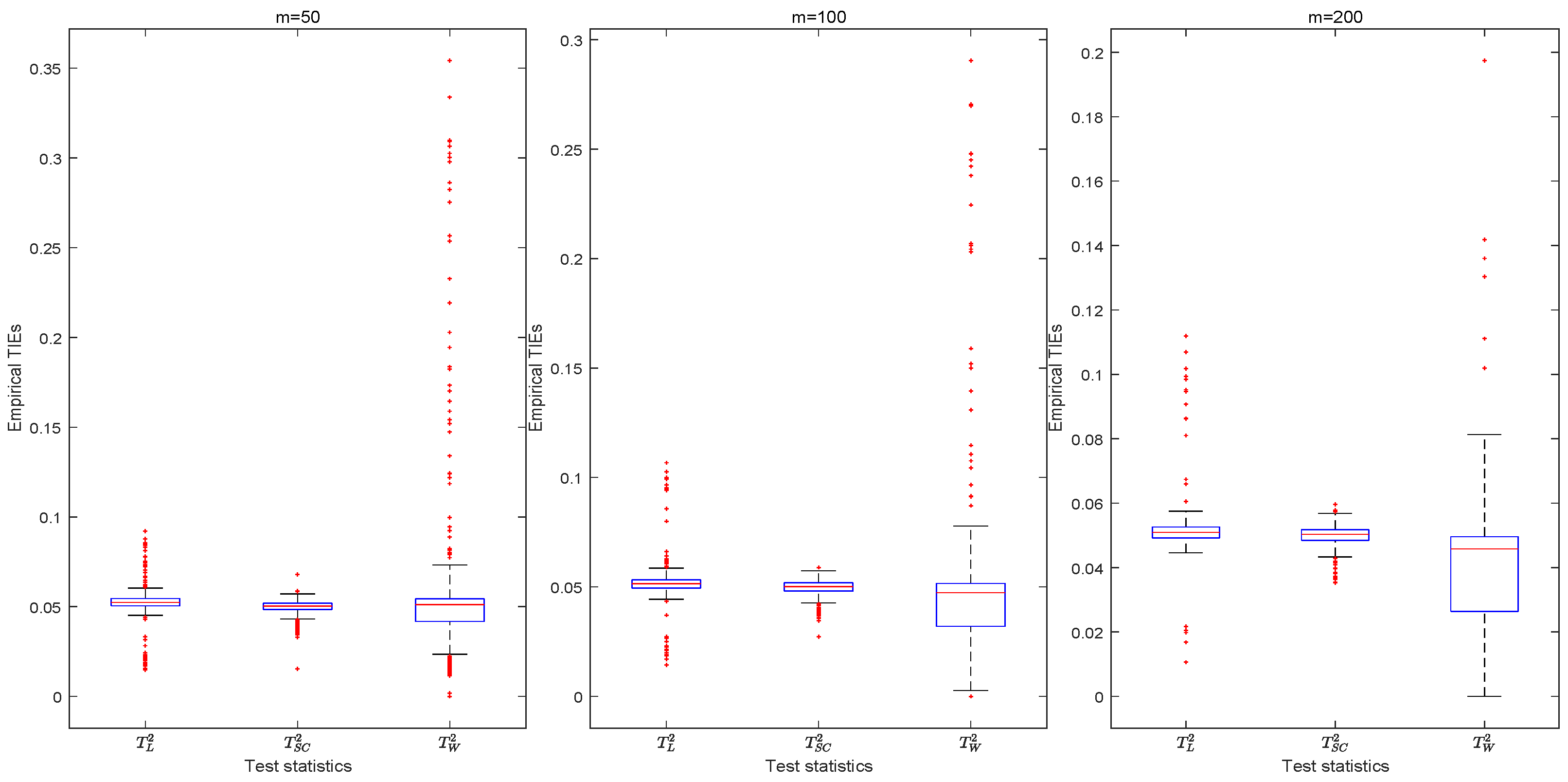
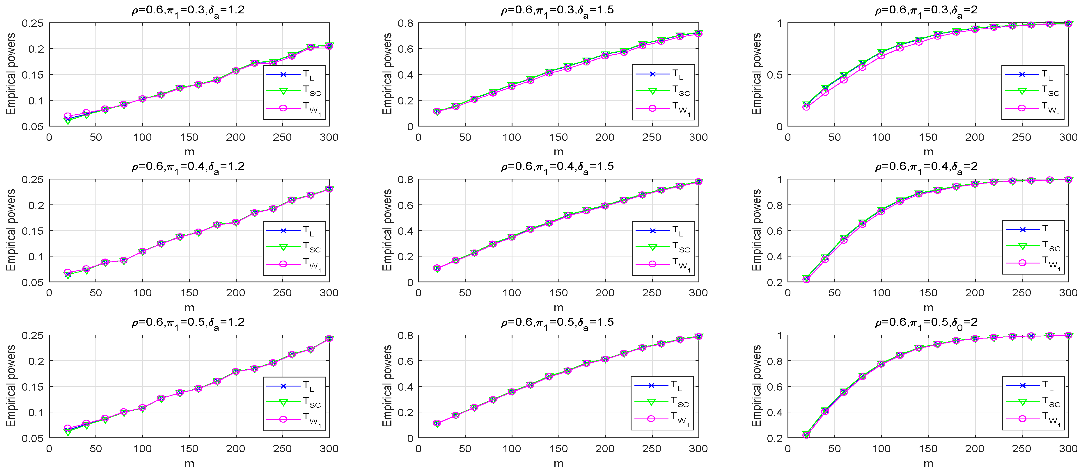
6.1. Odds Ratio Test

In this subsection, we investigate the performance of various test statistics for the odds ratio $\delta$ in terms of the behaviors of empirical type I error rates (TIEs) and empirical powers. 10,000 replicates are randomly generated from the null hypothesis $H_0$ or alternative $H_a$ for each configuration. The empirical TIEs of test $T(=T_L^2,T_S^2,T_W^2)$ at a nominal level $\alpha$ are computed by dividing the number of times that the null hypothesis is rejected by 10,000 replicates that come from the null hypothesis $H_0$. Following Cochran [28] and Tang et al. [11], a test at a nominal level 0.05 is said to be liberal if the empirical TIE is greater than 0.06; conservative if the TIE is less than 0.04; and robust if the TIE is between 0.04 and 0.06.

Under the parameter settings: $\rho =0.4,0.6,0.8$, ${\pi }_1=0.2,0.4,0.6$ and $m\triangleq m_{+1}=m_{+2}=50,75,100$, and

Table 2. Empirical TIEs of tests under $H_0:{\delta }_0=1,1.5,2$.

$\mathit{\rho }$	${\mathit{\pi }}_1$	${\mathit{\delta }}_0$	$\mathit{m}=50$			$\mathit{m}=75$			$\mathit{m}=100$
			${\mathit{T}}_{\mathit{L}}^{\mathbf{2}}$	${\mathit{T}}_{\mathit{S}}^{\mathbf{2}}$	${\mathit{T}}_{\mathit{W}}^{\mathbf{2}}$	${\mathit{T}}_{\mathit{L}}^{\mathbf{2}}$	${\mathit{T}}_{\mathit{S}}^{\mathbf{2}}$	${\mathit{T}}_{\mathit{W}}^{\mathbf{2}}$	${\mathit{T}}_{\mathit{L}}^{\mathbf{2}}$	${\mathit{T}}_{\mathit{S}}^{\mathbf{2}}$	${\mathit{T}}_{\mathit{W}}^{\mathbf{2}}$
	0.2	1.0	0.0548	0.0527	0.0586	0.0513	0.0496	0.0533	0.0551	0.0546	0.0570
		1.5	0.0530	0.0514	0.0521	0.0507	0.0492	0.0468	0.0512	0.0494	0.0471
		2.0	0.0485	0.0470	0.0408	0.0522	0.0511	0.0422	0.0492	0.0481	0.0386
	0.4	1.0	0.0538	0.0524	0.0548	0.0529	0.0521	0.0542	0.0511	0.0501	0.0519
0.4		1.5	0.0484	0.0474	0.0498	0.0509	0.0509	0.0511	0.0504	0.0498	0.0513
		2.0	0.0481	0.0474	0.0494	0.0513	0.0502	0.0517	0.0540	0.0526	0.0546
	0.6	1.0	0.0543	0.0526	0.0555	0.0517	0.0509	0.0526	0.0498	0.0495	0.0503
		1.5	0.0512	0.0502	0.0513	0.0476	0.0471	0.0467	0.0498	0.0493	0.0485
		2.0	0.0508	0.0495	0.0464	0.0505	0.0502	0.0437	0.0497	0.0496	0.0440
	0.2	1.0	0.0540	0.0522	0.0594	0.0509	0.0492	0.0544	0.0522	0.0508	0.0543
		1.5	0.0532	0.0520	0.0525	0.0504	0.0493	0.0472	0.0509	0.0504	0.0481
		2.0	0.0487	0.0462	0.0404	0.0509	0.0491	0.0408	0.0514	0.0501	0.0405
	0.4	1.0	0.0519	0.0507	0.0540	0.0500	0.0492	0.0513	0.0502	0.0495	0.0512
0.6		1.5	0.0499	0.0485	0.0515	0.0514	0.0511	0.0522	0.0526	0.0519	0.0529
		2.0	0.0496	0.0483	0.0518	0.0521	0.0511	0.0515	0.0508	0.0516	0.0511
	0.6	1.0	0.0525	0.0510	0.0543	0.0517	0.0512	0.0530	0.0503	0.0499	0.0516
		1.5	0.0484	0.0469	0.0489	0.0525	0.0515	0.0513	0.0480	0.0475	0.0472
		2.0	0.0524	0.0500	0.0468	0.0498	0.0496	0.0444	0.0512	0.0511	0.0453
	0.2	1.0	0.0533	0.0505	0.0607	0.0533	0.0518	0.0572	0.0522	0.0508	0.0544
		1.5	0.0552	0.0530	0.0544	0.0527	0.0515	0.0511	0.0493	0.0485	0.0467
		2.0	0.0496	0.0477	0.0422	0.0520	0.0507	0.0448	0.0544	0.0536	0.0442
	0.4	1.0	0.0500	0.0493	0.0522	0.0496	0.0491	0.0508	0.0498	0.0495	0.0509
0.8		1.5	0.0527	0.0519	0.0533	0.0509	0.0505	0.0523	0.0557	0.0550	0.0556
		2.0	0.0532	0.0523	0.0564	0.0526	0.0540	0.0537	0.0514	0.0525	0.0522
	0.6	1.0	0.0528	0.0517	0.0557	0.0526	0.0520	0.0536	0.0524	0.0522	0.0531
		1.5	0.0504	0.0489	0.0518	0.0520	0.0509	0.0520	0.0534	0.0525	0.0533
		2.0	0.0532	0.0514	0.0511	0.0511	0.0522	0.0445	0.0514	0.0521	0.0460

provides the empirical TIEs of various tests for $H_0:{\delta }_0=1,1.5,2$ at a nominal level $\alpha =0.05$, respectively. In the table, if the value of the corresponding TIE is less than 0.04, or greater than 0.06, it is highlighted in bold. We observe that the empirical TIEs of the likelihood ratio and score tests are closer to 0.05. Thus, these two tests are more robust than the Wald-type test for the specific parameter settings. To further compare the three test statistics, we randomly choose 1000 parameter settings: $\rho \in (0,1)$, ${\pi }_i\in (0,1)(i=1,2)$, and $m=50,100,200$. In Figure 1, a set of boxplots shows the distribution for the empirical TIEs for tests $T_L^2,T_{SC}^2,T_W^2$, respectively. Among these tests, the score test is the most robust because its TIEs are closer to the pre-specified nominal level of 0.05, followed by the likelihood ratio test. However, the Wald-type test is liberal or conservative under certain conditions. Thus, the score test is recommended based on empirical TIEs.

We evaluate the empirical powers of the three proposed test statistics by the percentage of rejecting $H_0$ with 10,000 replicates that come from the alternative hypothesis $H_a$. Under $H_0:\delta =1 \mathrm{vs}. H_a:{\delta }_a=1.2,1.5,2$ at $\alpha =0.05$, we still use the parameter settings $\rho =0.4,0.6,0.8$, ${\pi }_1=0.2,0.4,0.6$ and $m=50,75,100$.

Table 3. Empirical powers of tests under $H_0:{\delta }_0=1$ vs. $H_a:{\delta }_a=1.2,1.5,2$.

$\mathit{\rho }$	${\mathit{\pi }}_1$	${\mathit{\delta }}_{\mathit{a}}$	$\mathit{m}=50$			$\mathit{m}=75$			$\mathit{m}=100$
			${\mathit{T}}_{\mathit{L}}^{\mathbf{2}}$	${\mathit{T}}_{\mathit{S}}^{\mathbf{2}}$	${\mathit{T}}_{\mathit{W}}^{\mathbf{2}}$	${\mathit{T}}_{\mathit{L}}^{\mathbf{2}}$	${\mathit{T}}_{\mathit{S}}^{\mathbf{2}}$	${\mathit{T}}_{\mathit{W}}^{\mathbf{2}}$	${\mathit{T}}_{\mathit{L}}^{\mathbf{2}}$	${\mathit{T}}_{\mathit{S}}^{\mathbf{2}}$	${\mathit{T}}_{\mathit{W}}^2$
	0.2	1.2	0.0749	0.0741	0.0768	0.0837	0.0831	0.0834	0.1056	0.1057	0.1036
		1.5	0.1702	0.1720	0.1522	0.2399	0.2439	0.2141	0.2846	0.2886	0.2591
		2.0	0.3854	0.3941	0.2991	0.5362	0.5458	0.4463	0.6566	0.6654	0.5696
	0.4	1.2	0.0859	0.0851	0.0862	0.0983	0.0979	0.0981	0.1205	0.1203	0.1199
0.4		1.5	0.2147	0.2158	0.2101	0.3190	0.3212	0.3125	0.3920	0.3939	0.3849
		2.0	0.5164	0.5216	0.4964	0.6908	0.6954	0.6742	0.8183	0.8214	0.8067
	0.6	1.2	0.0855	0.0850	0.0859	0.1007	0.1007	0.1000	0.1226	0.1223	0.1220
		1.5	0.2188	0.2201	0.2135	0.3152	0.3169	0.3084	0.3858	0.3879	0.3788
		2.0	0.5193	0.5242	0.4984	0.6957	0.6999	0.6809	0.8145	0.8173	0.8042
	0.2	1.2	0.0718	0.0707	0.0748	0.0770	0.0765	0.0777	0.0967	0.0962	0.0960
		1.5	0.1552	0.1575	0.1401	0.2133	0.2168	0.1923	0.2566	0.2606	0.2302
		2.0	0.3449	0.3544	0.2607	0.4828	0.4932	0.3942	0.6006	0.6100	0.5140
	0.4	1.2	0.0845	0.0836	0.0850	0.0915	0.0911	0.0915	0.1152	0.1152	0.1154
0.6		1.5	0.1976	0.1988	0.1930	0.2826	0.2844	0.2769	0.3503	0.3516	0.3424
		2.0	0.4656	0.4714	0.4457	0.6384	0.6430	0.6185	0.7607	0.7643	0.7456
	0.6	1.2	0.0854	0.0842	0.0866	0.0936	0.0929	0.0935	0.1164	0.1162	0.1160
		1.5	0.1908	0.1913	0.1863	0.2825	0.2838	0.2760	0.3495	0.3513	0.3433
		2.0	0.4654	0.4729	0.4452	0.6350	0.6425	0.6163	0.7626	0.7675	0.7493
	0.2	1.2	0.0695	0.0679	0.0731	0.0751	0.0747	0.0768	0.0926	0.0925	0.0932
		1.5	0.1403	0.1427	0.1276	0.1941	0.1974	0.1724	0.2305	0.2342	0.2097
		2.0	0.3112	0.3239	0.2377	0.4344	0.4457	0.3500	0.5510	0.5605	0.4567
	0.4	1.2	0.0771	0.0766	0.0785	0.0859	0.0856	0.0868	0.1025	0.1023	0.1024
0.8		1.5	0.1816	0.1827	0.1786	0.2417	0.2440	0.2372	0.3186	0.3210	0.3136
		2.0	0.4328	0.4378	0.4141	0.5952	0.6012	0.5769	0.7183	0.7242	0.7031
	0.6	1.2	0.0792	0.0783	0.0809	0.0887	0.0886	0.0894	0.1052	0.1052	0.1054
		1.5	0.1838	0.1849	0.1808	0.2459	0.2478	0.2399	0.3180	0.3204	0.3117
		2.0	0.4282	0.4350	0.4070	0.5946	0.6019	0.5750	0.7178	0.7256	0.7004

displays the empirical powers of $T_L^2,T_S^2$ and $T_W^2$ under the given settings. The power values of the three tests increase when the sample size m or ${\delta }_a$ increases. Given $\rho ,{\pi }_1,{\delta }_a$ and m, if the power is the largest in the table, it is highlighted in bold. Compared with these tests, the largest powers are mostly found in the score test, the Wald-type test, and the likelihood ratio test. On the other hand, we chose some new settings of parameters to illustrate the powers of the above tests: $\rho =0.6$ and ${\pi }_1=0.3,0.4,0.5$ for $m=20,40,...,300$ under $H_0:{\delta }_0=1$ and $H_a:{\delta }_a=1.2,1.5,2$. Figure 2 shows the trajectories of empirical powers for our proposed tests $T_L^2,T_{SC}^2$ and $T_W^2$. As expected, the empirical powers of all tests are larger as the sample size m increases. Moreover, we observed that the powers of the likelihood ratio and the score tests are close, but the Wald-type test has lower power under specific conditions.

Overall, the score test is more robust with a higher power than the likelihood ratio and the Wald-type tests. Therefore, the score statistic is recommended for testing whether the odds ratio $\delta$ of response rates is equal to a specific value ${\delta }_0$.

6.2. CI Construction

In this subsection, we compared the four CI methods through the empirical mean coverage probability (MCP) and empirical mean interval width (MIW). Under $H_0$, the MCP is defined as the proportions of samples that true odds ratio $\delta$ falls within the constructed CI, and the MIW is computed by dividing the sum of all widths by the total number of replicates. For the observed data $\mathbf{m}$, let ${\delta }_U\left(\mathbf{m}\right)$ and ${\delta }_L\left(\mathbf{m}\right)$ be the estimators of the CI lower limit and upper limit of ${\delta }_0$, respectively. The formula of MCP and MIW is expressed by

$$\begin{array}{ccc}& & MCP=\frac{1}{N}\sum _{k=1}^{N}I\{{\delta }_0\in [{\delta }_L({\mathbf{m}}^{\left(k\right)},{\delta }_U({\mathbf{m}}^{\left(k\right)})]\},\hfill \\ & & MIW=\frac{1}{N}\sum _{k=1}^N[{\delta }_U({\mathbf{m}}^{\left(k\right)})-{\delta }_L({\mathbf{m}}^{\left(k\right)}],\hfill \end{array}$$

where ${\mathbf{m}}^{\left(k\right)}$ is the kth sample in the bilateral design, and $I(·)$ is an indicator function. Here, the number of replicates $N$ = 10,000.

We consider the exact sample sizes and parameter setups for calculating the empirical TIE and power. Ten thousand replicates are generated from a trinomial distribution for each configuration, upon which MCP and MIW are computed. We list the performance of four CI methods in

Table 4. MCPs and MIWs of CI methods.

$\mathit{\rho }$	${\mathit{\pi }}_1$	${\mathit{\delta }}_0$	m	MCPs				MIWs
				${\mathit{CI}}_{\mathit{L}}$	${\mathit{CI}}_{\mathit{S}}$	${\mathit{CI}}_{{\mathit{W}}_{\mathbf{1}}}$	${\mathit{CI}}_{{\mathit{W}}_{\mathbf{2}}}$	${\mathit{CI}}_{\mathit{L}}$	${\mathit{CI}}_{\mathit{S}}$	${\mathit{CI}}_{{\mathit{W}}_{\mathbf{1}}}$	${\mathit{CI}}_{{\mathit{W}}_{\mathbf{2}}}$
	0.2	1.0	50	0.9493	0.9523	0.9830	0.9452	2.0316	1.9674	2.1187	5.5245
			75	0.9453	0.9466	0.9704	0.9423	1.5344	1.5018	1.5711	2.9333
			100	0.9442	0.9448	0.9649	0.9425	1.2713	1.2512	1.2923	1.7555
		1.5	50	0.9475	0.9492	0.9745	0.9492	2.9290	2.8005	3.1746	8.2801
			75	0.9449	0.9463	0.9654	0.9479	2.2036	2.1224	2.3304	4.8852
			100	0.9460	0.9467	0.9624	0.9488	1.8224	1.7568	1.9075	2.9070
		2.0	50	0.9472	0.9501	0.9726	0.9555	3.8250	3.5607	4.3147	10.725
			75	0.9456	0.9464	0.9680	0.9539	2.8792	2.6584	3.1555	6.7246
			100	0.9453	0.9460	0.9645	0.9566	2.3808	2.1818	2.5795	4.1505
	0.4	1.0	50	0.9485	0.9496	0.9518	0.9473	1.5394	1.5225	1.5367	1.6188
			75	0.9468	0.9474	0.9488	0.9460	1.1985	1.1902	1.1969	1.2290
			100	0.9458	0.9469	0.9479	0.9451	1.0129	1.0080	1.0119	1.0303
		1.5	50	0.9481	0.9493	0.9499	0.9472	2.3032	2.2362	2.3022	2.4288
0.4			75	0.9448	0.9458	0.9462	0.9451	1.7860	1.7360	1.7889	1.8407
			100	0.9473	0.9479	0.9489	0.9469	1.5066	1.4641	1.5100	1.5401
		2.0	50	0.9478	0.9487	0.9498	0.9473	3.1016	2.9648	3.1195	3.3004
			75	0.9449	0.9456	0.9458	0.9452	2.3874	2.2899	2.4076	2.4824
			100	0.9447	0.9442	0.9451	0.9442	2.0080	1.9323	2.0304	2.0740
	0.6	1.0	50	0.9477	0.9503	0.9534	0.9463	1.5410	1.5188	1.5399	1.6211
			75	0.9479	0.9485	0.9498	0.9470	1.1945	1.1820	1.1943	1.2265
			100	0.9475	0.9479	0.9493	0.9468	1.0104	1.0025	1.0103	1.0287
		1.5	50	0.9686	0.9694	0.9779	0.9568	2.3816	2.3061	2.4202	3.0219
			75	0.9488	0.9497	0.9541	0.9496	1.8622	1.8107	1.8940	2.0624
			100	0.9447	0.9448	0.9505	0.9453	1.5702	1.5296	1.5959	1.6858
		2.0	50	0.9522	0.9507	0.9542	0.9504	3.3840	3.3309	3.4267	3.6675
			75	0.9488	0.9436	0.9502	0.9470	2.6095	2.5402	2.6397	2.7368
			100	0.9508	0.9421	0.9623	0.9421	2.1988	2.1379	2.3058	2.1379
	0.2	1.0	50	0.9499	0.9522	0.9897	0.9450	2.2557	2.1620	2.3876	7.2516
			75	0.9428	0.9447	0.9747	0.9388	1.6813	1.6380	1.7318	4.0515
			100	0.9475	0.9488	0.9693	0.9455	1.3810	1.3539	1.4082	2.2598
		1.5	50	0.9505	0.9526	0.9777	0.9519	3.2400	3.0097	3.5806	10.147
			75	0.9439	0.9454	0.9684	0.9473	2.4165	2.2439	2.5794	6.4631
			100	0.9457	0.9467	0.9653	0.9490	1.9799	1.8306	2.0828	3.8025
		2.0	50	0.9473	0.9496	0.9731	0.9550	4.2432	3.6543	4.9050	12.504
			75	0.9438	0.9453	0.9681	0.9543	3.1368	2.6729	3.4960	8.4027
			100	0.9455	0.9465	0.9660	0.9559	2.5611	2.1940	2.8188	5.3252
	0.4	1.0	50	0.9484	0.9497	0.9535	0.9471	1.6799	1.6372	1.6812	1.7960
			75	0.9465	0.9472	0.9488	0.9438	1.2961	1.2737	1.2967	1.3371
			100	0.9454	0.9460	0.9481	0.9446	1.0922	1.0775	1.0926	1.1152
		1.5	50	0.9485	0.9499	0.9524	0.9474	2.4973	2.3678	2.5249	2.6951
0.6			75	0.9463	0.9472	0.9480	0.9452	1.9173	1.8280	1.9388	2.0037
			100	0.9471	0.9474	0.9484	0.9468	1.6092	1.5373	1.6314	1.6683
		2.0	50	0.9491	0.9499	0.9514	0.9483	3.3828	3.2200	3.4235	3.6697
			75	0.9480	0.9477	0.9496	0.9470	2.5817	2.4907	2.6138	2.7080
			100	0.9455	0.9446	0.9465	0.9444	2.1741	2.1157	2.1988	2.2527
	0.6	1.0	50	0.9521	0.9530	0.9573	0.9500	1.6774	1.6321	1.6835	1.7933
			75	0.9471	0.9471	0.9503	0.9465	1.2904	1.2657	1.2941	1.3347
			100	0.9494	0.9494	0.9515	0.9483	1.0904	1.0734	1.0936	1.1162
		1.5	50	0.9508	0.9500	0.9568	0.9587	2.5422	2.4373	2.5845	3.1324
			75	0.9483	0.9488	0.9544	0.9483	2.0101	1.9410	2.0545	2.2830
			100	0.9474	0.9477	0.9535	0.9481	1.6926	1.6416	1.7286	1.8467
		2.0	50	0.9498	0.9509	0.9677	0.9435	3.8470	3.6810	4.1480	4.3245
			75	0.9462	0.9426	0.9619	0.9534	2.8526	2.7697	3.0117	3.4562
			100	0.9552	0.9417	0.9686	0.9579	2.3734	2.3234	2.4872	2.9232
	0.2	1.0	50	0.9528	0.9555	0.9922	0.9464	2.5289	2.3713	2.7335	8.7236
			75	0.9463	0.9479	0.9783	0.9425	1.8500	1.7662	1.9150	5.3330
			100	0.9475	0.9490	0.9715	0.9445	1.5029	1.4441	1.5372	3.0518
		1.5	50	0.9501	0.9527	0.9787	0.9490	3.6306	3.1170	4.1349	11.568
			75	0.9446	0.9460	0.9705	0.9472	2.6451	2.2278	2.8486	7.9263
			100	0.9464	0.9472	0.9660	0.9507	2.1423	1.7948	2.2715	4.9722
		2.0	50	0.9491	0.9510	0.9746	0.9551	4.6967	3.5029	5.6867	13.775
			75	0.9450	0.9468	0.9689	0.9552	3.3559	2.5244	3.8704	9.9300
			100	0.9454	0.9455	0.9674	0.9549	2.6568	2.0836	3.0760	6.6606
	0.4	1.0	50	0.9500	0.9507	0.9560	0.9478	1.8165	1.7262	1.8307	2.0030
			75	0.9453	0.9455	0.9488	0.9434	1.3881	1.3349	1.3975	1.4489
			100	0.9473	0.9475	0.9492	0.9462	1.1663	1.1254	1.1726	1.2006
		1.5	50	0.9467	0.9485	0.9510	0.9454	2.6973	2.5073	2.7506	2.9965
0.8			75	0.9471	0.9475	0.9493	0.9457	2.0383	1.9086	2.0880	2.1704
			100	0.9447	0.9453	0.9465	0.9445	1.7059	1.6064	1.7512	1.7970
		2.0	50	0.9510	0.9520	0.9543	0.9487	3.6860	3.4993	3.7225	4.0628
			75	0.9460	0.9441	0.9469	0.9449	2.7847	2.6841	2.8147	2.9357
			100	0.9457	0.9435	0.9469	0.9456	2.3368	2.2760	2.3590	2.4272
	0.6	1.0	50	0.9501	0.9512	0.9564	0.9462	1.8097	1.7452	1.8189	1.9620
			75	0.9483	0.9486	0.9522	0.9466	1.3874	1.3450	1.3960	1.4484
			100	0.9468	0.9472	0.9498	0.9461	1.1667	1.1337	1.1736	1.2018
		1.5	50	0.9481	0.9494	0.9614	0.9624	2.9340	2.8031	3.0144	3.3773
			75	0.9471	0.9476	0.9546	0.9512	2.1868	2.1098	2.2356	2.5099
			100	0.9490	0.9498	0.9558	0.9501	1.8275	1.7677	1.8656	2.0184
		2.0	50	0.9478	0.9495	0.9684	0.9623	4.2564	4.0509	4.6223	3.3772
			75	0.9483	0.9404	0.9639	0.9512	3.1063	3.0129	3.2850	2.5099
			100	0.9483	0.9400	0.9612	0.9501	2.5767	2.5198	2.7035	2.0184

. In the table, if the value of MCPs is less than 0.94, or greater than 0.96, then it is bold. We observed that the MCPs of $C{I}_L$, $C{I}_S$, and $C{I}_{W_2}$ are close to the confidence level of 0.95. Some MCPs of the $C{I}_{W_1}$ method are slightly conservative, i.e., slightly above 0.95. On the other hand, the $C{I}_S$ method has the shortest MIWs, followed by $C{I}_L$, then $C{I}_{W_2}$ and $C{I}_{W_2}$. Although the $C{I}_{W_1}$ method is slightly more conservative than $C{I}_{W_2}$, it has shorter MIWs than $C{I}_{W_2}$. The result reveals that the bisection root-finding algorithm is more effective than the asymptotic normality method in constructing the interval.

In conclusion, the $C{I}_S$ method performs better with the satisfactory MCPs and the shortest MIWs among the proposed methods. Thus, the CI method based on the score statistic is recommended to construct the interval of odds ratio ${\delta }_0$.

7. An Example

Mandel et al. (1982) conducted a double-blinded randomized clinical trial at two sites comparing cefaclor and amoxicillin for the treatment of acute otitis media with effusion (OME) in 214 children (293 ears). Each child underwent bilateral tympanocentesis and was randomly assigned to receive a 14-day course of either cefaclor or amoxicillin.

Table 5. OME status after 14-day course of antibiotic treatment.

OME Status	Treatment		Total
	Cefaclor	Amoxicillin
None cured	14	15	29
Unilateral cured	9	3	12
Bilateral cured	21	13	34
Total	44	31	75

shows the OME status at 14 days in 75 children with bilateral OME. In this section, the real example was used to illustrate the performance of our proposed test statistics and CI methods (Table 5). According to Table 5, we have $m_{01}=14,m_{11}=9,m_{21}=21,$$m_{02}=15,m_{12}=3,m_{22}=13$ and $m_{+1}=44,m_{+2}=31$. At a nominal level $\alpha =0.05$, we have ${\chi }_{1,1-\alpha }^2={\chi }_{1,0.95}^2=3.8415$ and $z_{1-\alpha /2}=z_{0.975}=1.96$.

We first tested whether the two cured rates of cefaclor and amoxicillin are clinically equal; that is, $H_0:\delta =1$ vs. $H_a:\delta \ne 1$. Under the alternative hypothesis $H_a$, the unconstrained MLEs of $\rho$ and ${\pi }_i(i=1,2)$ are $\hat{\rho }=0.6747,{\widehat{\pi }}_1=0.5767$ and ${\widehat{\pi }}_2=0.4660$. The constrained MLEs under null hypothesis $H_0$ are $\tilde{\rho }=0.6786,{\tilde{\pi }}_1={\tilde{\pi }}_2=0.5333$. The result reveals that there exists a correlation between the two ears of a patient. Under $H_0$, the values of the three proposed test statistics are $T_L^2=1.0505,T_S^2=1.0305$ and $T_W^2=1.0717$, and the corresponding p-value $p=0.3054,0.3100,0.3006$. Since $T_L^2,T_S^2,T_W^2<{\chi }_{1,0.95}^2$ and $p>0.05$, we failed to reject the null hypothesis $H_0$ at the significance level $\alpha =0.05$. Thus, there are no significant differences between cefaclor and amoxicillin.

Applying the proposed CI procedures, we then obtained four pairs of confidence limits:

$$\begin{array}{ccc}& & [\mathrm{LL},\mathrm{LU}]=[0.2702,1.5026],[{\mathrm{WL}}_1,{\mathrm{WU}}_1]=[0.2739,1.4974],\hfill \\ & & [\mathrm{SL},\mathrm{SU}]=[0.2727,1.5087],[{\mathrm{WL}}_2,{\mathrm{WU}}_2]=[0.2638,1.4939].\hfill \end{array}$$

The confidence limits contain 1. There are no significant differences between the two antibiotic treatments based on our proposed tests and CI methods. Through the example, we note that the same conclusions can explain with test statistics and CI methods. In addition, the CI methods contain more information than the hypothesis test.

8. Conclusions

In this paper, we proposed three test statistics for testing the odds ratio of two proportions and constructed four pairs of CIs for the ratio. Under an alternative hypothesis, we obtain the unconstrained MLEs by an iteration procedure through two steps. The constrained MLEs under the null hypothesis was given based on the Fisher scoring algorithm. Given the MLEs, the likelihood ratio test, the score test, and the Wald-type log-linear test were proposed, which asymptotically followed a chi-square distribution with one degree of freedom. Four CIs of the odds ratio of two proportions were based on inverting the three test statistics, including CI based on a likelihood ratio statistic, CI based on a score test, and two CI methods based on the Wald-type test. The bisection root-finding algorithm was used to search for the profile likelihood, Wald-type, score CI upper and lower limits of odds ratios. The asymptotic normality method obtained other CI upper and lower limits of the Wald-type case. We conducted simulation studies to compare the proposed tests about the empirical type I error, power, and CI methods in terms of the MCPs and MIEs. The results revealed that the score test performed better than other statistics, and the CI based on score statistic is recommended. A real example was provided to illustrate our results.

One of the possible future works is to extend these test statistics and CI methods to general $g(g\ge 2)$ cases for bilateral correlated data.

References

1. Lewis, T.L.; Maurer, D.; Brent, H. Development of grating acuity in children treated for unilateral or bilateral congenital cataract. Investig. Ophthalmol. Vis. Sci. 1995, 36, 2080–2095. [Google Scholar]
2. Pompeo, E.; Sergiacomi, G.; Nofroni, I.; Roscetti, W.; Simonetti, G.; Mineo, T.C. Morphologic grading of emphysema is useful in the selection of candidates for unilateral or bilateral reduction pneumoplasty. Eur. J.-Cardio-Thorac. Surg. 2000, 17, 680–686. [Google Scholar] [CrossRef]
3. Brwon, M.M.; Brown, G.C.; Sharma, S.; Busbee, B.; Brown, H. Quality of life associated with unilateral and bilateral good vision. Ophthalmology 2001, 108, 643–648. [Google Scholar] [CrossRef]
4. Newman, L.A.; Sahin, A.A.; Bondy, M.L.; Mirza, N.Q.; Vlastos, G.S.; Whitman, G.J.; Buchholz, T.A.; Lee, M.H.; Singletary, S.E. A case-control study of unilateral and bilateral breast carcinoma patients. Cancer 2001, 91, 1845–1853. [Google Scholar] [CrossRef]
5. Mandel, E.M.; Bluestone, C.D.; Rockette, H.E.; Blatter, M.M.; Reisinger, K.S.; Wucher, F.P.; Harper, J. Duration of effusion after antibiotic treatment for acute otitis media: Comparison of cefaclor and amoxicillin. Pediatr. Infect. Dis. 1982, 1, 310–316. [Google Scholar] [CrossRef]
6. Sainani, K. The importance of accounting for correlated observations. Am. Acad. Phys. Med. Rehabil. 2010, 2, 858–861. [Google Scholar] [CrossRef] [PubMed]
7. Cessie, S.L.; Houwelingen, J.C. Logistic regression for correlated binary data. Appl. Stat. 1994, 43, 95–108. [Google Scholar] [CrossRef]
8. Ying, G.; Maguire, M.G.; Glynn, R.; Rosner, B. Tutorial on biostatistics: Linear regression analysis of continuous correlated eye data. Ophthalmic Epidemiol. 2017, 24, 130–140. [Google Scholar] [CrossRef]
9. Rosner, B. Statistical methods in ophthalmology: An adjustment for the intraclass correlation between eyes. Biometrics 1982, 38, 105–114. [Google Scholar] [CrossRef]
10. Ma, C.X.; Shan, G.; Liu, S. Homogeneity test for binary correlated data. PLoS ONE 2015, 10, e0124337. [Google Scholar] [CrossRef]
11. Tang, M.L.; Tang, N.S.; Rosner, B. Statistical inference for correlated data in ophthalmologic studies. Stat. Med. 2006, 25, 2771–2783. [Google Scholar] [CrossRef] [PubMed]
12. Tang, N.S.; Qiu, S.F.; Tang, M.L.; Pei, Y.B. Asymptotic confidence interval construction for proportion difference in medical studies with bilateral data. Stat. Meth. Med. Res. 2011, 20, 233–259. [Google Scholar] [CrossRef] [PubMed]
13. Dallal, G.E. Paired Bernoulli trials. Biometrics 1988, 44, 253–257. [Google Scholar] [CrossRef]
14. Sun, S.M.; Li, Z.M.; Ai, M.Y.; Jiang, H.J. Risk difference tests for stratified binary data under Dallal’s model. Stat. Meth. Med. Res. 2022, 31, 1135–1156. [Google Scholar] [CrossRef]
15. Donner, A. Statistical methods in opthalmology: An adjusted chi-square approach. Biometrics 1989, 45, 605–611. [Google Scholar] [CrossRef] [PubMed]
16. Liu, X.B.; Liu, S.; Ma, C.X. Testing equality of correlation coefficients for paired binary data from multiple groups. Stat. Compu. Simul. 2015, 86, 1686–1696. [Google Scholar] [CrossRef]
17. Pei, Y.B.; Tang, M.L.; Wong, W.K.; Guo, J.H. Confidence intervals for correlated proportion differences from paired data in a two-arm randomised clinical trial. Stat. Meth. Med. Res. 2010, 21, 167–187. [Google Scholar] [CrossRef] [PubMed]
18. Pei, Y.B.; Tian, G.L.; Tang, M.L. Testing homogeneity of proportion ratios for stratified correlated bilateral data in two-arm randomized clinical trials. Stat. Med. 2014, 33, 4370–4386. [Google Scholar] [CrossRef]
19. Qiu, S.F.; Tang, N.S.; Tang, M.L.; Pei, Y.B. Sample Size for testing difference between two proportions for the bilateral-sample design. J. Biopharm. Stat. 2009, 19, 857–871. [Google Scholar] [CrossRef]
20. Qiu, S.F.; Liu, Q.S.; Ge, Y. Confidence intervals of proportion differences for stratified combined unilateral and bilateral data. Commun. Stat. Simul. Comp. 2021. [Google Scholar] [CrossRef]
21. Tang, N.S.; Tang, M.L.; Qiu, S.F. Testing the equality of proportions for correlated otolaryngologic data. Comput. Stat. Data Anal. 2008, 52, 3719–3729. [Google Scholar] [CrossRef]
22. Tang, N.S.; Li, H.Q.; Tang, M.L.; Li, J. Confidence interval construction for the difference between two correlated proportions with missing observations. J. Biopharm. Stat. 2016, 26, 323–338. [Google Scholar] [CrossRef] [PubMed]
23. Tang, M.L.; Pei, Y.B.; Wong, W.K.; Li, J.L. Goodness-of-fit tests for correlated paired binary data. Stat. Methods Med. Res. 2010, 21, 331–345. [Google Scholar] [CrossRef] [PubMed]
24. Edwards, A.W.F. The measure of association in a 2 × 2 table. J. Roy. Stat. Soc. A Stat. 1963, 126, 109–114. [Google Scholar] [CrossRef]
25. Chanda, K.C. A Note on the Consistency and Maxima of the Roots of Likelihood Equations. Biometrika 1954, 41, 56–61. [Google Scholar] [CrossRef]
26. Mou, K.Y.; Li, Z.M. Homogeneity test of many-to-one risk differences for correlated binary data under optimal algorithms. Complexity 2021, 2021, 6685951. [Google Scholar] [CrossRef]
27. Ma, C.X.; Liu, S. Testing equality of proportions for correlated binary data in ophthalmologic studies. J. Biopharm. Stat. 2017, 27, 611–619. [Google Scholar] [CrossRef]
28. Cochran, W.G. The χ2 test of goodness of fit. Anal. Math. Stat. 1952, 23, 315–345. [Google Scholar] [CrossRef]
Figure 1. Boxplots of empirical TIEs for 1000 parameter settings.
Axioms 11 00502 g001
Figure 2. Curves of empirical powers under H 0 : δ 0 = 1 .
Axioms 11 00502 g002