Article

A New 3-Parameter Bounded Beta Distribution: Properties, Estimation, and Applications

by
Faiza A. Althubyani
1,
Ahmed M. T. Abd El-Bar
1,2,*,
Mohamad A. Fawzy
1,3 and
Ahmed M. Gemeay
2
1
Department of Mathematics, College of Science, Taibah University, Al-Madina 41411, Saudi Arabia
2
Department of Mathematics, Faculty of Science, Tanta University, Tanta 31527, Egypt
3
Department of Mathematics, Faculty of Science, Suez University, Suez 43111, Egypt
*
Author to whom correspondence should be addressed.
Axioms 2022, 11(10), 504; https://doi.org/10.3390/axioms11100504
Submission received: 11 August 2022 / Revised: 5 September 2022 / Accepted: 13 September 2022 / Published: 26 September 2022
(This article belongs to the Special Issue Computational Statistics & Data Analysis)

Abstract

:
This study presents a new three-parameter beta distribution defined on the unit interval, which can have increasing, decreasing, left-skewed, right-skewed, approximately symmetric, bathtub, and upside-down bathtub shaped densities, and increasing, U, and bathtub shaped hazard rates. This model can define well-known distributions with various parameters and supports, such as Kumaraswamy, beta exponential, exponential, exponentiated exponential, uniform, the generalized beta of the first kind, and beta power distributions. We present a comprehensive account of the mathematical features of the new model. Maximum likelihood methods and a Bayesian method under squared error and linear exponential loss functions are presented; also, approximate confidence intervals are obtained. We present a simulation study to compare all the results. Two real-world data sets are analyzed to demonstrate the utility and adaptability of the proposed model.

1. Introduction

The beta distribution is a well-known distribution often used to model and analyze lifetime data because it has exciting features. It has numerous applications in various fields, including reliability applications and manufacturing quality control.
Bayesian studies, which use the prior distribution, are another area that uses beta distribution to show possible values of probabilities or the distribution of probabilities. For a comprehensive outline of the beta distribution, see Johnson et al. [1]. Beta densities are flexible and can be used to model many different kinds of uncertainty based on two-parameter values; see Johnson et al. [2].
Unfortunately, the two-parameter distribution only provides limited precision when fitting the data; hence, it is not recommended. To provide a deeper empirical description of the data while providing more structure, it is desirable to have more parametrically flexible versions of beta rather than a non-parametric estimator. Consequently, numerous studies on the various generalized beta distribution forms were conducted. Chotikapanich et al. [3] studied a three-parameter Beta-2 model which is a generalized version of the normalized beta distribution; also, Ng et al. [4] introduced the generalized beta model.
Furthermore, considering that parameter estimation is so important in practice, Bayesian estimation is widely presented in the statistical literature. Many authors have discussed the Bayesian estimation, such as Emad et al. [5] and Bertschinger et al. [6].
This research aims to establish a new distribution for modeling data with values in a bounded domain. The exponential transformation derives our new model from the beta Sarhan–Zaindin modified Weibull (BSZMW) distribution proposed by Saboor et al. [7]. This new model is a three-parameter bounded beta distribution, or, simply, 3PB distribution. The statistical features of the distribution and two applications to unit-interval data sets are investigated. To further study the new model, several methods were used to estimate the parameters of this model, such as the maximum likelihood (ML) and Bayesian methods. A simulation study will be analyses to compare the results.
The following are the goals of establishing the 3PB distribution:
  • Our model can be used to define well-known distributions with a variety of parameters and supports, some of which are listed in Table 1;
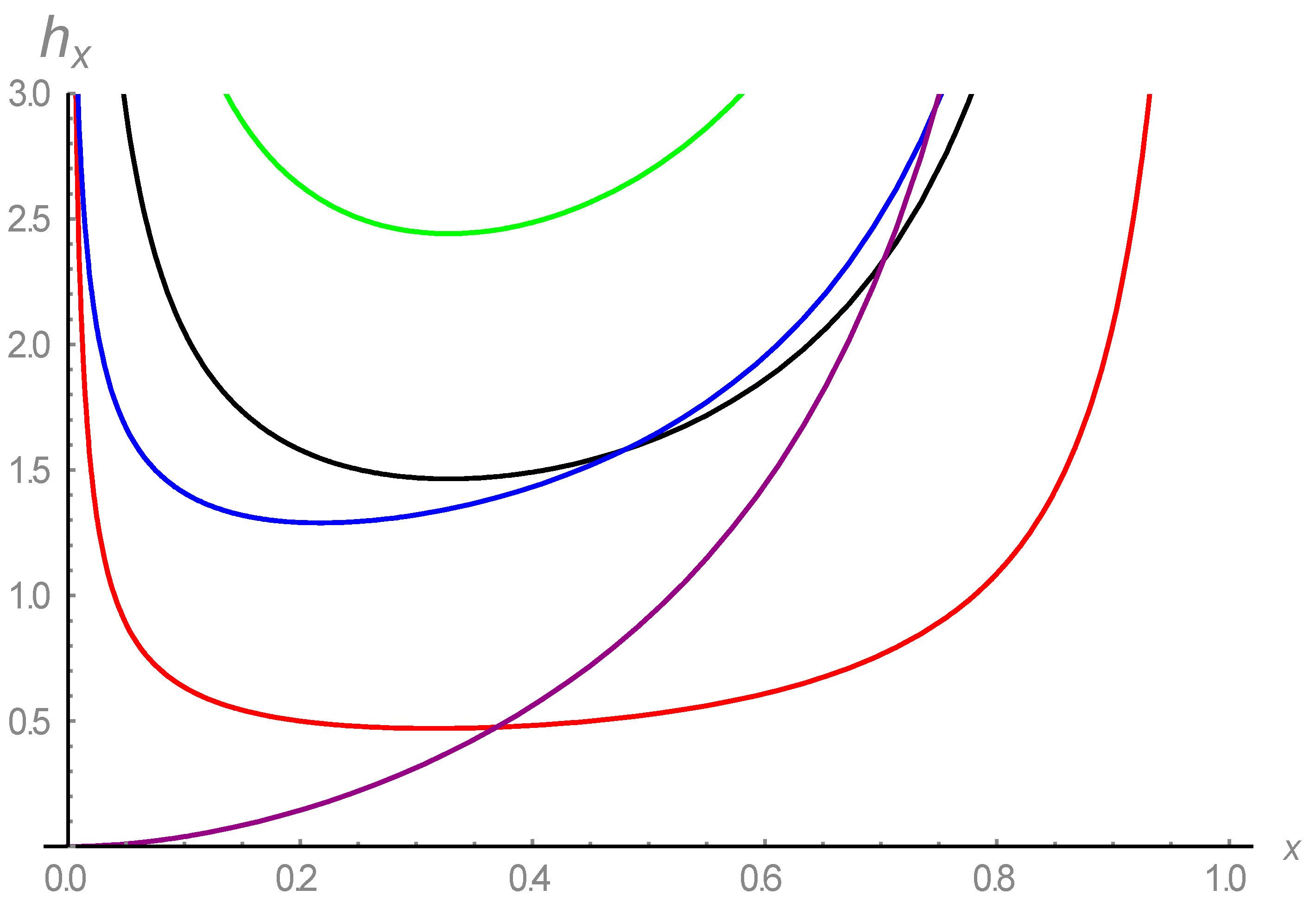
  • In addition, our model’s hazard rate assumes several forms, including U, increasing, and the bathtub shapes. Consequently, it may be beneficial to also study mortality and biological data;
  • The density function has increasing, decreasing, left-skewed, right-skewed, approximately symmetric, bathtub, and upside-down bathtub shapes, as shown in Figure 1. Our model’s advantageis thatit provides a wide range of shapes without requiring any additional parameters in its formulation;
  • This model is more adaptable to real data than beta (B), log-Lindley, power log-Lindley, power logarithmic (PL), reduced Kies (RK), log-gamma (LG), log-weighted power (LWP), transmuted power (TP), and Kumaraswamy (K) distributions, as will be shown in Section 7.
The remaining sections of the paper are structured as follows. In Section 2, we establish the three-parameter bounded beta (3PB) model and provide several probability density functions (PDF) and hazard rate function (HRF) plots. Section 3 covers the features of the 3PB distribution, including moments, conditional moments, mean residual life, mean deviations, Shannon entropy, and Rényi entropy. In Section 4, we derive the maximum likelihood estimations of the model parameters and confidence intervals by the Fisher information matrix. Section 5 provides the Bayes estimates of model parameters using the MCMC method. In Section 6, we compare the performance of these estimating approaches through a simulation study. In Section 7, we use two real-world applications to demonstrate the new model’s flexibility. Finally, in Section 8, we conclude the paper with some remarks.

2. The 3PB Distribution

This section introduces a new bounded model derived from the exponential transformation’s beta Sarhan–Zaindin modified Weibull (BSZMW) distribution, proposed by Saboor et al. [7]. Using the BSZMW distribution, whose PDF is defined by
f ( y ) = 1 B ( α , δ )   ( λ + γ k y k 1 ) ( 1 e λ y γ y k ) α 1 e δ λ y δ γ y k ;     y > 0 ,
where α , γ , λ , δ , k > 0 . Then, our distribution can be viewed as a result of BSZMW by setting k = 1 ,   λ + γ = β and employing the following transformation X = e Y .
Now, we define the cumulative distribution function (CDF) and PDF of our proposed model, which we refer to as the three-parameter bounded beta (3PB) distribution area, respectively, defined as
F ( x ) = x δ β δ B ( α , δ ) F 1 2 ( 1 α , δ ; 1 δ ; x β ) = B ( x β ; δ , α ) B ( α , δ ) ,
and
f ( x ) = β B ( α , δ ) x δ β 1 ( 1 x β ) α 1 ,   0 < x < 1 ,   α , δ , β > 0
where B ( x ; a , b ) = 0 x t a 1 ( 1 t ) b 1 d t is the incomplete beta function.
The survival function (SF) and HRF of the3PB model are, respectively, given as
S ( x )   = B ( x β ; δ , α ) B ( α , δ )
and
h ( x )   = β x δ β 1 ( 1 x β ) α 1 B ( α , δ ) B ( x β ; δ , α ) .
The 3PB distribution contains several distributions as special cases, as listed in Table 1.
Different plots of PDF of the 3PB model are displayed in Figure 1 for several parameter values, which showed that our proposed model PDF could be increasing, decreasing, left-skewed, right-skewed, approximately symmetric, bathtub, and upside-down bathtub shaped densities, and increasing, U, and bathtub shaped hazard rates as shown in Figure 2.

3. Mathematical Properties of the 3PB Model

This section presents some mathematical properties of the 3PB model, including moments, conditional moments, mean residual life, mean deviations, Shannon entropy, and Rényi entropy.

3.1. Moments

Theorem 1.
Let X be a random variable with 3PB density (3). Then the rth moment of X is
E [ X r ] = B ( α , δ + r / β ) B ( α , δ ) .
Proof. 
According to the definition of the r t h moment of X , we have
E [ X r ] = β B ( α , δ )   0 1   β B ( α , δ ) x δ   β   1 ( 1 x β ) α 1   d x .
Therefore, after some algebraic manipulations, we have the desired proof. □
Corollary 1.
The mean and variance of the 3PBmodel follows as
E [ X ] = B ( α , δ + 1 / β ) B ( α , δ ) ,
and
V a r [ X ] = B ( α , δ + 2 / β ) B ( α , δ ) ( E [ X ] ) 2 .
Proof. 
The proof follows by considering r = 1   and   r = 2   in Theorem 1. □

3.2. Conditional Moments

Predictive inference relies heavily on conditional moments.
Proposition 1.
The conditional moments E   [ X r | X > t ] of the 3PB model are obtained as
E   [ X r | X > t ] = 1 S ( t ) ( E ( X r ) β B ( α , δ ) t δ β + r ( δ β + r ) 2   F 1 2 ( 1 α , δ + r β ; 1 + δ + r β ; t β ) ) ,
where S ( t )   and   E [ X r ] are, respectively, defined by Equations (4) and (6), and F 1 2 ( a , b ; c ; z ) is thehypergeometric function defined as
F 1 2 ( a , b ; c ; z ) = m = 0 ( a ) m ( b ) m z m ( c ) m   m ! = 1 + a   b c z 1 ! + a ( a + 1 ) b ( b + 1 ) c ( c + 1 ) z 2 2 ! +
Proof. 
Using the following identity
E   [ X r | X > t ] = 1 S ( t ) ( E ( X r ) 0 t x r f ( x ) d x )
Using Equation (3), we have
0 t x r f ( x ) d x = β B ( α , δ )     t δ β + r ( δ β + r )     F 1 2 ( 1 α , δ + r β ;     1 + δ + r β ;     t β ) .
Applying the above result in Equation (8), we finish the proof. □

3.3. Mean Residual Life Function

The mean residual life (MRL) function represents the expected additional lifetime given that a component has survived until the time x .
Proposition 2.
The MRL function of the 3PB distribution is obtained as
Ω ( x ) = 1 S ( x ) { 1 x [ Γ ( δ ) Γ ( δ + 1 / β ) β B ( α , δ ) ( F ˜ 2 3 ( { 1 α , δ , δ + 1 / β } ; { 1 + δ , 1 + δ + 1 / β } ; 1 ) x δ β + 1 F ˜ 2 3 ( { 1 α , δ , δ + 1 / β } ; { 1 + δ , 1 + δ + 1 / β } ; x δ β ) ) ] } ,
where S ( x ) defined by Equation (4) and F ˜ q p ( a 1 , , a p ; b 1 , , b q ; z ) is the Regularized hypergeometric function defined as
F ˜ q p ( a 1 , , a p ; b 1 , , b q ; z ) = F q p ( a 1 , , a p ; b 1 , , b q ; z ) Γ ( b 1 ) Γ ( b q ) ,
where F q p ( a 1 , , a p ; b 1 , , b q ; z ) is the generalized hypergeometric function.
Proof. 
Using the following identity
Ω ( x ) = 1 S ( x ) x 1 [ 1 F ( t ) ] d t ,
Using Equation (2), we have
x 1 [ 1 F ( t ) ] d t = { 1 x [ Γ ( δ ) Γ ( δ + 1 / β ) β B ( α , δ ) ( F ˜ 2 3 ( { 1 α , δ , δ + 1 / β } ; { 1 + δ , 1 + δ + 1 / β } ; 1 ) x δ β + 1 F ˜ 2 3 ( { 1 α , δ , δ + 1 / β } ; { 1 + δ , 1 + δ + 1 / β } ; x δ β ) ) ] } .
Applying the above result in Equation (9), we finish the proof. □

3.4. Mean Deviations

The mean deviations are useful for measuring the amount of scattering in a population.
Proposition 3.
The mean deviations for the 3PB distribution are given by
δ = 2 μ F ( μ ) 2 B ( μ β ; δ + 1 / β , α ) B ( α , δ ) ,
where μ   and   F ( . ) are, respectively, defined by Equations (9) and (2).
Proof. 
Applying the following expression
δ = 2 μ   F ( μ ) 2 m ( μ ) ,
where
m ( z ) = 0 z x   f ( x ) d x = B ( z β ; δ + 1 / β , α ) B ( α , δ ) ,   z > 0 ,   z β 1 .
Applying the above result in Equation (10), we finish the proof. □

3.5. Entropy

Shannon entropy (Shannon [8]) and Rényi entropy (Rényi [9]) are two well-known ways of measuring entropy. Defined as
Ψ = E [ log ( f ( X ) ) ] ,
Λ = 1 1 γ   log [ R f   γ ( x ) d x ] ,       γ > 0       a n d     γ 1 ,
respectively. The two theorems that follow investigate exact forms of Shannon and Rényi entropies for the 3PB model and are as follows.
Theorem 2.
The Shannon entropy for the 3PB model is obtained as
Ψ = log ( B ( α , δ ) ) log ( β ) δ β 1 β ( ψ ( 0 ) ( δ ) ψ ( 0 ) ( α + δ ) )   ( α 1 ) ( ψ ( 0 ) ( α ) ψ ( 0 ) ( α + δ ) ) ,
where the Polygamma function of order m is defined by ψ ( m ) ( z ) = d m d z m ψ ( z ) , where ψ ( z ) is the digamma function and ψ ( 0 ) ( z ) = ψ ( z ) = Γ / ( z ) Γ ( z ) .
Proof. 
Using Equation (11), we have
Ψ = log ( B ( α , δ ) ) log ( β ) ( δ β 1 ) E     [ log ( X ) ] ( α 1 )   E [ log ( 1 X β ) ] .
The expression E     [ log ( x ) ] is immediate using Equation (3). Hence,
E     [ log ( x ) ] = ψ ( 0 ) ( δ ) ψ ( 0 ) ( α + δ ) β .
Also, the quantity E [ log ( 1 x β ) ] = ψ ( 0 ) ( α ) ψ ( 0 ) ( α + δ ) . Applying all the above results in Equation (11), we have the desired proof. □
Theorem 3.
TheRényi entropy for the 3PB distribution is
Λ = 1 1 γ     log ( β γ 1 ( B ( α , δ ) ) γ Γ [ 1 + γ ( α 1 ) ] Γ [ γ δ + 1 γ β ] Γ [ 1 + 1 β + γ ( α + δ 1 β 1 ) ] ) .
Proof. 
For our model
0 1 f γ ( x ) d x = ( β B ( α , δ ) ) γ 0 1   x γ ( δ β 1 ) ( 1 x β ) γ ( α 1 )   d x .
Then, the above expression reduces to
0 1 f γ ( x ) d x = β γ 1 ( B ( α , δ ) ) γ Γ [ 1 + γ ( α 1 ) ] Γ [ γ δ + 1 γ β ] Γ [ 1 + 1 β + γ ( α + δ 1 β 1 ) ] .
Using Equation (12), we have the desired proof. □

4. Classical Estimations

This section evaluates the MLEs and confidence intervals based on the approximate Fisher information matrix of the unknown parameters α ,   β ,     and   δ .

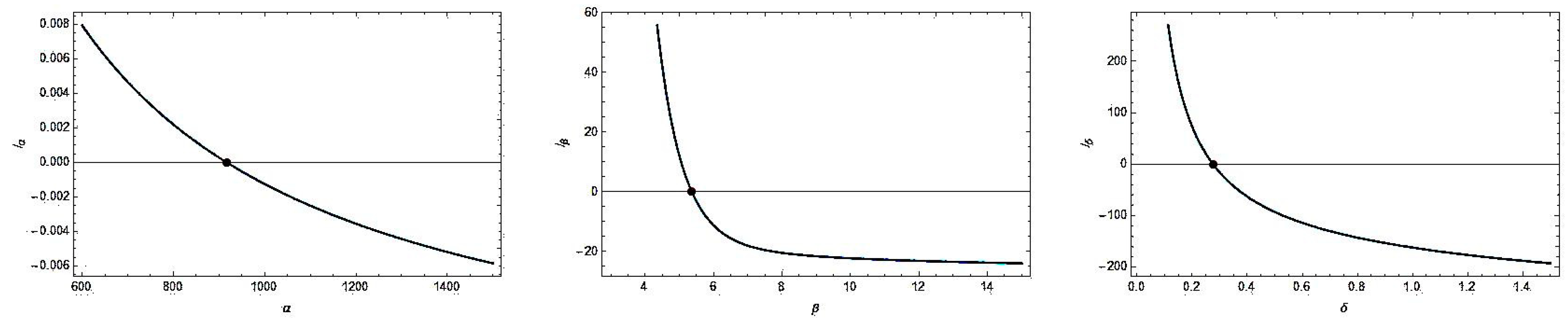
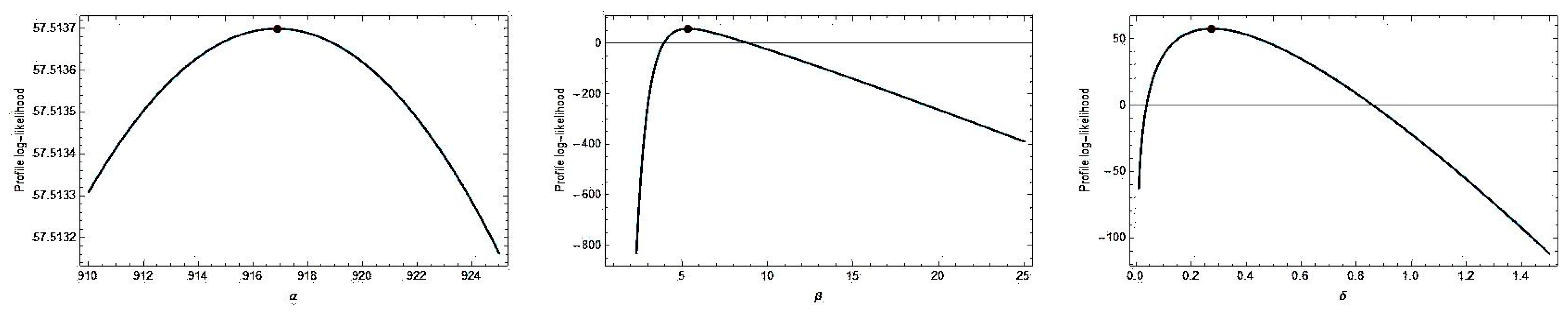
4.1. Maximum Likelihood Estimation

Let X 1 , X 2 , , X n be a random sample from 3PB distribution, and then the likelihood function is given by
L ( α , δ , β ; x ) = ( β B ( α , δ ) ) n i = 1 n x i δ β 1 i = 1 n [ 1 x i β ] α 1 .
The log-likelihood function ( α , δ , β ) is given by
( α , δ , β ; x ) = n ln β n ln B ( α , δ ) ( δ β 1 ) i = 1 n ln x i + ( α 1 ) i = 1 n ln ( 1 x i β )
Then, we can have
α = n ( ψ ( 0 ) ( α ) ψ ( 0 ) ( α + δ ) ) + i = 1 n ln [ 1 x i β ] ,
β = n β δ i = 1 n ln [ x i ] + ( α 1 ) i = 1 n x i β ln [ x i ] 1 x i β ,
δ = n ( ψ ( 0 ) ( δ ) ψ ( 0 ) ( α + δ ) ) β i = 1 n ln [ x i ] ,
Let α = 0 ,   β = 0 ,   and   δ = 0 , then we can use the Newton–Raphson method to solve nonlinear equations and find the unknown parameters.

4.2. Asymptotic Confidence Intervals

Now, to find the approximate confidence intervals for the parameters α ,   β ,     and   δ ,we can use the following asymptotic distribution of the MLEs
[ ( α ^ α ) ,   ( β ^ β ) , (   δ ^ δ )   ] N ( 0 , I 1 ( α ,   β , δ ) )
where I 1 ( α ,   β , δ ) is the variance–covariance matrix of the parameters α ,   β ,     and   δ , and it can be approximated by the inverse of the observed Fisher-information matrix. The observed Fisher-information matrix is given by
I ( α ^ ,   β ^ , δ ^ ) = ( 2 α 2 2 α β 2 α δ 2 β α 2 β 2 2 β δ 2 δ α 2 δ β 2 δ 2 ) ( α , β , δ   ) = ( α ^ ,   β ^ , δ ^ ) ,
where
2 α 2 = n ( ψ ( 1 ) ( α ) ψ ( 1 ) ( α + δ ) ) ,
2 α β = i = 1 n x i β ln [ x i ] 1 x i β ,
2 β 2 = n β 2 + ( α 1 ) i = 1 n { x i 2 β ln [ x i 2 ] ( 1 x i β ) 2 x i β ln [ x i 2 ] 1 x i β } ,
2 α δ = n ( ψ ( 1 ) ( α + δ ) ) ,
2 δ β = i = 1 n ln [ x i ] ,
2 δ 2 = n ( ψ ( 1 ) ( δ ) ψ ( 1 ) ( α + δ ) ) .
Then, the approximate 100 ( 1 γ ) % two-sided confidence intervals for α ,   β ,   and   δ are, respectively, given by
[ α ^ M L ± Z γ / 2 I 11 1 ( α ^ M L ) ,   ( β ^ M L ± Z γ / 2 I 22 1 ( β ^ M L ) , ( δ ^ M L ± Z γ / 2 I 33 1 ( δ ^ M L )     ]
where Z γ / 2 is the upper 100 ( γ / 2 ) t h percentile of the standard normal distribution.

5. Bayesian Estimation
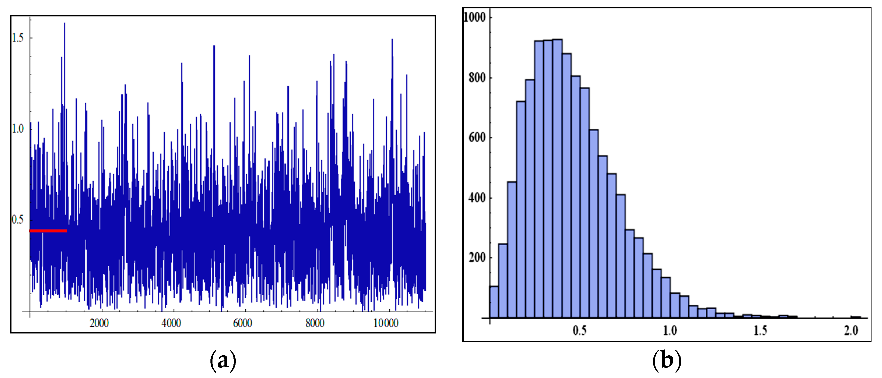
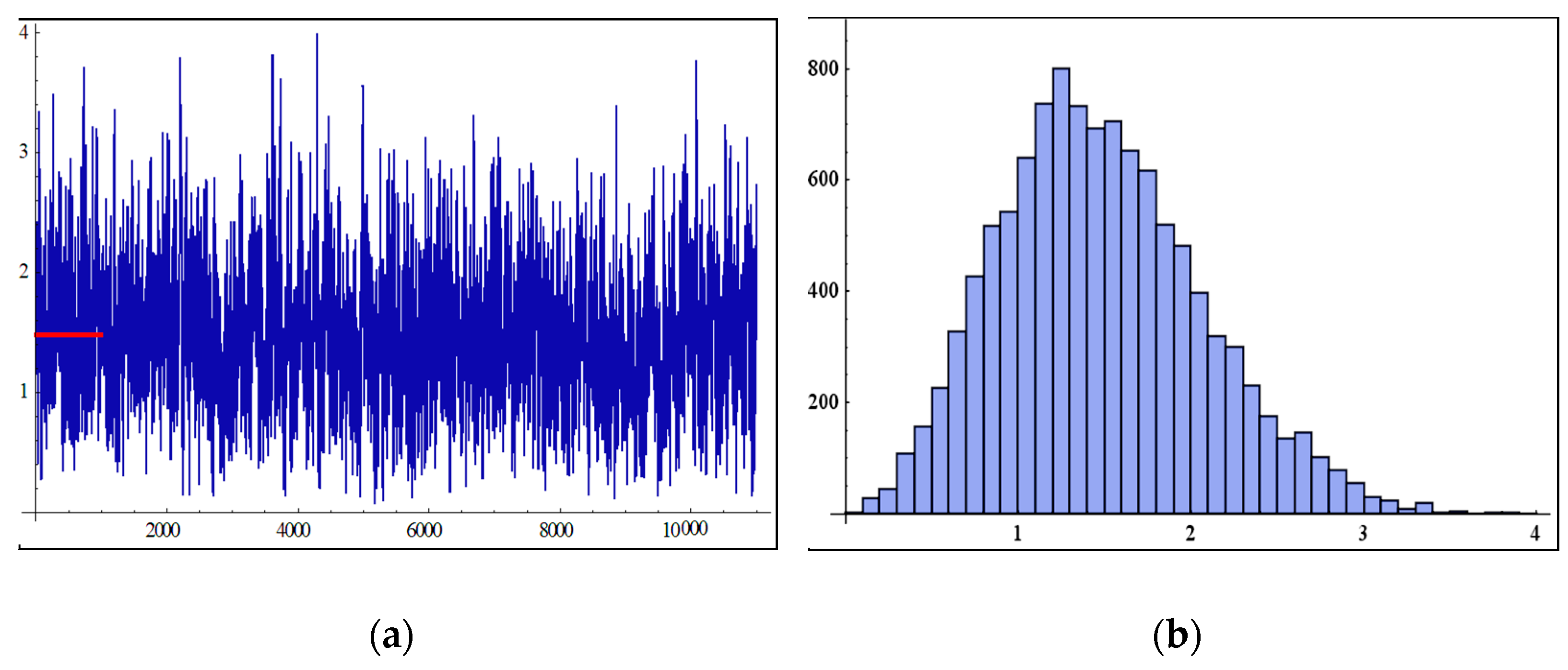
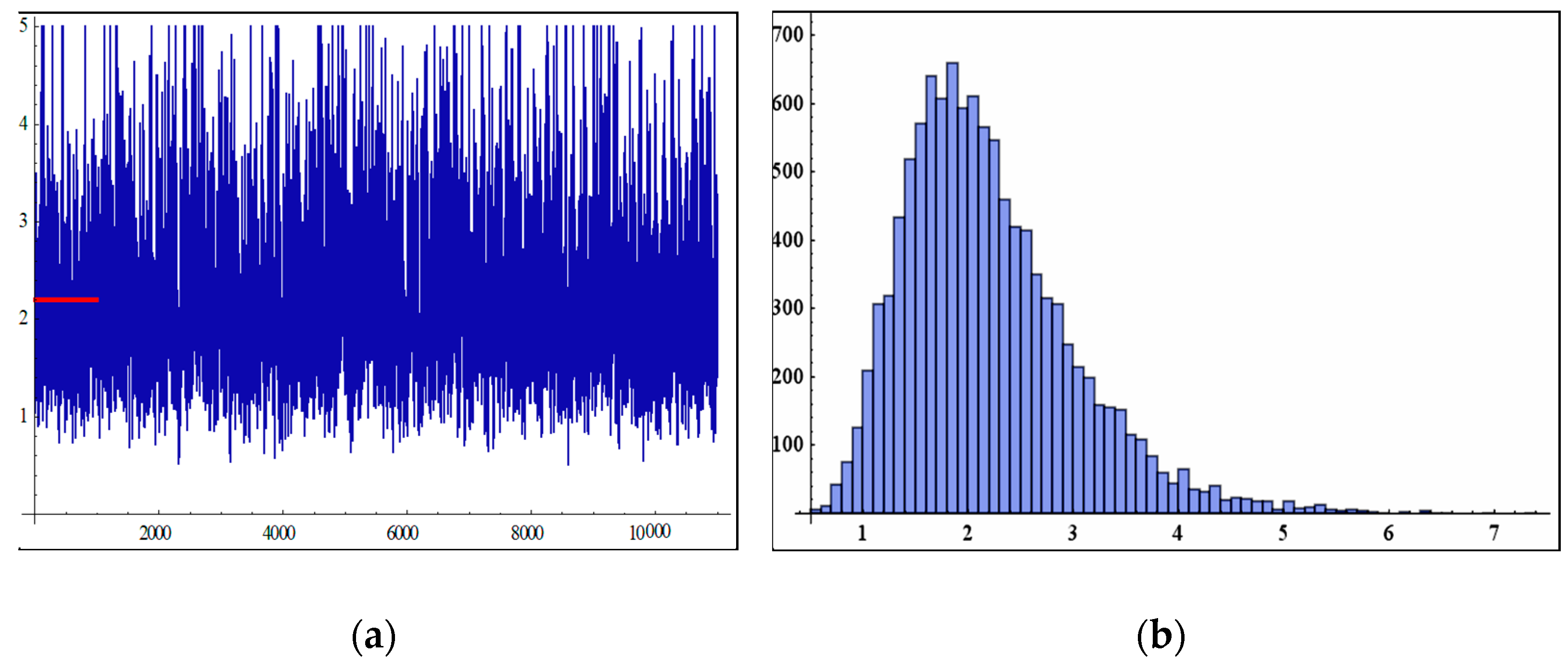
This section presents the Bayes estimates (BEs) of the parameters α ,   β ,     and   δ under SE and LINEX loss function by using informative priors.
Suppose that the parameters α ,   β ,     and   δ are independent, as
π 1 ( α ) α a 1 1 e α / b 1 ,                   a 1 , b 1 > 0
π 2 ( β ) β a 2 1 e β / b 2 ,                   a 2 , b 2 > 0
π 3 ( δ ) δ a 3 1 e δ / b 3 ,                     a 3 , b 3 > 0
.
For more details for using the gamma prior, see Kim et al. [10] and Singh et al. [11].
Then, the joint prior is given by
π ( α , δ , β ) α a 1 1 β a 2 1 δ a 3 1 e α / b 1 β / b 2 δ / b 3 ,       a 1 ,     a 2 ,     a 3 ,     b 1 ,     b 2 ,     b 3 > 0
From Equations (13) and (14), the joint posterior density function is
π * ( α , β , δ | x ) L ( α , β , δ ; x ) π ( α , β , δ )
  α a 1 1 β a 2 1 δ a 3 1 e α / b 1 β / b 2 δ / b 3     ( β B ( α , δ ) ) n i = 1 n x i δ β 1 i = 1 n [ 1 x i β ] α 1
Then, the Bes of the function Φ ( α , β , δ ) under SE loss and LINEX loss functions, can be written, respectively, as
Φ ^ S E ( α , β , δ ) = E [ Φ ( α , β , δ ) | x ] = 0 0 0 Φ ( α , β , δ ) π ( α , β , δ | x ) d α d β d δ = 0 0 0 Φ ( α , β , δ ) α a 1 1 β a 2 1 δ a 3 1 e α / b 1 β / b 2 δ / b 3     ( β B ( α , δ ) ) n i = 1 n x i δ β 1 i = 1 n [ 1 x i β ] α 1 d α d β d δ
Φ ^ L I N E X ( α , β , δ ) = 1 c ln [ 0 0 0 e c Φ ( α , β , δ ) π ( α , β , δ | x ) d α d β d δ ] = 1 c ln   [ 0 0 0 e c Φ ( α , β , δ ) α a 1 1 β a 2 1 δ a 3 1 e α / b 1 β / b 2 δ / b 3     ( β B ( α , δ ) ) n × i = 1 n x i δ β 1 i = 1 n [ 1 x i β ] α 1 d α d β d δ ] ,
where c is an arbitrary constant.

MCMC Method

We will present the MCMC method to find the BEs and CI based on the SE and LINEX loss functions;so from Equation (15) we can write the conditional posterior density functions of the model parameters α ,   β ,     and   δ , as follows
π α ( α | β , δ ; x ) α a 1 1 e α / b 1     ( α + δ α ) n i = 1 n [ 1 x i β ] α 1
π β ( β | α , δ ; x ) β n + a 2 1 e β / b 2   i = 1 n x i δ β i = 1 n [ 1 x i β ] α 1 ,
π δ ( δ | α , β ; x ) δ a 3 1 e δ / b 3     ( α + δ δ ) n i = 1 n x i δ β .
The Equations (18)–(20) cannot be reduced analytically to known distributions from the conditional posterior distributions of α ,   β ,   and   δ . So, to solve this problem, we use the Metropolis–Hastings algorithm which reduces the correlation between the generated variables. These are the advantages of the Metropolis–Hastings algorithm; see Upadhyay and Gupta [12]. So, we used the following algorithm.

6. Simulation Study

This section chose different sample sizes to present the simulation study using the Algorithm 1.
Algorithm 1
  • Begin with an ( α ( 0 ) = α ^ M L E   ,     β ( 0 ) = β ^ M L E ,       and     δ ( 0 ) = δ ^ M L E ) .
  • Set t = 1.
  • Use MH algorithm to generate α(t) from π α ( α ( t 1 ) | β ( t 1 ) , δ ( t 1 ) ; x ) , generate β(t) from π β ( β ( t 1 ) | α ( t ) , δ ( t 1 ) ; x ) , and generate δ(t) π δ ( δ ( t 1 ) | α ( t ) , β ( t ) ; x ) .
  • Set t = t + 1
  • Repeat steps 2–4 N times.
  • Obtain α ( t )   ,   β ( t ) and     δ ( t )   , t = M + 1 ,   ,   N ,   then ,   the   approximate   means   of   Φ ( α , δ , β )   and   exp [     c     Φ ( α , β , δ ) ]   are   given ,   respectively ,   by
    E [ Φ ( α , β , δ ) | x ] = 1 N M = M + 1 N Φ ( α ( t ) , β ( t ) ,   δ ( t ) )
    E [ exp ( c Φ ( α , β , δ ) | x ) ] = 1 N M t = M + 1 N exp [ c Φ ( α ( t ) , β ( t ) , δ ( t ) ) | x ] ,
    where M is the burn-in period.
    Then ,   the   point   estimation   of   Φ ( α , β , δ ) under   S E   and   L I N E X   loss   functions   by   MCMC   method   are   given ,   by
    Φ ^ S E ( α , β , δ ) = E [ Φ ( α , β , δ ) | x ]
    Φ ^ L I N E X ( α , β , δ ) = 1 c ln [ E ( exp ( c Φ ( α , β , δ ) | x ) ]
  • Repeat 1–6H time and arrange the values of the estimated parameters as α ^ S E [ 1 ] ,   ,   α ^ S E [ H ] , β ^ S E [ 1 ] ,   ,   β ^ S E [ H ] ,   and     δ ^ S E [ 1 ] ,   ,   δ ^ S E [ H ] . Then, the 100 (1 − γ)% credible intervals for α ,   β ,     and   δ are   ( α ^ S E [ γ 2 ) H ] ,   α ^ S E [ ( 1 γ 2 ) H ] )   ( β ^ S E [ γ 2 ) H ] ,   β ^ S E [ ( 1 γ 2 ) H ] ) ,   and     ( δ ^ S E [ γ 2 ) H ] ,   δ ^ S E [ ( 1 γ 2 ) H ] ) ,   respectively .
Plots in Figure 3a, Figure 4a and Figure 5a show the trace plots of 10,000 MCMC samples for the posterior distribution of α ,   β   and   δ , and plots in Figure 3b, Figure 4b and Figure 5b display the histogram plots of generated α ,   β   and   δ , when n = 50.
We can notice from the simulation study, that:
  • In Table 2, when the sample size increases, the MSEs of MLEs and BEs decrease as the sample size increases, except for a few cases. This may be due to fluctuations in data.
  • The BEs give more accurate results through the MSEs than the MLEs for all sample size n.
  • The MSEs under LINEX loss function ( c = 1 ) have the smallest as compared with estimates under MLEs and SE loss function.
  • It was also observed for very large sample sizes that the BEs and the MLEs become closer in terms of MSEs. That is, for very large sample sizes, the performances are so far similar as expected.
  • In Table 3, the length of credible Cis α ,   β ,   and   δ decreases as the sample size increases and the credible CIs give more accurate results than MLE CIs through the length and the CPs of CIs.
  • It can be easily checked that the values of CPs are quite close to the nominal level 0.95 in many of the considered cases of credible CIs.

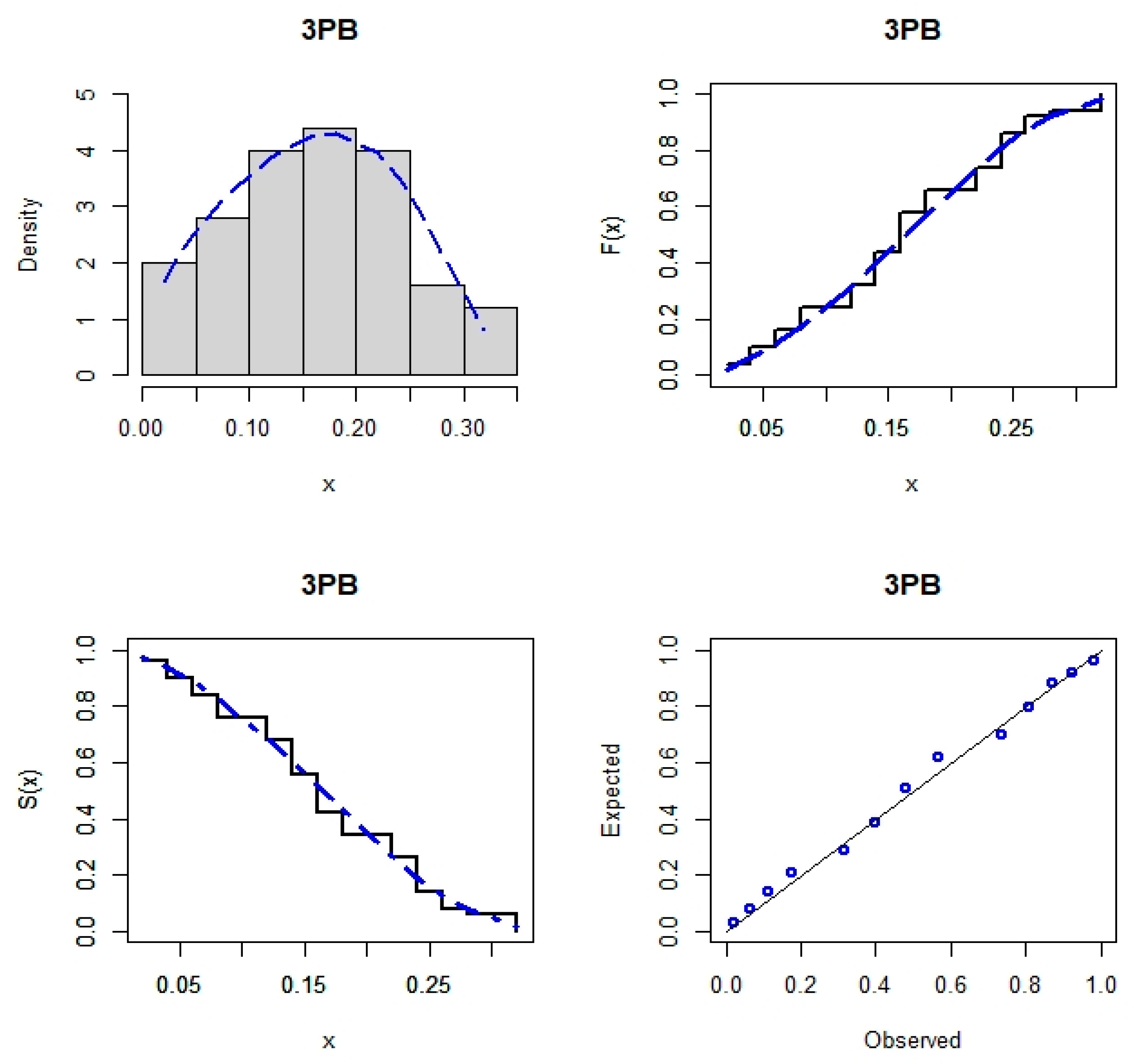
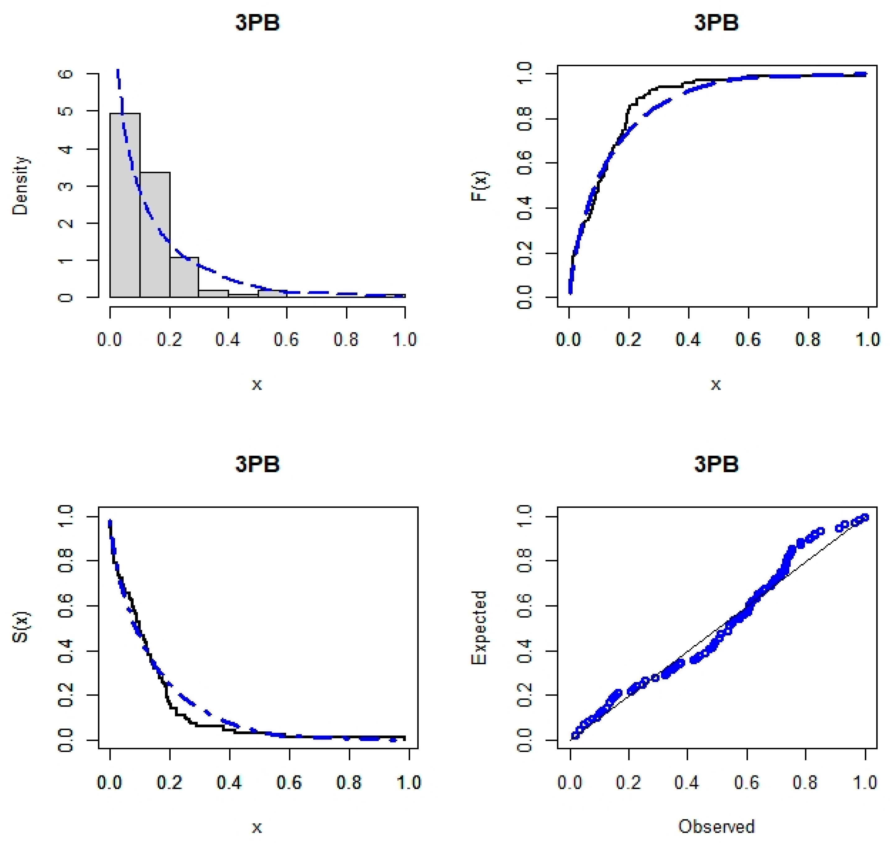
7. Real Data Analysis

In this section, we consider two real data sets to illustrate the flexibility of the proposed distribution. In the first real data set of 50 observations on burr (in the millimeter unit), the hole diameter is 12 mm, and the sheet thickness is 3.15 mm. It was introduced by Dasgupta [13]. The second real data set represents the stress-rupture life of Kevlar 49/epoxy strands subjected to constant sustained pressure at the 90% stress level until all had failed. The failure times are expressed in hours. This was introduced by Barlow et al. [14]. We perform a “unit range” operation on the second real data set by dividing them by 7.99.
The 3PB distribution is compared with other distributions, such as beta (B), log-Lindley (LL) [15], power log-Lindley (PLL) [16], power logarithmic (PL) [17], reduced Kies (RK) [18], log-gamma (LG) [19], log-weighted power (LWP) [20], transmuted power (TP) [20], and Kumaraswamy (K) distributions.
The competing models were compared using some analytical measures, including some information criteria (IC), such as Akaike IC (AIC), corrected AIC (CAIC), and Hannan–Quinn IC (HQIC), along with some goodness-of-fit measures, such as Anderson–Darling (AD), Cramer–von Mises (CM), and Kolmogorov–Smirnov (KS) with its p-value (KS p-value) to determine the best-fitting model for the considered real data sets.
Wolfram Mathematica version 12.0 was used to calculate analytical measurements and MLE with their standard errors (SEs) for all compared models which are presented in Table 4 and Table 5 for burr and stress-rupture data sets, respectively. We conclude that the 3PB distribution fits the analytical data sets better than competing models.
Figure 6 and Figure 7 show the estimated PDF, CDF, and SF of 3PD distribution with P-P plots for burr and stress-rupture data sets, respectively. Figure 8 and Figure 9 illustrate, burr and stress-rupture data sets, respectively, the existence and uniqueness of estimated parameters of 3PB model. Figure 10 and Figure 11 show the behavior of the estimated log-likelihood function for burr and stress-rupture data sets, respectively.

8. Conclusions

This article presents a new three-parameter distribution for modeling bounded data. The new model, called the three-parameter bounded beta (3PB) distribution, is derived from the beta Sarhan–Zaindin modified Weibull (BAZMW) distribution by the exponential transformation. Its mathematical features are derived, including moments, conditional moments, mean residual life, mean deviations, Shannon entropy, and Rényi entropy. Maximum likelihood estimations of the model parameters and confidence intervals by Fisher information matrix are derived. Bayes estimates of model parameters using the MCMC method are provided. A simulation study to compare all proposed estimation methods is presented. Two applications demonstrate that 3PB distribution is superior to other competing models in terms of fit. As a future work, the proposed distribution might be utilized for modeling and analyzing data in fields such as reliability engineering, medicine, economics, survival analysis, and life testing. The suggested distribution may also be explored as a bivariate extension, and this would, presumably, bea discrete case. Also, we can use regression analysis for our proposed model. Finally, the problem of MLEs and BSs for the partially accelerated life test model under the Type-II hybrid censoring scheme of 3PB distribution can be extended to include informative priors and also to consider other techniques, such as the Markov Chain Monte Carlo (MCMC) technique to compute the approximate Bayes estimates under loss functions, to investigate their performances, and to compare them with those of the MLEs.

Author Contributions

Formal analysis, A.M.T.A.E.-B.; Resources, F.A.A.; Investigation, M.A.F.; Software, A.M.G. All authors have read and agreed to the published version of the manuscript.

Funding

This research received no external funding.

Data Availability Statement

Datasets are available in real data analysis section.

Conflicts of Interest

The authors declare no conflict of interest.

References

  1. Johnson, N.L.; Kemp, A.W.; Balakrishnan, N. Continuous Univariate Distributions, 2nd ed.; Wiley: New York, NY, USA, 1995; Volume 1. [Google Scholar]
  2. Johnson, N.L.; Kotz, S.; Balakrisnan, N. Continuous Univariate Distributions, 2nd ed.; Wiley: New York, NY, USA, 1994; Volume 1. [Google Scholar]
  3. Chotikapanich, D.; Rao, D.S.P.; Tang, K.K. Estimating income inequality in China using grouped data and the generalized beta distribution. In Review of Income and Wealth; Wiley: Hoboken, NY, USA, 2007; Volume 53, pp. 127–147. ISSN 1475-4991. [Google Scholar]
  4. Ng, D.W.W.; Koh, S.K.; Sim, S.Z.; Lee, M.C. The study of properties in generalized beta distribution. IOP Conf. Series J. Phys. 2019. [Google Scholar] [CrossRef]
  5. Albassam, M.; Soliman, E.E.A.; Ali, S.S. Bayesian Estimation of Multivariate Pure Moving Average Processes. IEEE Access 2022, 10, 14225–14235. [Google Scholar] [CrossRef]
  6. Bertschinger, N.; Mozzhorin, I. Bayesian estimation and likelihood-based comparison of agent based volatility models. J. Econ. Interact. Coord. 2021, 16, 173–210. [Google Scholar] [CrossRef]
  7. Saboor, A.; Bakouch, H.S.; Khan, M.N. Beta Sarhan-Zaindin modified Weibull distribution. Appl. Math. Model. 2016, 40, 6604–6621. [Google Scholar] [CrossRef]
  8. Shannon, C.E. Prediction and entropy of printed English. Bell Syst. Tech. J. 1951, 30, 50–64. [Google Scholar] [CrossRef]
  9. Rényi, A. On measures of entropy and information. In Contributions to the Theory of Statistics, Proceedings of the Fourth Berkeley Symposium on Mathematical Statistics and Probability, Berkeley, CA, USA, 20 June–30 July 1960; University of California Press: Berkeley, CA, USA, 1961; Volume 1, pp. 547–561. [Google Scholar]
  10. Kim, C.; Jung, J.; Chung, Y. Bayesian estimation for the generalized Weibull model under Type II progressive censoring. Stat. Pap. 2011, 52, 53–70. [Google Scholar] [CrossRef]
  11. Singh, S.K.; Singh, U.; Kumar, M.; Vishwakarma, P.K. Classical and Bayesian inference for an extension of the exponential distribution under progressive Type- II censored data with binomial removals. J. Stat. Appl. Prob. Lett. 2014, 1, 75–86. [Google Scholar] [CrossRef]
  12. Upadhyay, S.K.; Gupta, A. Bayes analysis of modified Weibull distribution via Markov chain Monte Carlo simulation. J. Stat. Compu. Simul. 2010, 80, 241–254. [Google Scholar] [CrossRef]
  13. Dasgupta, R. On the distribution of burr with applications. Sankhya B 2011, 73, 1–19. [Google Scholar] [CrossRef]
  14. Barlow, R.; Toland, R.; Freeman, T. A Bayesian analysis of stress-rupture life of kevlar/epoxy spherical pressure vessels. In Accelerated Life Testing and Experts Opinions in Reliability; Clarotti, C., Lindley, D., Eds.; Elsevier Science Ltd.: Amsterdam, The Netherlands, 1988; pp. 203–236. [Google Scholar]
  15. Gómez-Déniz, E.; Sordo, M.A.; Calderín-Ojedac, E. The log-Lindley distribution as an alternative to the beta regression model with applications in insurance. Insur. Math. Econ. 2014, 54, 49–57. [Google Scholar] [CrossRef]
  16. Abd El-Bar, A.M.T.; Da Silva, W.B.F.; Nascimento, A.D.C. An extended log-Lindley-G family: Properties and experiments in repairable data. Mathematics 2021, 9, 3108. [Google Scholar] [CrossRef]
  17. Abd El-Bar, A.M.T.; Lima, M.S.; Ahsanullah, M. Some inferences based on a mixture of power function and continuous logarithmic distribution. J. Taibah Univ. Sci. 2020, 14, 1116–1126. [Google Scholar] [CrossRef]
  18. Kumar, C.S.; Dharmaja, S.H.S. On reduced Kies distribution. In Collection of Recent Statistical Methods and Applications; Department of Statistics, University of Kerala Publishers: Trivandrum, India, 2013; pp. 111–123. [Google Scholar]
  19. Amini, M.; Mir Mostafaee, S.M.T.K.; Ahmadi, J. Log-gamma-generated families of distributions. Statistics 2014, 48, 913–932. [Google Scholar] [CrossRef]
  20. Chesneau, C. On a logarithmic weighted power distribution: Theory, modeling and applications. J. Math. Sci. Adv. Appl. 2021, 67, 1–59. [Google Scholar] [CrossRef]
Figure 1. Plots of 3PBPDFs: (a) α = β = 1, δ = 1.3 (red), α = 1, β = 0.2, δ = 1.3 (green), α = 1, β = 2.2, δ = 1.3 (black), α = 3, β = 1.9, δ = 1.4 (purple), α = 4, β = 1.2, δ = 1.3 (black). (b) α = 0.6, β = 0.2, δ = 1 (blue), α = 0.6, β = 0.5, δ = 1 (red), α = 0.7, β = 0.6, δ = 1 (purple), α = 1, β = 0.8, δ = 1.2 (black), α = 1, β = 0.9, δ = 1.3 (green).
Axioms 11 00504 g001
Figure 2. Plots of 3PB HRF: α = 0.2, β = 0.1, δ = 2 (red), α = 0.6, β = 0.2, δ = 1 (black), α = 0.7, β = 0.9, δ = 1 (blue), α = 1, β = 2.2, δ = 1.3 (purple), α = 1, β = 0.2, δ = 1 (green).
Axioms 11 00504 g002
Figure 3. (a) Simulation number of α obtained by MCMC method. (b) Histogram of α obtained by MCMC method.
Axioms 11 00504 g003
Figure 4. (a) Simulation number of β obtained by MCMC method. (b) Histogram of β obtained by MCMC method.
Axioms 11 00504 g004
Figure 5. (a) Simulation number of δ obtained by MCMC method. (b) Histogram of δ obtained by MCMC method.
Axioms 11 00504 g005
Figure 6. Histogram of burr data with the estimated PDF, CDF, and SF of 3PB model with its P-P plots.
Axioms 11 00504 g006
Figure 7. Histogram of stress-rupture data with the estimated PDF, CDF, and SF of 3PB model with its P-P plots.
Axioms 11 00504 g007
Figure 8. Existence and uniqueness plots for 3PB model parameters for burr data set.
Axioms 11 00504 g008
Figure 9. Existence and uniqueness plots for 3PB model parameters for stress-rupture data set.
Axioms 11 00504 g009
Figure 10. Behavior of log-likelihood function with 3PB model parameters for burr data set.
Axioms 11 00504 g010
Figure 11. Behavior of log-likelihood function with 3PB model parameters for the stress-rupture data set.
Axioms 11 00504 g011
Table 1. Special cases of the 3PB.
Parametric Values and Transformation in (3)Models
β = 1 Beta distribution
β = 1     and   α = δ = 1 / 2 Arcsine distribution
x = e y and   β = 0 Beta exponential distribution
x = e y ,   β = 0 ,     and   α = δ = 1 Exponential distribution
x = e y ,   β = 0   and   δ = 1 Exponentiated exponential distribution
β = α = δ = 1 Uniform distribution on (0, 1)
δ = 1   Kumaraswamy distribution
x = y / b   , b > 0   Generalized beta of the first kind model
β = 0   and   α = γ + 1 Beta power distribution
Table 2. MLE, BE and with their *MSEs for the parameters ( α = 0.5 ,   β = 1.5 ,   δ = 2 ) and values of the prior a 1 = 0.58 ,       b 1 = 0.93 ,       a 2 = 0.28 ,       b 2 = 0.66 and a 3 = 0.35 ,       b 3 = 0.25 .
n MLEBE
SELINEXc = 1
10 α
β
δ
0.247 (1.832)0.373 (0.942)0.391 (0.744)
1.214 (0.641)1.291 (0.321)1.332 (0.266)
2.784 (0.814)2.541 (0.342)2.322 (0.388)
20 α
β
δ
0.251 (1.511)0.392 (0.795)0.399 (0.553)
1.143 (0.622)1.313 (0.314)1.343 (0.392)
2.527 (0.702)2.392 (0.284)2.321 (0.251)
30 α
β
δ
0.291 (1.421)0.412 (0.484)0.432 (0.439)
1.209 (0.497)1.365 (0.278)1.382 (0.331)
2,563 (0.773)2.313 (0.279)2.275 (0.215)
40 α
β
δ
0.301 (1.252)0.431 (0.421)0.439 (0.462)
1.292 (0.447)1.397 (0.185)1.413 (0.158)
2.413 (0.559)2.293 (0.212)2.311 (0.198)
50 α
β
δ
0.347 (0.873)0.441 (0.218)0.452 (0.195)
1.256 (0.119)1.429 (0.094)1.463 (0.084)
2.392 (0.235)2.143 (0.182)2.114 (0.089)
* MSEs are given in bracket.
Table 3. Lengths and coverage probabilities (CPs) of 95% CIs of the parameters ( α = 0.5 ,     β = 1.5 ,   δ = 2 ) and values of the prior a 1 = 0.58 ,       b 1 = 0.93 ,       a 2 = 0.28 ,     b 2 = 0.66 , and a 3 = 0.35 ,     b 3 = 0.25 .
n MLEBE
LengthCPLengthCP
10α
β
δ
1.4370.7930.5430.864
4.5420.7721.3940.852
2.4820.9020.9340.934
20α
β
δ
1.3740.8320.5740.877
4.3260.8291.4850.869
2.1650.9210.8540.994
30α
β
δ
1.3940.8050.3950.896
3.9250.7931.2930.875
1.9470.9110.7951
40α
β
δ
1.2430.8490.3210.918
4.1860.8361.1470.878
2.0950.9320.7530.957
50α
β
δ
0.9830.8730.2010.929
3.7440.8841.0820.914
1.7820.9390.5930.971
Table 4. Numerical information criteria values with the goodness-of-fit measures for the burr data set.
Model−LAICCAICHQICADCMKSKS
p-Value
Est. Parameters (SEs)
3PB−57.513−109.027−108.506−106.8430.434050.073040.099880.70076 α = 916.89 (2899.91)
β = 5.36001 (2.91255)
δ = 0.275398 (0.188897)
B−54.606−105.213−104.958−103.7570.912340.153900.141460.26969a = 2.68257 (0.507179)
b = 13.8658 (2.82802)
LL−31.826−59.653−59.3977−58.19686.567591.226770.318130.00008 β = 1.00664 (0.0762406)
λ = 0.00001 (0.129734)
PLL−31.826−57.653−57.1313−55.46876.567591.226770.318130.00008 α = 1.89694 (0.645369)
σ = 0.530664 (0.151324)
λ = 1.03 × 10 13 (1.23461 × 10 7 )
PL−31.8265−57.653−57.1313−55.46876.56761.226770.318130.00008 α = 0.006640 (0.100664)
β = 0.003714 (27.6384)
δ = 2.3294 × 10 6 (792681)
RK−11.6763−21.3526−21.2692−20.624421.71944.865160.56334<0.0001a = 0.736768 (0.087676)
LG−31.8265−61.653−61.5697−60.92496.567591.226770.318130.00008σ = 1.00664 (0.100664)
LWP−31.8265−59.653−59.3977−58.19686.567591.226770.318130.00008 α = 1.00664 (0.173704)
λ = 1.0 (0.511507)
TP−30.3176−56.6353−56.3799−55.1796.798421.264380.320940.00006 α = 0.733619 (0.11218)
λ = 1.0 (0.631411)
K−56.0687−108.137−107.882−106.6810.677630.104210.110250.57766a = 2.0774 (0.25485)
b = 33.1374 (13.9216)
Table 5. Numerical information criteria values with the goodness-of-fit measures for the stress-rupture data set.
Model−LAICCAICHQICADCMKSKS
p-Value
Est. Parameters (SEs)
3PB−100.494−194.989−194.741−191.8131.413920.219180.107070.19717 α = 3.16676 (0.424279)
β = 0.00849 (0.204003)
δ = 135.631 (3282.79)
B−97.5517−191.103−190.981−188.9861.730530.253680.129560.06733a = 0.66105 (0.079057)
b = 3.84874 (0.607836)
LL−95.7616−187.523−187.401−185.4064.084760.681730.191140.00124 β = 0.72667 (0.052133)
λ = 0.025905 (0.03995)
PLL−95.7616−185.523−185.276−182.3474.084760.681730.191140.00124α = 1.42502 (2995.65)
σ = 0.50994 (1071.99)
λ = 0.036915 (77.6033)
PL−84.6077−163.215−162.968−160.03918.06043.661770.33304<0.0001 α = 4.88982 (0.070983)
β = 0.00148 (0.238805)
δ = 0.248041 (3.97841)
RK−52.5838−103.168−103.127−102.10928.67856.410160.459060.0000a = 0.45559 (0.035412)
LG−95.3337−188.667−188.627−187.6093.941750.653390.188050.00157 σ = 0.73344 (0.051605)
LWP−95.7616−187.523−187.401−185.4064.084760.681730.191140.00124 α = 0.72667 (0.052133)
λ = 0.98152 (0.027749)
TP−93.9055−183.811−183.689−181.6944.549640.760990.198440.00070 α = 0.53593 (0.0402053)
λ = 0.97495 (0.038706)
K−98.9507−193.901−193.779−191.7841.558110.2316370.117670.121948a = 0.70876 (0.068023)
b = 3.45759 (0.554958)
Publisher’s Note: MDPI stays neutral with regard to jurisdictional claims in published maps and institutional affiliations.

