Article

Statistical Analysis of Alpha Power Exponential Parameters Using Progressive First-Failure Censoring with Applications

1
Department of Statistics, Faculty of Science, King Abdulaziz University, Jeddah 21589, Saudi Arabia
2
Department of Statistics, Faculty of Commerce, Zagazig University, Zagazig 44519, Egypt
3
Department of Mathematical Sciences, College of Science, Princess Nourah bint Abdulrahman University, P.O. Box 84428, Riyadh 11671, Saudi Arabia
4
Faculty of Technology and Development, Zagazig University, Zagazig 44519, Egypt
*
Author to whom correspondence should be addressed.
Axioms 2022, 11(10), 553; https://doi.org/10.3390/axioms11100553
Submission received: 22 August 2022 / Revised: 26 September 2022 / Accepted: 3 October 2022 / Published: 13 October 2022
(This article belongs to the Special Issue Computational Statistics & Data Analysis)

Abstract

:
This paper is an endeavor to investigate some estimation problems of the unknown parameters and some reliability measures of the alpha power exponential distribution in the presence of progressive first-failure censored data. In this regard, the classical and Bayesian approaches are considered to acquire the point and interval estimates of the different quantities. The maximum likelihood approach is proposed to obtain the estimates of the unknown parameters, reliability, and hazard rate functions. The approximate confidence intervals are also considered. The Bayes estimates are obtained by considering both symmetric and asymmetric loss functions. The Bayes estimates and the associated highest posterior density credible intervals are given by applying the Monte Carlo Markov Chain technique. Due to the complexity of the given estimators which cannot be compared theoretically, a simulation study is implemented to compare the performance of the different procedures. In addition, diverse optimality criteria are employed to pick the best progressive censoring plans. Two engineering applications are considered to illustrate the applicability of the offered estimators. The numerical outcomes showed that the Bayes estimates based on symmetric or asymmetric loss functions perform better than other estimates in terms of minimum root mean square errors and interval lengths.

1. Introduction

The progressive censoring schemes have acquired a substantial amount of awareness in recent years due to their flexibility to permit units to be withdrawn at any point other than the ending point. The progressive censoring schemes were offered in the form of, progressive Type-I, progressive Type-II, and hybrid progressive censoring schemes. The investigation when the examined products are highly reliable can take a long time using these censoring schemes. One of the considerable powerful solutions to this trouble is gathering the tested units into several groups with an identical number of units and the time of the first failure in each group is recorded, which is named the progressive first-failure censoring (PFFC) scheme. This scheme is proposed by Wu and Kuş [1] and it has become popular in reliability analyses and life testing studies in recent years. They defined the PFFC scheme as a mixture of the ideas of first-failure and progressive Type-II censoring schemes. The major benefit of this censoring is that it allows the withdrawal of some of the survival sets from the experiment before the final cessation point.
The PFFC scheme can be defined as follows: assume that n separate groups with k units per group are placed on a life-testing experiment at time zero, m is a predetermined number of failures, and the prefixed progressive censoring scheme (PCS) R = ( R 1 , R 2 , , R m ) . When the time of the first failure is observed (say X ( 1 ) ), R 1 groups and the group in which the first failure are randomly extracted from the remaining live groups n R 1 1 . Similarly, at the time of the second failure (say X ( 2 ) ), R 2 groups and the group in which the second failure are randomly withdrawn from the remaining live groups n R 1 R 2 2 , and so on. This process persists until all remaining R m ( m n ) groups and the group in which the m-th failure (say X ( m ) ) has occurred are randomly extracted at the time of m-th failure. In this case, X ( 1 ) , X ( 2 ) , , X ( m ) denotes the independent lifetimes PFFC order statistics with predetermined PCS R . Suppose that the failure times of the n × k items are from a continuous population, with PDF f ( x ) and cumulative distribution function CDF F ( x ) , then the likelihood function for x ̲ = ( x ( 1 ) , , x ( m ) ) , is given by:
L ( ϑ | x ̲ ) = C k m i = 1 m f ( x ( i ) ) [ 1 F ( x ( i ) ) ] k ( 1 + R i ) 1 ,
where n = m + i = 1 m R i , ϑ is the vector of unknown parameters and C is a constant.
From (1), some sampling schemes can be obtained as special cases, such as: (i) Progressive Type-II censoring by putting k = 1 ; (ii) Joint PDF of the first-failure-censored order statistics by putting R = ( 0 , 0 , , 0 ) ; (iii) Type-II censoring by putting R = ( 0 , 0 , , n m ) and k = 1 ; and (iv) putting R = ( 0 , 0 , , 0 ) and k = 1 , then n = m , which yields the complete sample. Many researchers investigated the estimation of some lifetime distribution by considering the PFFC samples. Soliman et al. [2] studied frequentist and Bayes estimators of the Gompertz distribution, as well as some reliability characteristics. Dube et al. [3] investigated the likelihood and Bayesian methods for Lindley distribution. Ahmed [4] considered some estimation procedures for the generalized inverted exponential distribution. Ashour et al. [5] derived the likelihood inferences of the generalized Gompertz distribution parameters. Ashour et al. [6] studied the inferences and optimal schemes for the Nadarajah–Haghighi distribution. Ashour et al. [7] studied both Bayesian and non-Bayesian estimations for the Weibull parameters using binomial random removals. Shi and Shi [8] considered an inference for the inverse power Lomax distribution. See also, for further information, the works of Xie and Gui [9], Saini et al. [10] and Cai and Gui [11], among others.
Recently, Mahdavi and Kundu [12] proposed a new extension of the classical exponential distribution which is called alpha power exponential (APE) distribution. They explored the main properties and studied the estimation of its unknown parameters. They showed that the APE distribution can be used as an alternative to some traditional distributions, such as Weibull and gamma distribution. The PDF and CDF of the APE distribution with shape parameter α and scale parameter δ can be expressed for x > 0 as follows:
f ( x ; α , δ ) = δ log ( α ) e δ x α 1 e δ x α 1 , δ , α > 0 , α 1
and
F ( x ; α , δ ) = α 1 e δ x 1 α 1 .
The APE distribution’s reliability function (RF) and hazard rate function (HRF) are defined, respectively, as:
R ( t ; α , δ ) = α α 1 1 α e δ t
and
h ( t ; α , δ ) = δ log ( α ) e δ t α e δ t 1 1 .
Various estimation methods of the APE distribution were investigated by Nassar et al. [13]. Salah [14] considered the maximum likelihood method based on Type-II PCS from APE data. Alotaibi et al. [15] studied the statistical inferences of the APE distribution using adaptive progressive Type-II censoring. Nassar et al. [16] considered the competing risks model of APE distribution under Type-II PCS data.
Due to the flexibility of the APE distribution in modelling different types of data and the vital role of the PFFC scheme in reducing the total time on the test, it is of interest to explore the estimation of the parameters and the reliability characteristics of the APE distribution in this case. As a result, the main aims of this study are: (i) to formulate point and interval estimates using the classical approach; (ii) to investigate the Bayesian estimation through squared error loss (SEL) function as a symmetric loss function and LINEX loss (LL) function as an asymmetric loss function. The Bayes estimates and the highest posterior density (HPD) credible intervals are obtained by employing the Monte Carlo Markov Chain (MCMC) technique; (iii) to discover the performance of diverse proposed estimators via a simulation study; (iv) to create a policy for specifying the optimal progressive censoring plan; and (v) to show how to apply the offered methods in reality by analyzing two real datasets. We can motivate the use of the APE distribution from the data analysis point of view. As it is shown in the real data section, the APE distribution provides a better fit than some other well-known distributions, such as Weibull, log normal, and gamma in modelling engineering datasets.
The rest of this study is organized as follows: in Section 2, the maximum likelihood is considered. The Bayes estimators are investigated in Section 3. In Section 4, we conduct a simulation study to attain and compare the performance of the different methods. Different methods for selecting the optimal progressive censoring plan are displayed in Section 5. Two applications are presented in Section 6. Finally, some findings from this study are offered in Section 7.

2. Maximum Likelihood Estimation

This section is devoted to investigating the classical estimation of the APE distribution based on PFFC data. The unknown parameters and some reliability measures, including RF and HRF, are estimated by employing the method of maximum likelihood. Additionally, the approximate confidence intervals (ACIs) of the unknown parameters and reliability measures are constructed.

2.1. Point Estimation

Suppose that X ( i ) , i = 1 , , m , 1 m n , are a PFFC sample with predetermined PCS R taken from APE population with PDF and CDF given by (2) and (3), respectively. Then, from (1)–(3), the likelihood function without the constant term can be expressed as follows:
L ( ϑ | x ̲ ) = δ m log m ( α ) α α 1 k n exp δ i = 1 m x i log ( α ) i = 1 m e δ x i i = 1 m 1 α e δ x i k ( 1 + R i ) 1 ,
where ϑ = ( α , δ ) and x i = x ( i ) for the sake of simplicity. The natural logarithm of the likelihood function (6), denoted by ( ϑ | x ̲ ) , takes the form:
( ϑ | x ̲ ) = m log ( δ log ( α ) ) + k n log α α 1 δ i = 1 m x i log ( α ) i = 1 m e δ x i + i = 1 m R i log 1 α e δ x i ,
where R i = k ( 1 + R i ) 1 . To acquire the maximum likelihood estimates (MLEs) of α and δ , one should maximize the objective function in (7) with respect to these unknown parameters.
Another way to obtain the required MLEs, denoted by α ^ and δ ^ , is to solve the following two normal equations simultaneously:
( ϑ | x ̲ ) α = m α log ( α ) + k n 1 α 1 α 1 + 1 α i = 1 m e δ x i R i ν i 1 1 = 0
and
( ϑ | x ̲ ) δ = m δ + i = 1 m log ( α ) x i e δ x i 1 R i ν i 1 x i = 0 ,
where ν i = α e δ x i . In addition to obtaining the MLEs of α and δ , it is of interest also to acquire the MLEs of RF and HRF. To estimate such functions, one can utilize the invariance property of the MLEs. In this case, the MLEs of RF and HRF are obtained by substituting the parameters α and δ with the corresponding MLEs computed from (4) and (5), respectively. One can refer to Luo et al. [17] about the importance of estimating the reliability function. Accordingly, we have the following:
R ^ ( t ) = α ^ α ^ 1 1 α ^ e δ ^ t and h ^ ( t ) = δ ^ log ( α ^ ) e δ ^ t α ^ e δ ^ t 1 1 .

2.2. Interval Estimation

Owing to the asymptotic properties of the MLEs α ^ and δ ^ , we can investigate the interval estimation of the unknown parameters, as well as the reliability measures. Under some mild regularity conditions, and based on the law of large samples, it is known that the MLEs ( α ^ , δ ^ ) are asymptotically normally distributed with mean ( α , δ ) and variance–covariance matrix I 1 ( α , δ ) , where I is the Fisher information matrix. In practice, obtaining the exact expressions of I is not easy due to the complicated expressions of the second derivatives of ( ϑ | x ̲ ) . Thus, I 1 ( α ^ , δ ^ ) is considered to estimate I 1 ( α , δ ) . In this case, we have
I 1 ( α ^ , δ ^ ) = 2 ( ϑ | x ̲ ) α 2 2 ( ϑ | x ̲ ) α δ 2 ( ϑ | x ̲ ) δ α 2 ( ϑ | x ̲ ) δ 2 ( α , δ ) = ( α ^ , δ ^ ) 1 ,
with the following elements
2 ( ϑ | x ̲ ) α 2 = k n 1 ( α 1 ) 2 1 α 2 m [ log ( α ) + 1 ] [ α log ( α ) ] 2 + 1 α 2 i = 1 m e δ x i 1 + R i [ 1 ν i ( 1 e δ x i ) ] ( 1 ν i ) 2 ,
2 ( ϑ | x ̲ ) δ 2 = m δ 2 log ( α ) i = 1 m x i 2 e δ x i 1 + R i ( 1 + ν i log ( α ) e δ x i ν i ) ( 1 ν i ) 2
and
2 ( ϑ | x ̲ ) α δ = 1 α i = 1 m x i e δ x i 1 + R i ( 1 + ν i log ( α ) e δ x i ν i ) ( 1 ν i ) 2 .
Then, at the confidence level 100 ( 1 τ ) % , the two sided ACIs of the unknown parameters α and δ are given, respectively, by
α ^ ± z τ / 2 I 11 1 ( α ^ , δ ^ ) , and δ ^ ± z τ / 2 I 22 1 ( α ^ , δ ^ ) .
where z τ / 2 is the upper ( τ / 2 ) th percentile point of the standard normal distribution. On the other hand, to construct the ACIs of RF and HRF, we need to obtain the variances of R ^ ( t ) and h ^ ( t ) .
Here, we employ the delta method to approximate the required variances. For further information about the delta method, one can refer to Greene [18]. For the RF, applying the delta method and under some technical regularity conditions, including the support of the density function does not depend on the unknown parameters, the density defined by any two different values of the unknown parameters are distinct, the density is three times differentiable with respect to the unknown parameters and the third derivatives are continuous in the unknown parameters and the integral of the density function can be differentiated under the integral sign with respect to the unknown parameters, see for more details Anastasiou and Ley [19] and Anastasiou and Gaunt [20], the asymptotic distribution of R ^ ( t ) is normally distributed with mean R ( t ) and variance given by Ψ R I 1 ( α ^ , δ ^ ) Ψ R , where Ψ R = ( R ( t ) / α , R ( t ) / δ ) such as
R ( t ) α = 1 ν t + ( α 1 ) e δ t ( α 1 ) 2 ν t
and
R ( t ) δ = α t e δ t log ( α ) ( α 1 ) ν t ,
where ν t = α e δ t . Similarly, for the HRF, the asymptotic distribution of h ^ ( t ) is normally distributed with mean h ( t ) and variance Ψ h I 1 ( α ^ , δ ^ ) Ψ h , where Ψ h = ( h ( t ) / α , h ( t ) / δ ) with
h ( t ) α = δ e δ t ν t ν t e δ t log ( α ) 1 α ( ν t 1 ) 2 ,
and
h ( t ) δ = e δ t log ( α ) ν t 1 δ t + δ t e δ t log ( α ) + δ t 1 ( ν t 1 ) 2 .
As a result, the two-sided ACIs for RF and HRF are shown, respectively, as:
R ^ ( t ) ± z τ 2 σ R and h ^ ( t ) ± z τ 2 σ h ,
where σ R = [ Ψ R I 1 ( α ^ , δ ^ ) Ψ R ] 0.5 and σ h = [ Ψ h I 1 ( α ^ , δ ^ ) Ψ h ] 0.5 .
Once one collects a PFFC sample, the proposed point (or interval) estimates of α , δ , R ( t ) or h ( t ) derived in this section can be easily evaluated via R software by installing ‘maxLik’ package proposed by Henningsen and Toomet [21], which uses the Newton–Raphson method in ‘maxNR()’ function.

3. Bayesian Estimation

In this section, the Bayesian estimation method is considered to reach the point and interval estimate of the parameters α and δ , as well as RF and HRF of the APE distribution based on PFFC data. The Bayesian method has received substantial attention in statistical investigations during the past few decades as a useful and valuable choice to the classical approaches.

3.1. Prior and Loss Functions

We study the Bayesian estimation for the APE distribution beneath the assumption that the random variables α and δ have independent gamma prior distributions. Independent priors are fairly straightforward and concise, which may not produce greatly complicated inferential and computational matters. Suppose that α G a m m a ( a 1 , b 1 ) and δ G a m m a ( a 2 , b 2 ) . Then, the joint prior of α and δ can be expressed as follows:
g ( α , δ ) α a 1 1 δ a 2 1 e ( b 1 α + b 2 δ ) , α , δ > 0 ,
where a r , b r > 0 , r = 1 , 2 , are the hyperparameters.
In Bayesian estimation, the loss function plays a vital function as it can be used to represent the overestimation and underestimation in the study. In this study, two loss functions are considered, namely SEL and LL function. As a symmetric loss function, the SEL function treats overestimation and underestimation equally. The Bayes estimator, in this case, is obtained as the posterior mean. On the other hand, the LL function as an asymmetric loss function provides various weights for overestimation and underestimation. The LL function was first presented by Klebanov [22] and utilized by Varian [23]. Assume that μ is the unknown parameter to be estimated. The LL function can be written as:
ψ ( μ , μ ˜ ) = exp { η ( μ ˜ μ ) } η ( μ ˜ μ ) 1 , η 0 ,
where η shows the direction and degree of asymmetry and μ ˜ is the Bayes estimator based on the LL function. From (12), (i) if η = 1 , the LL function is quit asymmetric about zero with overestimation being more costly than underestimation; (ii) if η < 0 , the LL function becomes exponentially (underestimation) when ( μ ˜ / μ ) 1 is negative and becomes almost linearly (overestimation) when ( μ ˜ / μ ) 1 is positive; (iii) if η has small values, then the LL function is close to a symmetric loss function, for more details see Basu and Ebrahimi [24].
The Bayes estimator μ ˜ of μ using the LL function is obtained as follows:
μ ˜ = 1 η log E μ e η μ , η 0 ,
where E μ [ . ] is the expectation over the posterior distribution of the parameter μ .

3.2. Posterior Analysis

Combining the likelihood function given by (6) with the joint prior distribution, the joint posterior distribution of the parameters α and δ can be written in the following form:
P ( ϑ | x ̲ ) = A 1 δ m + a 2 1 log m ( α ) α k n + a 1 1 ( α 1 ) k n exp δ i = 1 m x i + b 2 log ( α ) i = 1 m e δ x i b 1 α × i = 1 m 1 α e δ x i R i ,
where A is the normalized constant and given by:
A = 0 0 δ m + a 2 1 log m ( α ) α k n + a 1 1 ( α 1 ) k n exp δ i = 1 m x i + b 2 log ( α ) i = 1 m e δ x i b 1 α × i = 1 m 1 α e δ x i R i d α d δ .
For any function of the unknown parameters α and δ , say ϕ ( ϑ ) , the Bayes estimator of ϕ ( ϑ ) based on SEL and LL functions given, respectively, as follows:
ϕ ˜ S E L ( ϑ ) = 0 0 ϕ ( ϑ ) P ( ϑ | d a t a ) d α d δ
and
ϕ ˜ L L ( ϑ ) = 1 η log 0 0 e η ϕ ( ϑ ) P ( ϑ | d a t a ) d α d δ .
It is clear that the estimators in (14) and (15) cannot be obtained analytically. Therefore, we suggest using the MCMC technique to compute the required Bayes estimators and also to construct the corresponding HPD credible intervals, for more details about the MCMC technique see Al Sobhi and Soliman [25] and Wang et al. [26].
Ignoring the normalized constant in (13), the posterior distribution can be written as:
P ( ϑ | x ̲ ) P 1 ( α | δ , x ̲ ) P 2 ( δ | α , x ̲ ) ,
where P 1 ( α | δ , x ̲ ) and P 2 ( δ | α , x ̲ ) are the full conditional distributions of α and δ , respectively, and given by
P 1 ( α | δ , x ̲ ) log m ( α ) α k n + a 1 1 ( α 1 ) k n exp log ( α ) i = 1 m e δ x i b 1 α i = 1 m 1 α e δ x i R i
and
P 2 ( δ | α , x ̲ ) δ m + a 2 1 exp δ i = 1 m x i + b 2 log ( α ) i = 1 m e δ x i i = 1 m 1 α e δ x i R i .
From (16) and (17), we can see that the full conditional distributions of α and δ can not be pared to any standard distributions. Accordingly, it is impossible to obtain samples from these distributions directly employing the standard routines. To overpower this concern, we suppose using the Metropolis–Hastings (M-H) procedure. To operate the M-H procedure, we consider using the normal distribution as the proposal distribution to generate the required samples.

3.3. Metropolis–Hastings Procedure

To generate samples from (16) and (17), acquire the Bayes estimates, and create the HPD credible intervals, the following steps can be implemented:
 Step 1.
Determine the start values ( α ( 0 ) , δ ( 0 ) ) = ( α ^ , δ ^ ) .
 Step 2.
Set j = 1 .
 Step 3.
Use the normal proposal as N ( α ( j 1 ) , I 11 1 ( α ( j 1 ) , δ ( j 1 ) ) ) , to generate α .
 Step 4.
Compute the acceptance probability (AP):
A P ( α ( j 1 ) | α ) = min 1 , P 1 ( α | δ ( j 1 ) ) P 1 ( α ( j 1 ) | δ ( j 1 ) ) .
 Step 5.
From the uniform distribution, generate u, where U U ( 0 , 1 ) .
 Step 6.
If u A P ( α ( j 1 ) | α ) , set α ( j ) = α , else, set α ( j ) = α ( j 1 ) .
 Step 7.
Similarly, repeat steps 3–6 for δ to obtain δ ( j ) from (17).
 Step 8.
Compute the RF R ( j ) ( t ) and the HRF h ( j ) ( t ) from (4) and (5), respectively.
 Step 9.
Set j = j + 1 .
 Step 10.
Repeat steps 3-9 M times to acquire
α ( 1 ) , δ ( 1 ) , R ( 1 ) ( t ) , h ( 1 ) ( t ) , , α ( M ) , δ ( M ) , R ( M ) ( t ) , h ( M ) ( t ) .
 Step 11.
Based on SEL function, compute the Bayes estimates of α , δ , R ( t ) and h ( t ) , (say θ ), by assuming Q burn-in period as
θ ˜ S E L = 1 M Q j = Q + 1 M θ ( j ) .
 Step 12.
Employing the LL function, obtain the Bayes estimates of α , δ , R ( t ) and h ( t ) , say θ , as follows
θ ˜ L L = 1 η log j = Q + 1 M e η θ ( j ) M Q , η 0 .
 Step 13.
To compute the HPD credible intervals of α , δ , R ( t ) , and h ( t ) , say θ : first, order the generated samples of θ ( l ) , for l = 1 , 2 , , M , after the burn-in period as θ ( Q + 1 ) , θ ( Q + 2 ) , , θ ( M ) . Then, using the method offered by Chen and Shao [27], the 100 ( 1 τ ) % two-sided HPD credible interval of θ can be given as:
θ l , θ l + 1 τ M Q ,
where l = Q + 1 , Q + 2 , , M is selected, such that
θ l + [ 1 τ M Q ] θ l = min 1 l τ ( M Q ) θ ( l + [ 1 τ M Q ] ) θ ( l ) ) .
The largest integer less than or equal to y is denoted by [ y ] . Then, the HPD credible interval of y is the interval with the smallest length.
Via R software, to evaluate the Bayes point estimates (or the 100 ( 1 τ ) % HPD credible intervals) of α , δ , R ( t ) and h ( t ) , two useful packages are recommended, called (i) ‘coda’ package by Plummer et al. [28] and (ii) ‘HDInterval’ by Meredith and Kruschke [29].

4. Monte Carlo Simulation

To compare the proposed estimates of α , δ , R ( t ) , and h ( t ) , an extensive Monte Carlo simulation is carried out. Using different combinations of n(experimental groups), m (effective data), k (group size), and R i , i = 1 , 2 , , m (progressive censoring), we replicated 1000 times progressive first-failure-censored data from the proposed APE distribution when the true value of ( α , δ ) is taken as (0.5,1). In this study, the starting value of each unknown parameter is taken as the corresponding true value. Following Nassar et al. [13], the actual values of α and δ have been chosen and other values of the same unknown parameters can be easily incorporated based on their domains. Additionally, the true value of the reliability parameters R ( t ) and h ( t ) at given time t = 0.1 taking as 0.872 and 1.346, respectively.
Using n ( = 30 , 80 ) and k ( = 2 , 5 ) , the values of m are specified when the failure information percentage ( ( m / n ) 100 % ) is taken as m ( = 40 , 80 ) % . Various patterns of the progressive censoring scheme R i , i = 1 , 2 , , m are also considered as:
S 1 : R 1 = n m , R i = 0 f o r i 1 , S 2 : R m 2 = n m , R i = 0 f o r i m 2 , S 3 : R m = n m , R i = 0 f o r i m .
Further, for selecting the hyperparameter values, the behavior of the gamma informative priors is evaluated by considering two popular properties namely prior mean and prior variance. However, two prior sets of the hyperparameters ( a 1 , a 2 , b 1 , b 2 ) for α and δ are used namely: prior-1:(2.5,5,5,5) and prior-2:(5,10,10,10). Using the M-H algorithm, the point and interval Bayes estimates of α , δ , R ( t ) , and h ( t ) are calculated based on 12,000 MCMC samples after ignore the first 2000 variates as burn-in. Then, utilizing the remaining 10,000 samples, the Bayes estimates (or HPD credible intervals) of α , δ , R ( t ) , and h ( t ) are obtained utilizing both SEL and LL (for η = ( 2 , + 2 ) ) functions. Clearly, we have omitted the results of asymmetric Bayes estimates (LL function) for small values of | η | because the calculated estimates are not much different from the symmetric Bayes estimates (SEL function). The average maximum likelihood (or Bayes) estimates of α , δ , R ( t ) , and h ( t ) (say ϑ ) are given by:
ϑ ˇ ρ ¯ = 1 B i = 1 B ϑ ˇ ρ ( i ) , ρ = 1 , 2 , 3 , 4 ,
where B is the number of generated sequence data, ϑ ˇ ( i ) is the calculated estimate of ϑ at the i-th simulated sample, ϑ 1 = α , ϑ 2 = δ , ϑ 3 = R ( t ) , and ϑ 4 = h ( t ) .
Further, the comparison between point estimates of ϑ is made based on their root mean squared-errors (RMSEs) and mean relative absolute biases (MRABs) as:
RMSE ( ϑ ˇ ρ ) = 1 B i = 1 B ϑ ˇ ρ ( i ) ϑ ρ 2 , ρ = 1 , 2 , 3 , 4 ,
and
MRAB ( ϑ ˇ ρ ) = 1 B i = 1 B 1 ϑ ρ ϑ ˇ ρ ( i ) ϑ ρ , ρ = 1 , 2 , 3 , 4 ,
respectively.
Furthermore, the comparison between interval estimates of the same unknown parameters is made using their average confidence lengths (ACLs) and coverage percentages (CPs) which can be computed as:
ACL ( 1 τ ) % ( ϑ ) = 1 B i = 1 B U ϑ ˇ ( i ) L ϑ ˇ ( i ) , ρ = 1 , 2 , 3 , 4 ,
and
CP ( 1 τ ) % ( ϑ ) = 1 B i = 1 B 1 L ϑ ˇ ( i ) ; U ϑ ˇ ( i ) ϑ , ρ = 1 , 2 , 3 , 4 ,
respectively, where 1 ( · ) is the indicator function and L ( · ) and U ( · ) denote the lower and upper bounds, respectively, of ( 1 τ ) % asymptotic (or HPD credible) interval of ϑ ρ .
All numerical evaluations were implemented via R 4.1.2 software using two mainly packages namely ‘coda’ (by Plummer et al. [28]) and ‘maxLik’ (by Henningsen and Toomet [21]). All simulation results of α , δ , R ( t ) , and h ( t ) are displayed with heatmap plots in Figure 1, Figure 2, Figure 3 and Figure 4, respectively, while all numerical results are provided in Tables S1–S12 as Supplementary Materials. For specification, several notations have been used in Figure 1, Figure 2, Figure 3 and Figure 4 (based on Prior 1 (say P1) as an example) such as the Bayes estimates based on SEL function mentioned as “SEL-P1” and the Bayes estimates based on LL function for η = 2 and +2 mentioned as “LL1-P1” and “LL2-P1”, respectively.
From Figure 1, Figure 2, Figure 3 and Figure 4, in terms of the lowest RMSE, MRAB, and ACLs, as well as the highest CPs, the following observations are made:
  • Generally, the proposed classical and Bayesian estimates of the unknown parameters α , δ , R ( t ) , and h ( t ) of the APE lifetime model in presence of progressive first-failure censored data behave well.
  • All point/interval estimates of the same unknown parameters perform satisfactory when n(or m) increases. A similar result is found when the total number of removed items n m decreases.
  • Since the Bayes estimates include gamma information, it is noted that the Bayes estimates using both SEL and LL functions perform better compared to the other estimates as expected. Similar behavior is observed in the case of HPD credible interval estimates of all unknown quantities.
  • Additionally, to evaluate the effect of the LL function, it can be seen that the RMSEs and MRABs of estimates of all unknown parameters have overestimates (when ( η < 0 )) and and underestimates (when ( η > 0 )).
  • Comparing the given priors 1 and 2, it can be seen that the Bayes estimates based on prior 2 perform better compared to the other estimates. This result is due to the variance of prior 2 is lower than the variance of prior 1.
  • Comparing the censoring schemes 1 and 3, it is clear that the proposed estimates of the unknown model parameters α and δ perform better using scheme 1 (i.e., when the survival units n m removed at x 1 ) while of the reliability characteristics R ( t ) and h ( t ) perform better using scheme 3 (i.e., when the survival units n m removed at x m ) than others.
  • As k increases, we observed that from both frequentist and Bayesian results: (i) the RMSEs and MRABs increase for all unknown parameters α , δ , R ( t ) , and h ( t ) ; (ii) the ACLs for α and δ increase whereas the associated CPs decrease; and (iii) the ACLs for R ( t ) and h ( t ) decrease whereas the associated CPs increase.
  • Finally, the Bayesian paradigm using the MCMC technique is recommended to estimate the unknown model parameters and the reliability characteristics of the APE distribution when sample is obtained from the PFFC plan.

5. Optimal Censoring Schemes

In this section, some criteria are used in order to select the optimal progressive censoring scheme. The question of determining optimal values of R 1 , , R m when considering a PFFC scheme is surely an essential one to view from a practical point of view. For fixed n and m, the optimal progressive censoring scheme is the progressive censoring scheme that delivers the most knowledge about the unknown parameters among all possible schemes. This topic has lately earned a lot of attention; for example, see Chapter 10 of Balakrishnan and Aggarwala [30]. Here, we present some of the optimality benchmarks that were utilized in this context. In our investigation, Table 1 provides several generally used optimal criteria to help us choose the most effective progressive censoring scheme. For more details about the optimal censoring schemes, one can refer to Balasooriya and Balakrishnan [31] and Pradhan and Kundu [32].
Criteria 1, 2, and 3 aim to maximize the observed Fisher information matrix trace, minimize the trace, and minimize the determinant of the approximate variance covariance matrix, respectively. On the other hand, criterion 4 attempts to minimize the variance of logarithmic MLE of the q t h quantile, denoted by log ( ξ ^ q ) . In our case, for the APE distribution, we can obtain the logarithmic for log ( ξ ^ q ) as follows:
log ( ξ ^ q ) = log 1 δ ^ log ( 1 ϖ q ) log ( α ^ ) , 0 < q < 1 ,
where ϖ q = log ( 1 + q ( α ^ 1 ) ) . Utilizing the delta method, one can easily approximate v a r ( log ( ξ ^ q ) ) . Obviously, the optimum progressive censoring scheme is the one that is associated with the maximum value of criterion 1 and the smallest values of criteria 2, 3, and 4.

6. Engineering Data Analysis

This part deals with two separate engineering applications to highlight the utility of the provided estimating approaches and the applicability of the proposed estimators in real situations.

6.1. Electrical Appliances

In this subsection, we analyze the first dataset which consists of the number (in thousands) of cycles to failure for 60 electrical appliances in a life test as presented in Table 2. The considered dataset is taken from Lawless [33] and recently analyzed by Dey and Elshahhat [
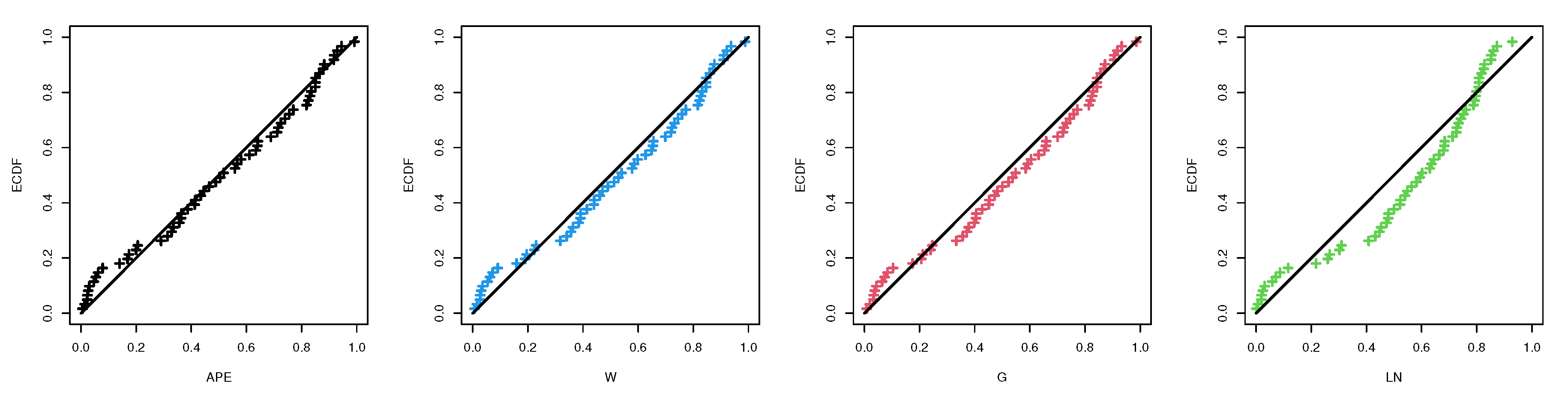
34]. To show the flexibility of the APE distribution, based on the complete electrical appliances dataset, we compare the fit of the APE distribution with three well-known distributions namely: Weibull (W), gamma (G), and log-normal (LN) distributions. For this purpose, different goodness-of-fit measures are employed, such as negative log-likelihood (NL), Akaike (A), Bayesian (B), consistent Akaike (CA), Hannan–Quinn (HQ), Anderson–Darling (A*), and Cramér von Mises (W*) information criteria. Further, for all considered distributions, the Kolmogorov–Smirnov (KS) statistic with its p-value is also computed. The MLEs of the model parameters with their standard errors (SEs), as well as the different model selection criteria, are calculated and reported in 
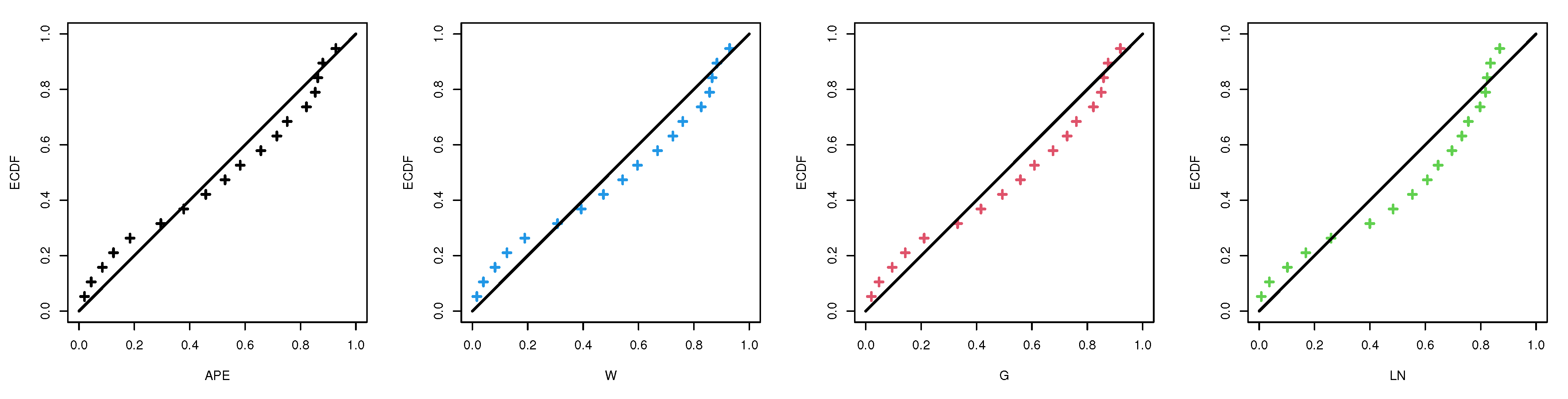
Table 3. The results indicate that the APE distribution provides a better fit than the other distributions because it has the lowest values of all given model selection measures. We also draw quantile–quantile plots of the APE, W, G and LN distributions which are shown in Figure 5. It also supports the same findings. 
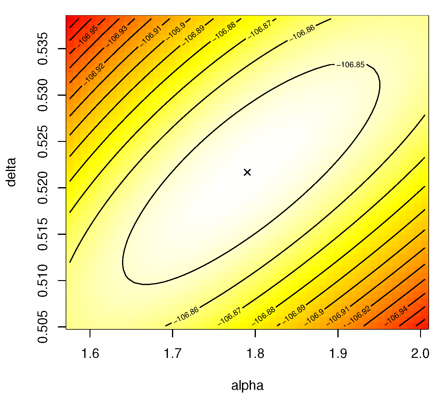
Figure 6 provides the contour plot of the log-likelihood function for α and δ by using the complete electrical appliances dataset. It shows that the best starting values of α and δ are close to 1.7904 and 0.5217, respectively, as well as the fact that it indicates that their MLEs exist and are unique.
Using the complete electrical appliances failure times, we generate a first-failure censored sample after randomly grouping this dataset into 20 groups with k = 3 items within each group and report it in Table 4. Thus, the first-failure censored sample (in order) is: 0.014, 0.034, 0.059, 0.061, 0.069, 0.080, 0.123, 0.142, 0.210, 0.381, 0.464, 0.479, 0.556, 0.574, 0.839, 0.991, 1.088, 1.275, 1.355, and 1.397.
Using this first-failure censored data, three different progressive first-failure censored samples using three different censoring schemes with m = 10 are generated and reported in Table 5. For brevity, the censoring scheme R = ( 2 , 0 , 0 , 0 , 2 ) is denoted by R = ( 2 , 0 3 , 2 ) . For each generated PFFC sample presented in Table 5, we calculating the MLEs with their SEs of α , δ , R ( t ) and h ( t ) (at time t = 0.5 ). 
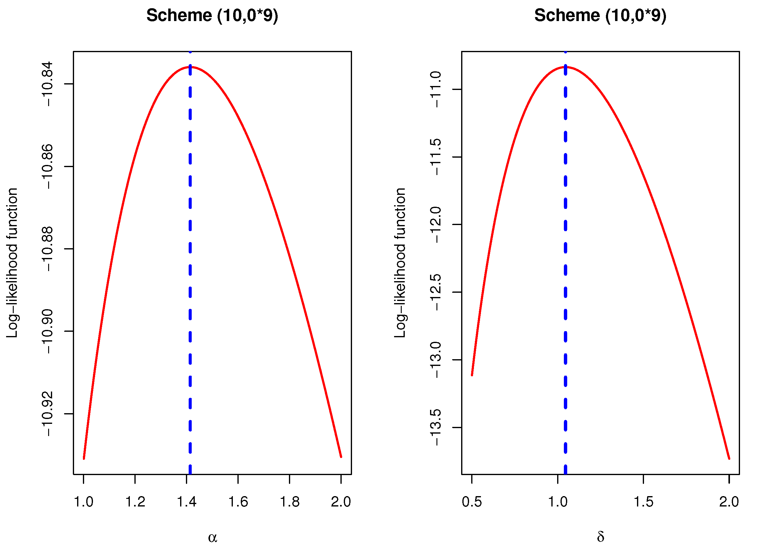
Figure 7 shows the plots of the log-likelihood functions of α and δ for scheme ( 10 , 0 9 ) as an example which shows that the MLEs of α and δ exist and unique.
Via the M-H algorithm sampler, from 30,000 MCMC samples with 5000 burn-in, the Bayes estimates with their SEs of α , δ , R ( t ) , and h ( t ) (at time t = 0.5 ) are developed under SEL and LL (for η ( = 3 , 0.03 , + 3 ) ) functions using non-informative prior. Additionally, the lower and upper bounds of the 95% ACI/HPD credible interval estimates with their interval lengths are also calculated. The MLEs of α and δ are chosen as the initial guesses to apply the M-H algorithm. All point and interval estimates of α , δ , R ( t ) , and h ( t ) are reported in Table 6 and Table 7, respectively. It is clear, from Table 6 and Table 7, that the point estimates of α , δ , R ( t ) , and h ( t ) obtained by both likelihood and Bayesian estimation methods are quite close to each other. A similar pattern is also observed in the case of interval estimation using ACIs and HPD credible intervals.
Using the data in Table 5, the proposed optimum criteria are also computed and provided in Table 8. It shows that the progressive censoring scheme ( 0 9 , 10 ) is the optimal scheme over others for criteria 1, 2, and 3, while the progressive censoring scheme ( 0 5 , 10 , 0 4 ) is the optimal scheme than others for criterion 4.
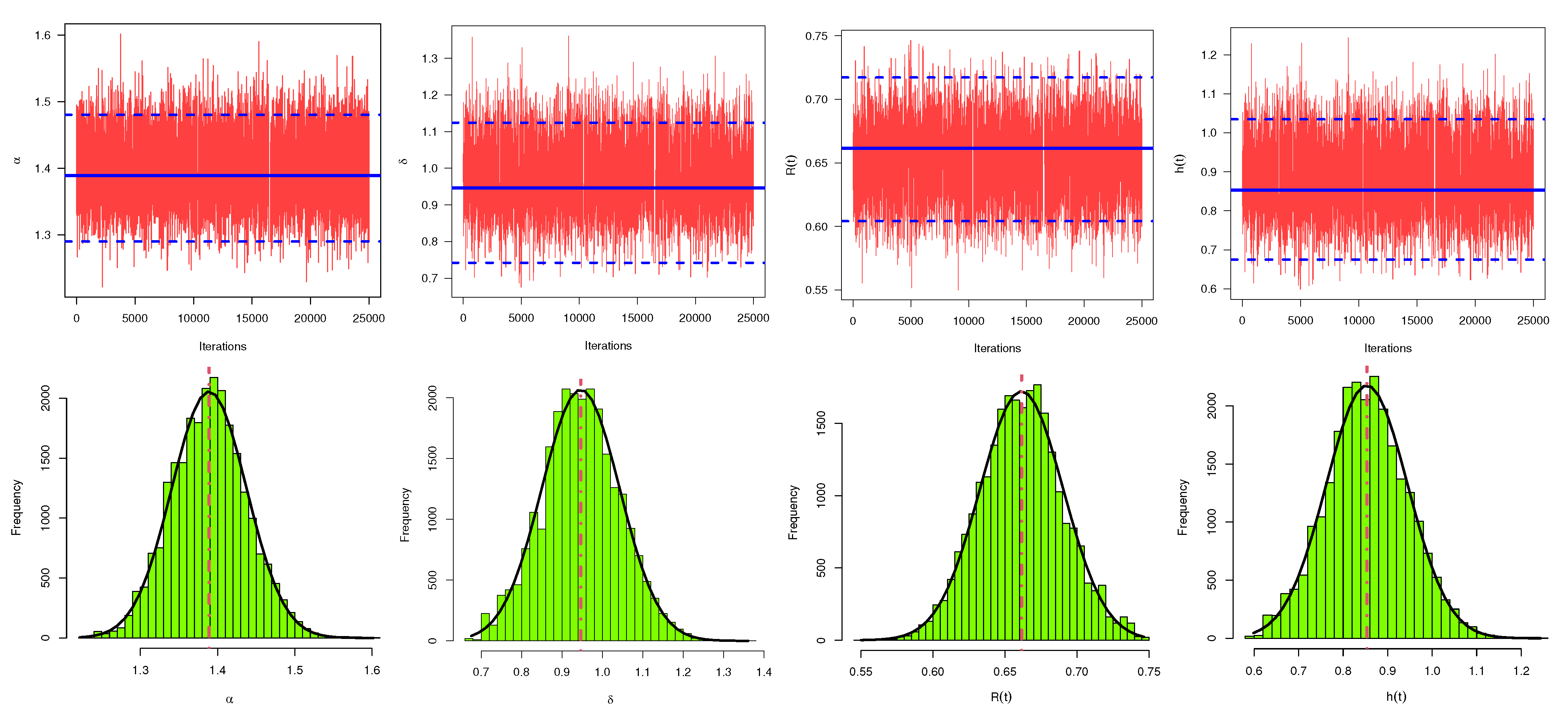
To assess the convergence of MCMC outputs, using the generated sample by censoring scheme ( 10 , 0 9 ) (as an example), trace plots of MCMC simulated variates with their sample mean (horizontal soled line (—)) and two bounds of 95% HPD credible intervals (horizontal dashed lines (- - -)) of α , δ , R ( t ) and h ( t ) are displayed in Figure 8. Additionally, using a Gaussian kernel for the same sample, the histograms of the simulated MCMC estimates with their sample mean (vertical dotted line (:)) of α , δ , R ( t ) , and h ( t ) are also displayed in Figure 8. It shows that the MCMC technique converges very well and it also shows that discarding the first 5000 samples is appropriate size to ignore the effect of the initial values. It can be also seen, from Figure 8, that the simulated MCMC variates of α and δ are fairly symmetrical while the generated posteriors of the R ( t ) and h ( t ) are negative and positive quite skewed, respectively.

6.2. Electronic Devices

The second dataset contains the failure times of 18 electronic devices which are: 5, 11, 21, 31, 46, 75, 98, 122, 145, 165, 196, 224, 245, 293, 321, 330, 350, and 420. This dataset was originally reported by Wang [35], and recently analyzed by Elshahhat and Abu El Azm [36] and Alotaibi et al. [15]. From the complete electronic devices data, the MLEs (along with their SEs) and the model selection criteria (NL, A, B, CA, HQ, A*, W*, and KS) of APE distribution and the other competitive lifetime (W, G, and LN) models are calculated and displayed in Table 9. It shows that the APE distribution fits the electrical appliances data quite well, compared to others. Moreover, the corresponding quantile–quantile plots of the APE distribution and its competing models are displayed in Figure 9. It is evident that the APE distribution is the best choice among all the competing models based on fitting electronic devices data.
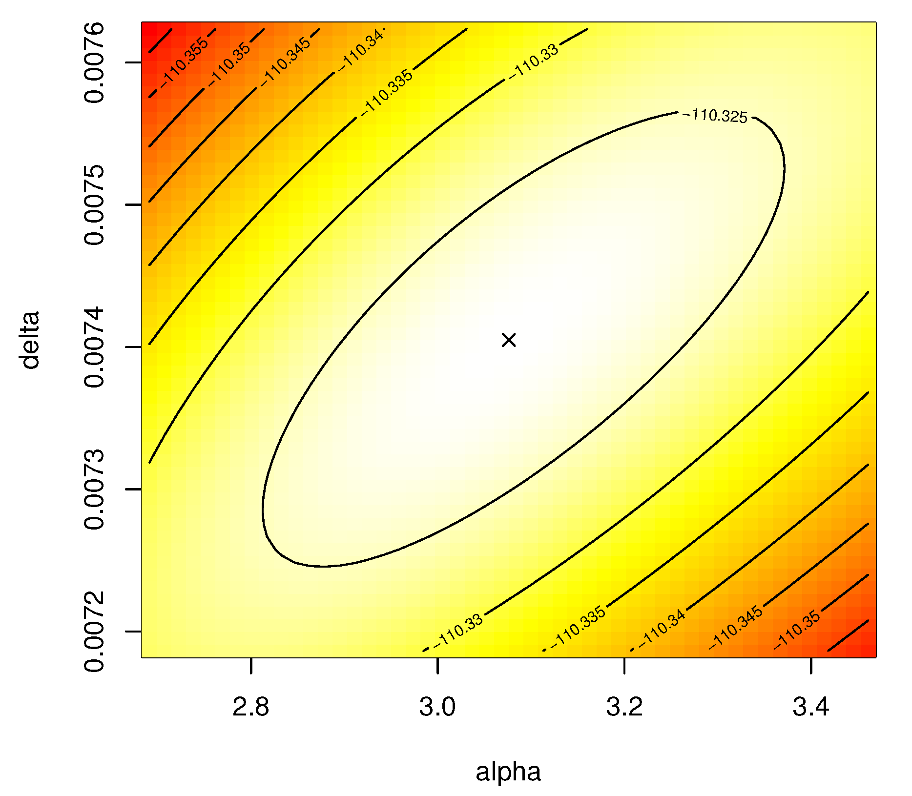
Figure 10 shows that the best initial values of α and δ are close to 3.0761 and 0.0074, respectively, as well as it also indicates that their MLEs exist and are also unique.
Using the complete electronic devices data, one first-failure censored sample is generated by randomly grouping this dataset into 9 groups with k = 2 items within each group, see Table 10. As a result, the first-failure censored sample (in order) is: 5, 11, 21, 31, 46, 75, 98, 165, and 245. Now, three different progressive first-failure censored samples based on three different censoring schemes with m = 5 are generated from the first-failure censored data and are listed in Table 11. For each generated PFFC sample, the maximum likelihood and Bayes M-H estimates with their SEs of α , δ , R ( t ) and h ( t ) (at time t = 10 ) are computed and provided in Table 12. 
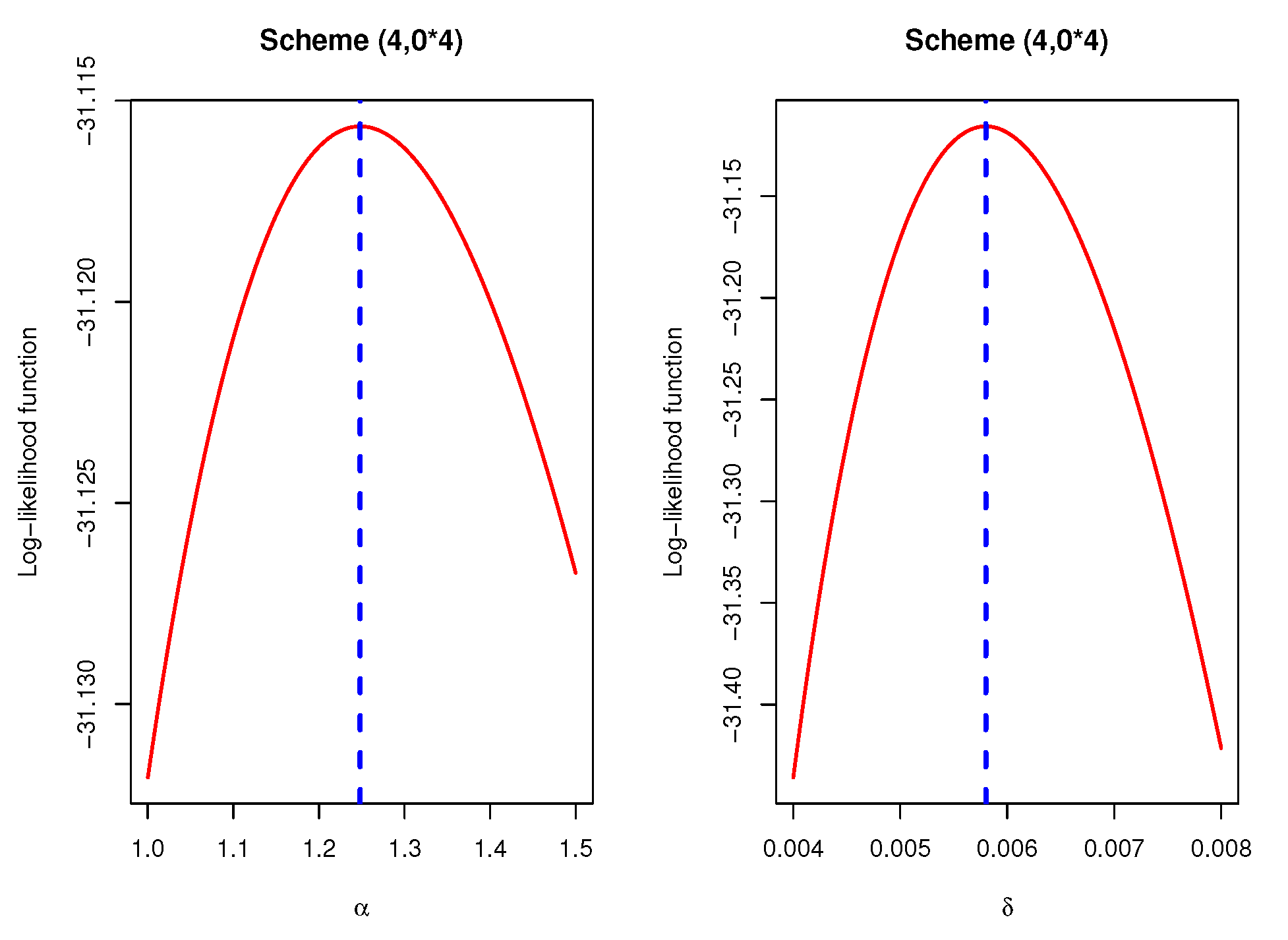
Figure 11 presents the plots of the log-likelihood functions of α and δ for scheme ( 4 , 0 4 ) as an example which shows that the MLEs of α and δ exist and unique.
Using gamma improper priors, based on 30,000 MCMC samples with 5000 burn-in, the MCMC estimates with their SEs of α , δ , R ( t ) and h ( t ) (at time t = 10 ) are developed under SEL and LL (for η ( = 2 , 0.02 , + 2 ) ). Moreover, the two-sided 95% ACI/HPD credible interval estimates with their interval lengths for α , δ , R ( t ) , and h ( t ) are also calculated and reported in Table 13. The calculated values of α ^ and δ ^ are chosen as the initial values to run the M-H algorithm. It is noted, from Table 12 and Table 13, that the statistical inferences of α , δ , R ( t ) , and h ( t ) derived from the Bayesian M-H approach perform better than the maximum likelihood approach in terms of smallest SEs, and the HPD credible interval estimates perform better than asymptotic interval estimates in terms of shortest interval lengths. Furthermore, for each PFFC sample, the proposed optimum criteria are presented in Table 14. It shows that the progressive censoring scheme ( 4 , 0 4 ) is the optimal scheme compared to others for criteria 1, 2, and 3, while the censoring scheme ( 0 4 , 4 ) is the optimal scheme compared to others for criterion 4.
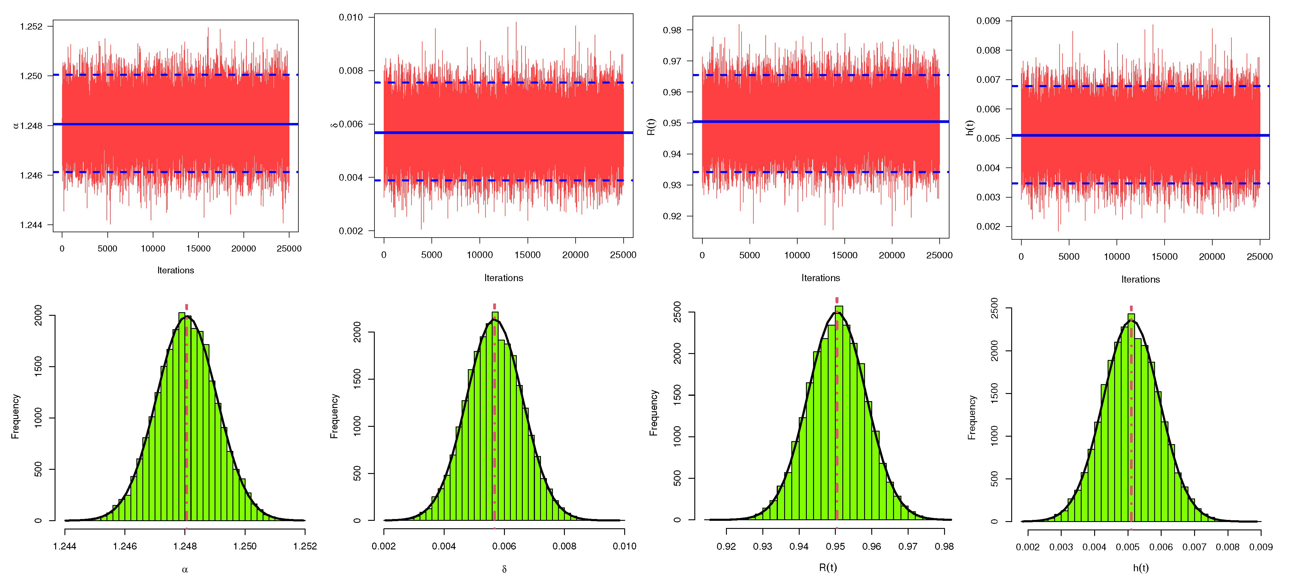
As an example, using the generated sample by censoring scheme ( 4 , 0 4 ) , trace and histogram plots of the MCMC simulated variates of α , δ , R ( t ) , and h ( t ) are provided in Figure 12. It shows that the MCMC mechanism converges well and that the simulated MCMC variates of all unknown parameters are fairly symmetrical. Finally, both numerical results of the proposed methodologies under the complete failure times dataset of electrical appliances and electronic devices provide a good explanation to the proposed model.

7. Concluding Remarks

In this study, we investigate the progressive first-failure censoring scheme under the assumption that the lifetime of the population follows the alpha power exponential distribution. We have used the method of maximum likelihood to obtain the point estimates of the unknown parameters and some reliability characteristics. In addition, the approximate confidence intervals are obtained by utilizing the asymptotic properties of the maximum likelihood estimates. The Bayesian estimation method is employed to acquire the point estimates, as well as the highest posterior density credible intervals. The Bayes estimates are obtained through squared error and LINEX loss function via applying the Monte Carlo Markov Chain technique. Comprehensive simulation experiments are implemented to examine the performance of the different point and interval estimators. We have also delivered various criteria to choose the optimal sampling plan. For applicability purposes, two engineering applications are considered. The outcomes of the simulation study and the two applications revealed that the Bayes estimates perform quite well, even for small sample sizes. The Bayes estimates have the smallest root mean squared error when compared with those based on the classical approach. Additionally, the highest credible density credible intervals perform better than the approximate confidence intervals in terms of minimum interval lengths. It may be said that in this paper, we have proposed the Bayesian estimation using squared error and LINEX loss functions, although most of the outcomes can be developed for any other loss functions.

Supplementary Materials

The following supporting information can be downloaded at: https://www.mdpi.com/article/10.3390/axioms11100553/s1, Table S1: The average estimates (1st row), RMSEs (2nd row) and MRABs (3rd row) of α when k = 2 ; Table S2: The average estimates (1st row), RMSEs (2nd row) and MRABs (3rd row) of α when k = 5 ; Table S3: The average estimates (1st row), RMSEs (2nd row) and MRABs (3rd row) of δ when k = 2 ; Table S4: The average estimates (1st row), RMSEs (2nd row) and MRABs (3rd row) of δ when k = 5 ; Table S5: The average estimates (1st row), RMSEs (2nd row) and MRABs (3rd row) of R ( t ) when k = 2 ; Table S6: The average estimates (1st row), RMSEs (2nd row) and MRABs (3rd row) of R ( t ) when k = 5 ; Table S7: The average estimates (1st row), RMSEs (2nd row) and MRABs (3rd row) of h ( t ) when k = 2 ; Table S8: The average estimates (1st row), RMSEs (2nd row) and MRABs (3rd row) of h ( t ) when k = 5 ; Table S9: The ACLs (1st column) and CPs (2nd column) of ACI/HPD credible intervals of α ; Table S10: The ACLs (1st column) and CPs (2nd column) of ACI/HPD credible intervals of δ ; Table S11: The ACLs (1st column) and CPs (2nd column) of ACI/HPD credible intervals of R ( t ) ; Table S12: The ACLs (1st column) and CPs (2nd column) of ACI/HPD credible intervals of h ( t ) .

Author Contributions

Methodology, A.E. and M.N.; Funding acquisition, R.A.; Software, A.E.; Supervision A.E.; Writing–original draft, R.A. and M.N.; Writing—review and editing M.N. All authors have read and agreed to the published version of the manuscript.

Funding

This research was funded by Princess Nourah bint Abdulrahman University Researchers Supporting Project number (PNURSP2022R50), Princess Nourah bint Abdulrahman University, Riyadh, Saudi Arabia.

Data Availability Statement

The authors confirm that the data supporting the findings of this study are available within the article.

Acknowledgments

The authors would like to express their thanks to the editor and the five anonymous referees for helpful comments and observations. Princess Nourah bint Abdulrahman University Researchers Supporting Project number (PNURSP2022R50), Princess Nourah bint Abdulrahman University, Riyadh, Saudi Arabia.

Conflicts of Interest

The authors declare no conflict of interest.

References

  1. Wu, S.J.; Kuş, C. On estimation based on progressive first-failure-censored sampling. Comput. Stat. Data Anal. 2009, 53, 3659–3670. [Google Scholar] [CrossRef]
  2. Soliman, A.A.; Abd-Ellah, A.H.; Abou-Elheggag, N.A.; Abd-Elmougod, G.A. Estimation of the parameters of life for Gompertz distribution using progressive first-failure censored data. Comput. Stat. Data Anal. 2012, 56, 2471–2485. [Google Scholar] [CrossRef]
  3. Dube, M.; Garg, R.; Krishna, H. On progressively first failure censored Lindley distribution. Comput. Stat. 2016, 31, 139–163. [Google Scholar] [CrossRef]
  4. Ahmed, E.A. Estimation and prediction for the generalized inverted exponential distribution based on progressively first-failure-censored data with application. J. Appl. Stat. 2017, 44, 1576–1608. [Google Scholar] [CrossRef]
  5. Ashour, S.K.; El-Sheikh, A.A.; Elshahhat, A. Maximum likelihood estimation of the generalised Gompertz distribution under progressively first-failure censored sampling. S. Afr. Stat. J. 2018, 52, 115–128. [Google Scholar] [CrossRef]
  6. Ashour, S.K.; El-Sheikh, A.A.; Elshahhat, A. Inferences and optimal censoring schemes for progressively first-failure censored Nadarajah-Haghighi distribution. Sankhya A 2022, 84, 885–923. [Google Scholar] [CrossRef]
  7. Ashour, S.K.; El-Sheikh, A.A.; Elshahhat, A. Inferences for Weibull parameters under progressively first-failure censored data with binomial random removals. Stat. Optim. Inf. Comput. 2021, 9, 47–60. [Google Scholar] [CrossRef]
  8. Shi, X.; Shi, Y. Inference for inverse power Lomax distribution with progressive first-failure censoring. Entropy 2021, 23, 1099. [Google Scholar] [CrossRef]
  9. Xie, Y.; Gui, W. Statistical inference of the lifetime performance index with the log-logistic distribution based on progressive first-failure-censored data. Symmetry 2020, 12, 937. [Google Scholar] [CrossRef]
  10. Saini, S.; Tomer, S.; Garg, R. On the reliability estimation of multicomponent stress–strength model for Burr XII distribution using progressively first-failure censored samples. J. Stat. Comput. Simul. 2022, 92, 667–704. [Google Scholar] [CrossRef]
  11. Cai, Y.; Gui, W. Classical and Bayesian inference for a progressive first-failure censored left-truncated normal distribution. Symmetry 2021, 13, 490. [Google Scholar] [CrossRef]
  12. Mahdavi, A.; Kundu, D. A new method for generating distributions with an application to exponential distribution. Commun. Stat. Theory Methods 2017, 46, 6543–6557. [Google Scholar] [CrossRef]
  13. Nassar, M.; Afify, A.Z.; Shakhatreh, M. Estimation methods of alpha power exponential distribution with applications to engineering and medical data. Pak. J. Stat. Oper. Res. 2020, 16, 149–166. [Google Scholar] [CrossRef]
  14. Salah, M.M. On progressive Type-II censored samples from alpha power exponential distribution. J. Math. 2020, 2020, 2584184. [Google Scholar] [CrossRef]
  15. Alotaibi, R.; Elshahhat, A.; Rezk, H.; Nassar, M. Inferences for Alpha Power Exponential Distribution Using Adaptive Progressively Type-II Hybrid Censored Data with Applications. Symmetry 2022, 14, 651. [Google Scholar] [CrossRef]
  16. Nassar, M.; Alotaibi, R.; Zhang, C. Estimation of Reliability Indices for Alpha Power Exponential Distribution Based on Progressively Censored Competing Risks Data. Mathematics 2022, 10, 2258. [Google Scholar] [CrossRef]
  17. Luo, C.; Shen, L.; Xu, A. Modelling and estimation of system reliability under dynamic operating environments and lifetime ordering constraints. Reliab. Eng. Syst. Saf. 2022, 218, 108136. [Google Scholar] [CrossRef]
  18. Greene, W.H. Econometric Analysis, 4th ed.; Pearson Prentice-Hall: Upper Saddle River, NJ, USA, 2000. [Google Scholar]
  19. Anastasiou, A.; Ley, C. Bounds for the asymptotic normality of the maximum likelihood estimator using the Delta method. Am. J. Probab. Math. Stat. 2017, 14, 153–171. [Google Scholar] [CrossRef]
  20. Anastasiou, A.; Gaunt, R.E. Multivariate normal approximation of the maximum likelihood estimator via the delta method. Braz. J. Probab. Stat. 2020, 34, 136–149. [Google Scholar] [CrossRef] [Green Version]
  21. Henningsen, A.; Toomet, O. maxLik: A package for maximum likelihood estimation in R. Comput. Stat. 2011, 26, 443–458. [Google Scholar] [CrossRef]
  22. Klebanov, L.B. Universal loss function and unbiased estimation. Dokl. Akad. Nank SSSR Soviet Math. Dokl. 1972, 203, 1249–1251. [Google Scholar]
  23. Varian, H.R. A Bayesian Approach to Real Estate Assessment. In Studies in Bayesian Econometrics and Statistics; Savage, L.J., Feinberg, S.E., Zellner, A., Eds.; Honor of L. J. Savage; North-Holland Pub. Co.: Amsterdam, The Netherlands, 1975; pp. 195–208. [Google Scholar]
  24. Basu, A.P.; Ebrahimi, N. Bayesian approach to life testing and reliability estimation using asymmetric loss function. J. Stat. Plan. Inference 1991, 29, 21–31. [Google Scholar] [CrossRef]
  25. Al Sobhi, M.M.A.; Soliman, A.A. Estimation for the exponentiated Weibull model with adaptive Type-II progressive censored schemes. Appl. Math. Model. 2016, 40, 1180–1192. [Google Scholar] [CrossRef]
  26. Wang, Y.; Wang, W.; Tang, Y. A Bayesian semiparametric accelerate failure time mixture cure model. Int. J. Biostat. 2021. [Google Scholar] [CrossRef] [PubMed]
  27. Chen, M.H.; Shao, Q.M. Monte Carlo estimation of Bayesian credible and HPD intervals. J. Comput. Graph. Stat. 1999, 8, 69–92. [Google Scholar]
  28. Plummer, M.; Best, N.; Cowles, K.; Vines, K. CODA: Convergence diagnosis and output analysis for MCMC. R News 2006, 6, 7–11. [Google Scholar]
  29. Meredith, M.; Kruschke, J. R Package ‘HDInterval’: Highest (Posterior) Density Intervals. 2018. Available online: https://CRAN.R-project.org/package=HDInterval (accessed on 3 March 2022).
  30. Balakrishnan, N.; Aggarwala, R. Progressive Censoring, Theory, Methods and Applications; Birkhauser: Boston, MA, USA, 2000. [Google Scholar]
  31. Balasooriya, U.; Balakrishnan, N. Reliability sampling plans for log-normal distribution based on progressively-censored samples. IEEE Trans. Reliab. 2000, 49, 199–203. [Google Scholar] [CrossRef]
  32. Pradhan, B.; Kundu, D. On progressively censored generalized exponential distribution. Test 2009, 18, 497–515. [Google Scholar] [CrossRef]
  33. Lawless, J.F. textitStatistical Models and Methods For Lifetime Data, 2nd ed.; John Wiley and Sons.: Hoboken, NJ, USA, 2011. [Google Scholar]
  34. Dey, S.; Elshahhat, A. Analysis of Wilson-Hilferty distribution under progressive Type-II censoring. Qual. Reliab. Eng. Int. 2022. [Google Scholar] [CrossRef]
  35. Wang, F.K. A new model with bathtub-shaped failure rate using an additive Burr XII distribution. Reliab. Eng. Syst. Saf. 2000, 70, 305–312. [Google Scholar] [CrossRef]
  36. Elshahhat, A.; Abu El Azm, W.S. Statistical reliability analysis of electronic devices using generalized progressively hybrid censoring plan. Qual. Reliab. Eng. Int. 2022, 38, 1112–1130. [Google Scholar] [CrossRef]
Figure 1. Heatmap plots for classical and Bayesian estimation results of α .
Axioms 11 00553 g001
Figure 2. Heatmap plots for classical and Bayesian estimation results of δ .
Axioms 11 00553 g002
Figure 3. Heatmap plots for classical and Bayesian estimation results of R ( t ) .
Axioms 11 00553 g003
Figure 4. Heatmap plots for classical and Bayesian estimation results of h ( t ) .
Axioms 11 00553 g004
Figure 5. The quantile–quantile plot of the APE distribution and other competing models from electrical appliances data.
Axioms 11 00553 g005
Figure 6. Contour plot of α and δ under electrical appliances data.
Axioms 11 00553 g006
Figure 7. The log-likelihood functions of α and δ using scheme ( 10 , 0 9 ) for electrical appliances data.
Axioms 11 00553 g007
Figure 8. Trace (top-panel) and histograms (bottom-panel) plots of α , δ , R ( t ) , and h ( t ) from electrical appliances data.
Axioms 11 00553 g008
Figure 9. The quantile–quantile plot of the APE distribution and other competing models from electronic devices data.
Axioms 11 00553 g009
Figure 10. Contour plot of α and δ under electronic devices data.
Axioms 11 00553 g010
Figure 11. The log-likelihood functions of α and δ using scheme ( 4 , 0 4 ) for electronic devices data.
Axioms 11 00553 g011
Figure 12. Trace (top-panel) and Histograms (bottom-panel) plots of α , δ , R ( t ) and h ( t ) from electronic devices data.
Axioms 11 00553 g012
Table 1. Some optimal criteria.
CriterionObjective
1 Maximize trace [ I ( α ^ , δ ^ ) ]
2 Minimize trace [ I 1 ( α ^ , δ ^ ) ]
3 Minimize det [ I 1 ( α ^ , δ ^ ) ]
4 Minimize v a r ( log ( ξ ^ q ) )
Table 2. Time points of 60 electrical appliances.
0.0140.0340.0590.0610.0690.0800.1230.1420.1650.210
0.3810.4640.4790.5560.5740.8390.9170.9690.9911.064
1.0881.0911.1741.2701.2751.3551.3971.4771.5781.649
1.7021.8931.9322.0012.1612.2922.3262.3372.6282.785
2.8112.8862.9933.1223.2483.7153.7903.8573.9124.100
4.1064.1164.3154.5104.5805.2675.2995.5836.0659.701
Table 3. Summary fit of the APE distribution and other competing models under electrical appliances data.
ModelMLE (SE)NLABCAHQA*W*KS
α δ Distancep-Value
APE1.7893 (1.3408)0.5216 (0.1034)106.843217.687221.875217.897219.3250.57920.08080.08780.7104
W1.0009 (0.1066)0.4555 (0.0814)107.115218.231222.419218.441219.8690.71540.10370.07770.8432
G0.9307 (0.1487)0.4244 (0.0884)107.012218.235222.213218.235219.6630.71840.10420.08970.6861
LN0.1597 (0.1858)1.4392 (0.1314)116.565237.129241.318237.339238.7672.52410.42920.16540.0667
Table 4. Random grouping for the electrical appliances dataset.
Group Item12345678910
1.8933.9124.1061.1744.3150.839 *1.397 *3.8571.355 *1.088 *
0.556 *0.9692.3260.069 *0.034 *1.6495.2672.1612.3374.100
2.6280.059 *1.275 *1.9325.2992.2922.0010.014 *6.0652.886
Group Item11121314151617181920
3.7902.8110.464 *0.080 *0.9174.1160.061 *1.7021.4770.165
1.0640.479 *1.0914.5100.574 *1.2704.5803.2481.5780.142 *
0.991 *9.7012.9933.1225.5830.381 *3.7150.123 *0.210 *2.785
Note: The starred number is the first-failure item in each group.
Table 5. Three different PFFC samples from the electrical appliances dataset.
SchemeGenerated Censored Sample
( 10 , 0 9 ) 0.014, 0.061, 0.069, 0.123, 0.142, 0.210, 0.464, 0.574, 0.839, 0.991
( 0 5 , 10 , 0 4 ) 0.014, 0.034, 0.059, 0.061, 0.069, 0.080, 0.142, 0.464, 0.574, 0.839
( 0 9 , 10 ) 0.014, 0.034, 0.059, 0.061, 0.069, 0.080, 0.123, 0.142, 0.210, 0.381
Table 6. The point estimates (SEs) of α , δ , R ( t ) , and h ( t ) using electrical appliances data.
SchemeParameterMLESELLL
η −3−0.03+3
( 10 , 0 9 ) α 1.4143 (3.6763)1.3890 (0.0003)1.3925 (0.0218)1.3890 (0.0253)1.3855 (0.0288)
δ 1.0457 (1.0386)0.9464 (0.0006)0.9604 (0.0854)0.9465 (0.0992)0.9325 (0.1133)
R ( 0.5 ) 0.6341 (0.0938)0.6615 (0.0002)0.6627 (0.0286)0.6615 (0.0274)0.6602 (0.0261)
h ( 0.5 ) 0.9420 (0.3574)0.8533 (0.0006)0.8660 (0.0760)0.8535 (0.0885)0.8408 (0.1012)
( 0 5 , 10 , 0 4 ) α 1.2658 (3.2983)1.2405 (0.0003)1.2442 (0.0215)1.2406 (0.0252)1.2369 (0.0289)
δ 1.1686 (1.2678)1.0723 (0.0006)1.0858 (0.0828)1.0724 (0.0961)1.0590 (0.1096)
R ( 0.5 ) 0.5864 (0.1007)0.6114 (0.0002)0.6126 (0.0262)0.6114 (0.0250)0.6103 (0.0239)
h ( 0.5 ) 1.0935 (0.5109)1.0066 (0.0006)1.0196 (0.0739)1.0067 (0.0867)0.9938 (0.0996)
( 0 9 , 10 ) α 0.1514 (0.9670)0.1502 (0.0001)0.1504 (0.0009)0.1502 (0.0011)0.1501 (0.0013)
δ 0.3144 (0.7126)0.3001 (0.0003)0.3030 (0.0113)0.3000 (0.0143)0.2970 (0.0173)
R ( 0.5 ) 0.7170 (1.0215)0.7277 (0.0002)0.7294 (0.0124)0.7278 (0.0107)0.7260 (0.0090)
h ( 0.5 ) 0.6333 (7.1874)0.6078 (0.0005)0.6182 (0.0151)0.0107 (0.0253)0.5973 (0.0359)
Table 7. The interval estimates [lengths] of α , δ , R ( t ) and h ( t ) using electrical appliances data.
SchemeParameterACIHPD
( 10 , 0 9 ) α (0.0000,8.6197) [8.6197](1.2902,1.4803) [0.1901]
δ (0.0000,3.0813) [3.0813](0.7420,1.1241) [0.3821]
R ( 0.5 ) (0.4503,0.8179) [0.3676](0.6041,0.7172) [0.1131]
h ( 0.5 ) (0.2415,1.6423) [1.4008](0.6049,1.0347) [0.3598]
α (0.0000,7.7303) [7.7303](1.1463,1.3409) [0.1946]
( 0 5 , 10 , 0 4 ) δ (0.0000,3.6534) [3.6534](0.8910,1.2602) [0.3692]
R ( 0.5 ) (0.3890,0.7838) [0.3948](0.5579,0.6655) [0.1076]
h ( 0.5 ) (0.0921,2.0948) [2.0027](0.8216,1.1833) [0.3617]
( 0 9 , 10 ) α (0.0000,0.7126) [0.7126](0.1308,0.1699) [0.0391]
δ (0.0000,1.7111) [1.7111](0.2142,0.3898) [0.1755]
R ( 0.5 ) (0.0000,0.9999) [0.9999](0.6614,0.7916) [0.1302]
h ( 0.5 ) (0.0000,14.720) [14.720](0.4424,0.7678) [0.3254]
Table 8. Optimal progressive censoring from electrical appliances data.
SchemeCriterion
1234
q 0.3 0.6 0.9
( 10 , 0 9 ) 10.622614.59381.373850.017390.109481.80970
( 0 5 , 10 , 0 4 ) 8.7343512.48611.429540.011220.103831.75503
( 0 9 , 10 ) 146.0021.442930.009880.030960.246035.31991
Table 9. Summary fit of the APE distribution and other competing models under electronic devices data.
ModelMLE (SE)NLABCAHQA*W*KS
α δ Distancep-Value
APE3.0805 (3.8591)0.0074 (0.0021)110.322224.645226.445225.445224.8910.33650.04870.10350.9794
W1.1458 (0.0702)0.0026 (0.0008)110.446224.892226.673225.692225.1380.36490.05390.11320.9550
G1.1156 (0.3214)0.0065 (0.0023)110.603225.207226.987226.007225.4520.39740.05970.12080.9274
LN4.6358 (0.2952)1.2523 (0.2087)230.313230.068231.849230.868230.3130.79490.13130.16460.6553
Table 10. Random grouping for the electronic devices dataset.
Group Item123456789
75 *21 *3505 *330245 *31 *165 *224
19629311 *12246 *42014532198 *
Note: The starred number is the first-failure item in each group.
Table 11. Three different PFFC samples from electronic devices dataset.
SchemeGenerated Censored Sample
( 4 , 0 4 ) 5, 21, 75, 98, 245
( 0 2 , 4 , 0 2 ) 5, 11, 21, 98, 165
( 0 4 , 4 ) 5, 11, 21, 31, 46
Table 12. The point estimates (SEs) of α , δ , R ( t ) , and h ( t ) using electronic devices data.
SchemeParameterMLESELLL
η 2 0.02 + 2
( 4 , 0 4 ) α 1.2481 (0.41   ×   10 + 1 )1.2481 (6.34   ×   10 6 )1.2481 (8.02   ×   10 6 )1.2481 (9.51   ×   10 6 )1.2481 (1.10   ×   10 5 )
δ 0.0058 (6.64   ×   10 3 )0.0057 (5.90   ×   10 6 )0.0057 (1.21   ×   10 4 )0.0057 (1.22   ×   10 4 )0.0057 (1.23   ×   10 4 )
R ( 10 ) 0.9494 (3.59   ×   10 2 )0.9504 (5.04   ×   10 5 )0.9505 (1.17   ×   10 3 )0.9504 (1.07   ×   10 3 )0.9503 (9.75   ×   10 4 )
h ( 10 ) 0.0052 (3.58   ×   10 3 )0.0051 (5.34   ×   10 6 )0.0051 (1.08   ×   10 4 )0.0051 (1.09   ×   10 4 )0.0051 (1.11   ×   10 4 )
( 0 2 , 4 , 0 2 ) α 1.6654 (0.43   ×   10 + 1 )1.6653 (6.32   ×   10 6 )1.6653 (1.87   ×   10 5 )1.6653 (2.02   ×   10 5 )1.6653 (2.17   ×   10 5 )
δ 0.0078 (7.64   ×   10 3 )0.0077 (6.13   ×   10 6 )0.0077 (1.13   ×   10 4 )0.0077 (1.15   ×   10 4 )0.0077 (1.16   ×   10 4 )
R ( 10 ) 0.9413 (3.63   ×   10 2 )0.9422 (4.52   ×   10 5 )0.9423 (9.40   ×   10 4 )0.9422 (8.64   ×   10 4 )0.9421 (7.87   ×   10 4 )
h ( 10 ) 0.0061 (3.63   ×   10 3 )0.0060 (4.89   ×   10 6 )0.0060 (8.88   ×   10 5 )0.0060 (8.97   ×   10 5 )0.0060 (9.06   ×   10 5 )
( 0 4 , 4 ) α 5.5065 (0.83   ×   10 + 1 )5.5064 (1.27   ×   10 5 )5.5064 (4.09   ×   10 5 )5.5065 (4.69   ×   10 5 )5.5064 (5.31   ×   10 5 )
δ 0.0165 (1.03   ×   10 2 )0.0163 (1.21   ×   10 5 )0.0163 (1.58   ×   10 4 )0.0163 (1.64   ×   10 4 )0.0163 (1.69   ×   10 4 )
R ( 10 ) 0.9342 (9.38   ×   10 2 )0.9349 (5.01   ×   10 5 )0.9350 (8.01   ×   10 4 )0.9349 (7.08   ×   10 4 )0.9349 (6.13   ×   10 4 )
h ( 10 ) 0.0073 (4.41   ×   10 3 )0.0072 (6.15   ×   10 6 )0.0073 (2.00   ×   10 5 )0.0073 (2.14   ×   10 5 )0.0073 (2.28   ×   10 5 )
Table 13. The interval estimates [lengths] of α , δ , R ( t ) , and h ( t ) using electronic devices data.
SchemeParameterACIHPD
( 4 , 0 4 ) α (0.0000,9.2399) [9.2399](1.2461,1.2500) [0.0039]
δ (0.0000,0.0188) [0.0188](0.0039,0.0075) [0.0036]
R ( 10 ) (0.8790,0.9926) [0.1136](0.9342,0.9655) [0.0313]
h ( 10 ) (0.0000,0.0122) [0.0122](0.0035,0.0068) [0.0033]
( 0 2 , 4 , 0 2 ) α (0.0000,10.242) [10.242](1.6634,1.6672) [0.0038]
δ (0.0000,0.0227) [0.0227](0.0057,0.0095) [0.0039]
R ( 10 ) (0.8702,0.9174) [0.0472](0.9284,0.9564) [0.0280]
h ( 10 ) (0.0000,0.0132] [0.0132](0.0045,0.0075) [0.0030]
( 0 4 , 4 ) α (0.0000,21.885) [21.885](5.5023,5.5102) [0.0079]
δ (0.0037,0.0367) [0.0330](0.0127,0.0201) [0.0074]
R ( 10 ) (0.7502,0.9796) [0.2294](0.9189,0.9499) [0.0309]
h ( 10 ) (0.0013,0.0160) [0.0147](0.0054,0.0092) [0.0038]
Table 14. Optimal progressive censoring from electronic devices data.
SchemeCriterion
1234
q 0.3 0.6 0.9
( 4 , 0 4 ) 156,546.516.626440.0001061299.1155494.97168,831.01
( 0 2 , 4 , 0 2 ) 92,123.2519.148760.000208697.80173586.00938,945.58
( 0 4 , 4 ) 27,934.8069.835110.002499233.49471288.7227908.135
Publisher’s Note: MDPI stays neutral with regard to jurisdictional claims in published maps and institutional affiliations.

