
Stability Analysis of Delayed COVID-19 Models


Abstract
:1. Introduction
2. The Delayed SEIQRP Model
2.1. The Normalized Delayed Model
2.2. Equilibrium Points and the Basic Reproduction Number
2.3. Stability of the Normalized Delayed Model
- (i)
- Let . In this case, the Equation (10) becomesWe need to prove that all roots of the characteristic Equation (11) have negative real parts. It is easy to see that , and are roots of Equation (11) and all of them are real negative roots. Thus, we just need to analyze the fourth term of (11), here denoted by , that is,Using the Routh–Hurwitz criterion [38], we know that all roots of have negative real parts if, and only if, the coefficients of are strictly positive. In this case, we have andTherefore, we have just proved that the disease free equilibrium, , is locally asymptotically stable for , whenever .
- (ii)
- Let . In this case, we will use Rouché’s theorem [39,40] to prove that all roots of the characteristic Equation (10) cannot intersect the imaginary axis, i.e., the characteristic equation cannot have pure imaginary roots. Suppose the contrary, that is, suppose there exists such that is a solution of (10). Replacing y in the fourth term of (10), we get thatThen,By adding up the squares of both equations, and using the fundamental trigonometric formula, we obtain thatwhich is equivalent toIf , then , andso thatHence, we have , which is a contradiction. Therefore, we have proved that whenever , the characteristic Equation (10) cannot have pure imaginary roots and the disease free equilibrium is locally asymptotically stable, for any strictly positive time-delay .
- (iii)
- Suppose now that . We know that the characteristic Equation (10) has three real negative roots , , and . Thus, we need to check if the remaining roots ofhave negative real parts. It is easy to see that because we are assuming . On the other hand, . Therefore, by continuity of , there is at least one positive root of the characteristic Equation (10). Hence, we conclude that is unstable when .
- (i)
- Let . In this case, the Equation (16) becomeswhere , and . We need to prove that all the roots of the characteristic Equation (17) have negative real parts. It is easy to see that and are roots of (17) and both are real negative roots. Thus, we just need to consider the third term of the above equation. LetUsing the Routh–Hurwitz criterion [38], we know that all roots of have negative real parts if, and only if, the coefficients of are strictly positive and . If , then
- (ii)
- Let . Using Rouché’s theorem, we prove that all the roots of the characteristic Equation (16) cannot intersect the imaginary axis, i.e., the characteristic equation cannot have pure imaginary roots. Suppose the opposite, that is, assume there exists such that is a solution of (16). Replacing y into the third term of (16), we get thatThen,By adding up the squares of both equations, and using the fundamental trigonometric formula, we obtain thatwhereAssume that the basic reproduction number satisfies relations (14) and (15) with the following condition:Then,In contrast, if satisfies relations (14) and (15) with the conditionthen we havewhich is equivalent toThus,Under the assumption that the basic reproduction number satisfies relations (14) and (15), we haveTherefore, if we assume that the basic reproduction number satisfies relations (14) and (15) with condition (20), thenif satisfies relations (14) and (15) with condition (19), then we havewhich is equivalent toand also equivalent toThus,We conclude that the left hand-side of equation (16) is strictly positive, which implies that this equation is not possible. Therefore, (17) does not have imaginary roots, which implies that is locally asymptotically stable for any time delay .
3. The Delayed SEIQRPW Model with Vaccination
3.1. Normalized Delayed Model with Vaccination
3.2. Equilibrium Points and the Basic Reproduction Number
3.3. Stability of the Normalized Delayed Model with Vaccination
- (i)
- Let . In this case, the Equation (30) becomesWe need to prove that all roots of the characteristic Equation (31) have negative real parts. It is easy to see that , and are roots of Equation (31) and the three are real and negative. Thus, we just need to consider the fourth term of Equation (31). LetUsing the Routh–Hurwitz criterion [38], we know that all roots of have negative real parts if, and only if, the coefficients of are strictly positive. In this case, andTherefore, we have proved that the disease free equilibrium, , is locally asymptotically stable for , whenever .
- (ii)
- Let . Using Rouché’s theorem, we prove that all roots of the characteristic Equation (30) cannot have pure imaginary roots. Suppose the contrary, i.e., that there exists such that is a solution of (30). Replacing y in the fourth term of (30), we getThen,By adding up the squares of both equations and using the fundamental trigonometric formula, one haswhich is equivalent toIf , then , andso thatHence, we have which is a contradiction. Therefore, we have proved that if , then the characteristic Equation (30) cannot have pure imaginary roots and the disease free equilibrium is locally asymptotically stable, for any strictly positive time delay .
- (iii)
- Suppose now that . We know that the characteristic Equation (30) has three real negative roots and Thus, we need to check if the remaining roots ofhave negative real parts. It is easy to see that , because we are assuming . On the other hand, . Therefore, by continuity of , there is at least one positive root of the characteristic Equation (30). Hence, we conclude that is unstable, for any .
- (i)
- Let . In this case, Equation (37) becomeswhere , and . Looking at the roots of the characteristic Equation (38), it is easy to see that and are real negative roots of (38). Considering the third term of the above equation, letUsing the Routh–Hurwitz criterion [38], we know that all roots of have negative real parts if, and only if, the coefficients of are strictly positive andIf , then
- (ii)
- Let . By Rouché’s theorem, we prove that all roots of the characteristic Equation (37) cannot intersect the imaginary axis, i.e., the characteristic equation cannot have pure imaginary roots. Suppose the opposite, i.e., that there exists such that is a solution of (37). Replacing y in the third term of (37), we getThen,By adding up the squares of both equations and using the fundamental trigonometric formula, we obtain thatwhereAssume that the basic reproduction number satisfies relations (34) and (35) with the conditionThen,In contrast, if satisfies relations (34) and (35) under the conditionthen we havewhich is equivalent toThus,Under the assumption that the basic reproduction number satisfies relations (34) and (35), we haveTherefore, if we assume that the basic reproduction number satisfies relations (34) and (35) with condition (41), thenif satisfies (34) and (35) with condition (40), then we havewhich is equivalent toand also equivalent toThus,We have just proved that the left hand-side of Equation (37) is strictly positive, which implies that this equation is not possible. Therefore, (38) does not have imaginary roots, and is locally asymptotically stable, for any time delay , whenever satisfies conditions (34) and (35).
4. Numerical Simulations and Discussion
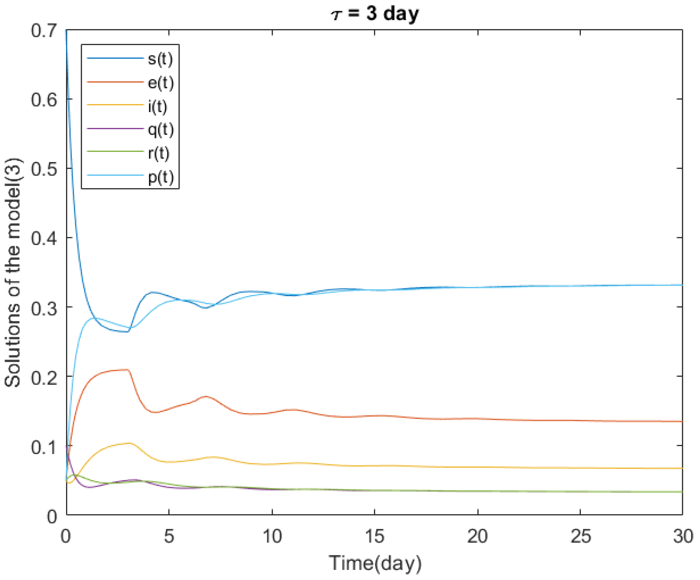
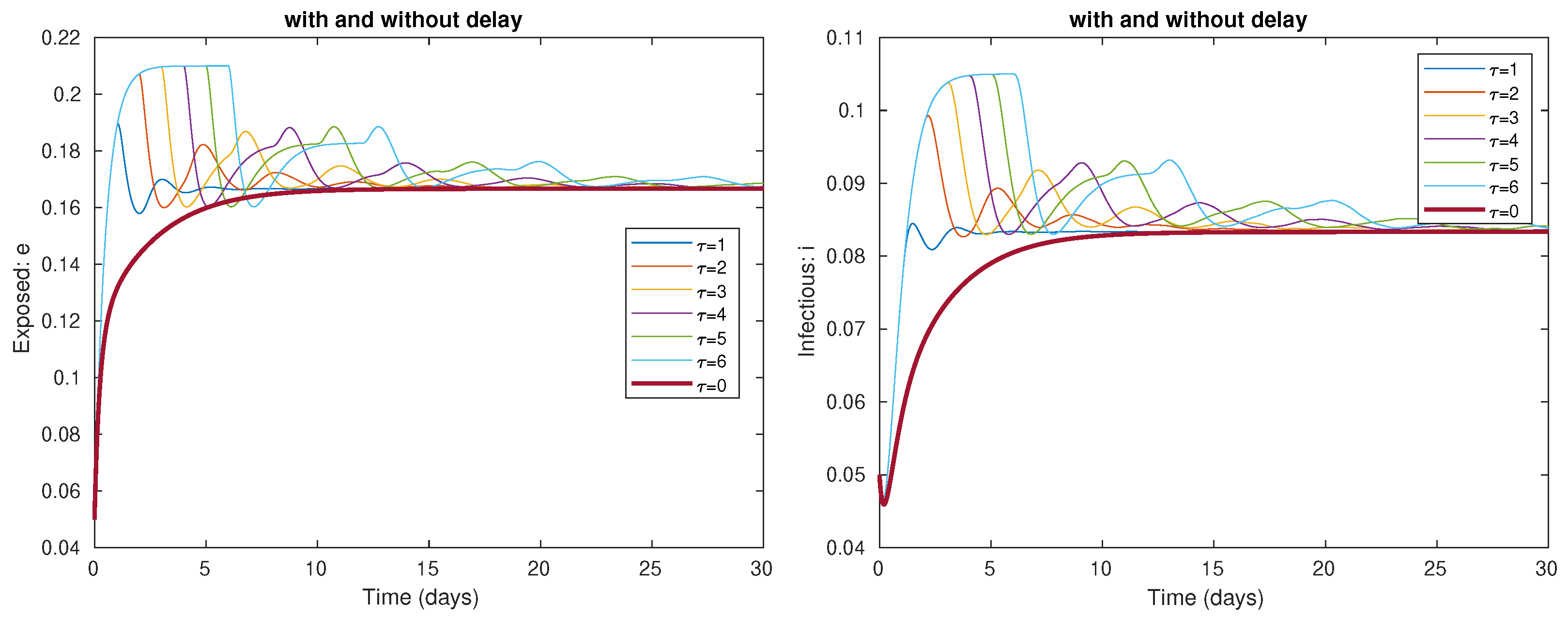
4.1. Local Stability of the Delayed Model
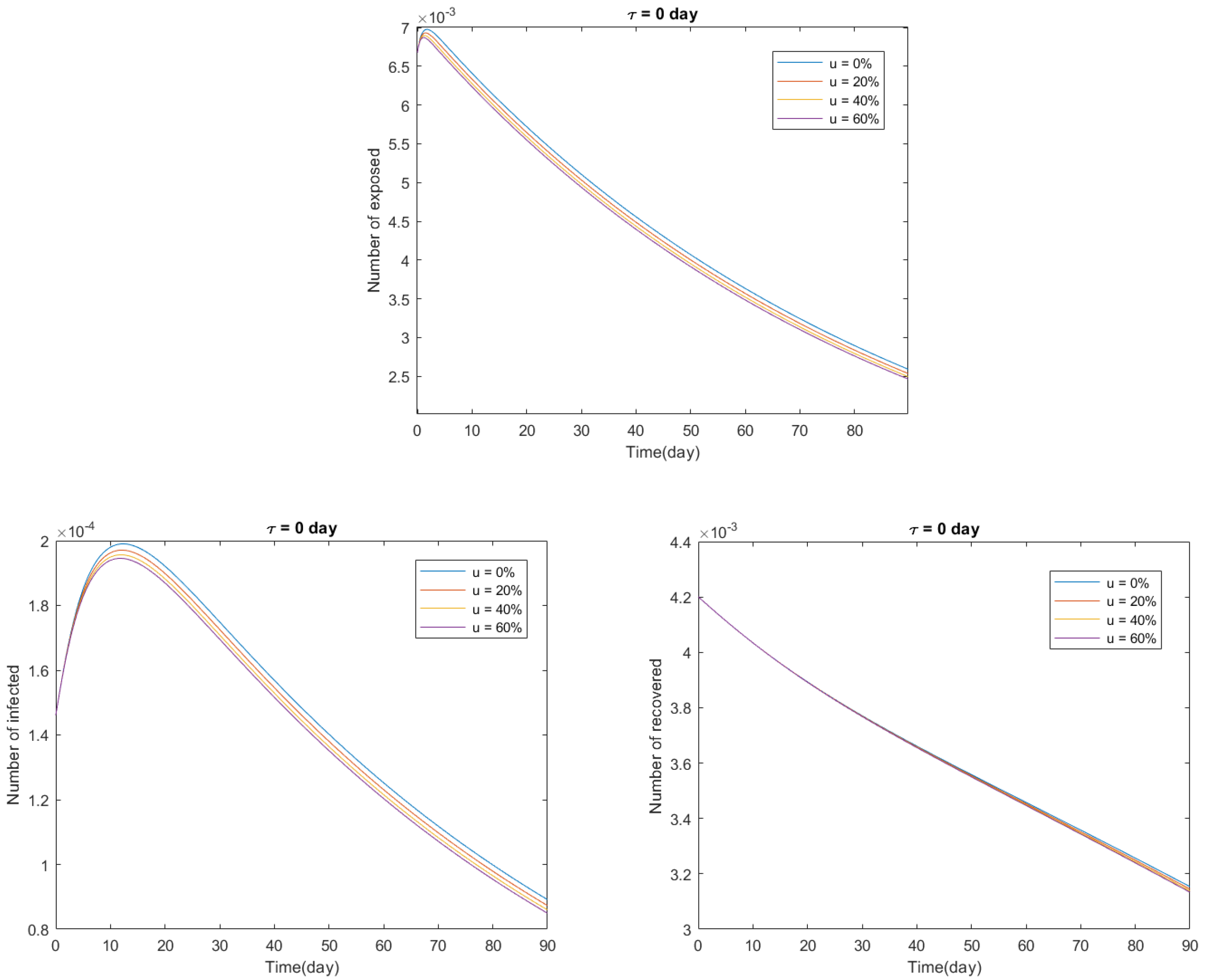
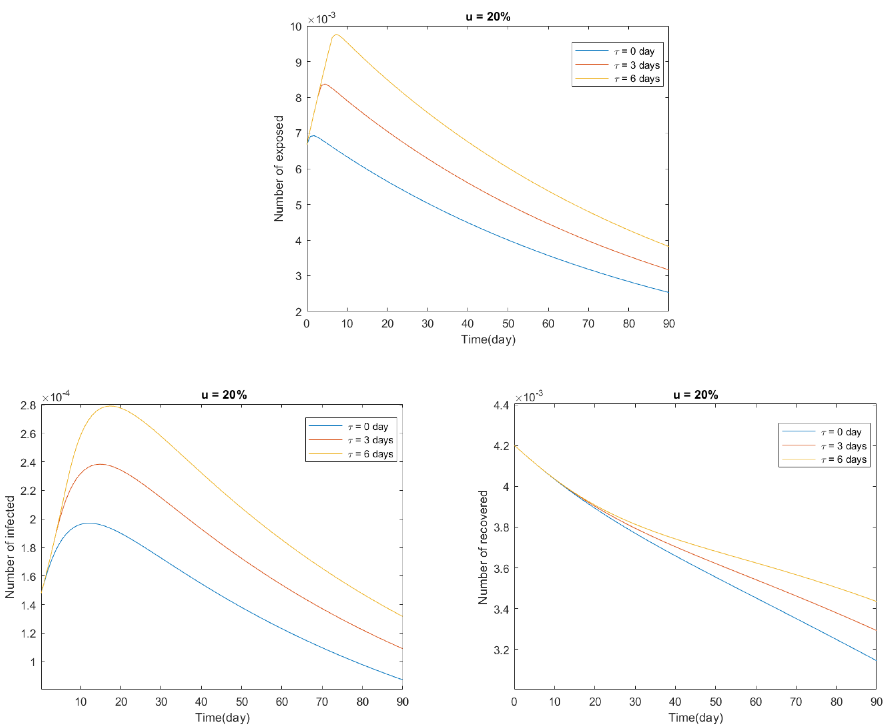
4.2. Delayed Model with Vaccination: COVID-19 in Italy
Author Contributions
Funding
Institutional Review Board Statement
Informed Consent Statement
Data Availability Statement
Acknowledgments
Conflicts of Interest
References
- Porta, M. A Dictionary of Epidemiology; Oxford University Press: Oxford, UK, 2014. [Google Scholar] [CrossRef]
- WHO, World Health Organization. Available online: http://www.emro.who.int/pandemic-epidemic-diseases/outbreaks/index.html (accessed on 29 December 2021).
- WHO, World Health Organization. Available online: https://www.who.int/health-topics/hiv-aids (accessed on 29 December 2021).
- WHO, World Health Organization. Available online: https://www.who.int/health-topics/tuberculosis (accessed on 29 December 2021).
- Lai, C.-C.; Shih, T.P.; Ko, W.C.; Tang, H.J.; Hsueh, P.R. Severe acute respiratory syndrome coronavirus 2 (SARS-CoV-2) and coronavirus disease-2019 (COVID-19): The epidemic and the challenges. Int. J. Antimicrob. Agents 2020, 55, 105924. [Google Scholar] [CrossRef] [PubMed]
- Wang, L.; Wang, Y.; Ye, D.; Liu, Q. Review of the 2019 novel coronavirus (SARS-CoV-2) based on current evidence. Int. J. Antimicrob. Agents 2020, 55, 105948, Erratum in Int. J. Antimicrob. Agents 2020, 56, 106137. [Google Scholar] [CrossRef] [PubMed]
- WHO, World Health Organization. WHO Director-General’s Opening Remarks at the Media Briefing on COVID-19. 11 March 2020. Available online: https://www.who.int/director-general/speeches/detail/who-director-general-s-opening-remarks-at-the-media-briefing-on-covid-19---11-march-2020 (accessed on 29 December 2021).
- Cappi, R.; Casini, L.; Tosi, D.; Roccetti, M. Questioning the seasonality of SARS-COV-2: A Fourier spectral analysis. BMJ Open 2022, 12, e061602. [Google Scholar] [CrossRef] [PubMed]
- Davis, J.T.; Chinazzi, M.; Perra, N.; Mu, K.; y Piontti, A.P.; Ajelli, M.; Dean, N.E.; Gioannini, C.; Litvinova, M.; Merler, S.; et al. Cryptic transmission of SARS-CoV-2 and the first COVID-19 wave. Nature 2021, 600, 127–132. [Google Scholar] [CrossRef]
- Lemos-Paião, A.P.; Silva, C.J.; Torres, D.F.M. A new compartmental epidemiological model for COVID-19 with a case study of Portugal. Ecol. Complex. 2020, 44, 100885. [Google Scholar] [CrossRef]
- Ndaïrou, F.; Area, I.; Nieto, J.J.; Silva, C.J.; Torres, D.F.M. Fractional model of COVID-19 applied to Galicia, Spain and Portugal. Chaos Solitons Fractals 2021, 144, 110652. [Google Scholar] [CrossRef]
- Silva, C.J.; Cruz, C.; Torres, D.F.M.; Muñuzuri, A.P.; Carballosa, A.; Area, I.; Nieto, J.J.; Fonseca-Pinto, R.; Passadouro, R.; Soares dos Santos, E.; et al. Optimal control of the COVID-19 pandemic: Controlled sanitary deconfinement in Portugal. Sci. Rep. 2021, 11, 3451. [Google Scholar] [CrossRef] [PubMed]
- Tang, Y.; Serdan, T.D.A.; Alecrim, A.L.; Souza, D.R.; Nacano, B.R.M.; Silva, F.L.R.; Silva, E.B.; Poma, S.O.; Gennari-Felipe, M.; Iser-Bem, P.N.; et al. A simple mathematical model for the evaluation of the long first wave of the COVID-19 pandemic in Brazil. Sci. Rep. 2021, 11, 16400. [Google Scholar] [CrossRef] [PubMed]
- Zine, H.; Boukhouima, A.; Lotfi, E.M.; Mahrouf, M.; Torres, D.F.M.; Yousfi, N. A stochastic time-delayed model for the effectiveness of Moroccan COVID-19 deconfinement strategy. Math. Model. Nat. Phenom. 2020, 15, 50. [Google Scholar] [CrossRef]
- Hernandez-Vargas, E.A.; Giordano, G.; Sontag, E.; Chase, G.J.; Chang, H.; Astolfi, A. Second special section on systems and control research efforts against COVID-19 and future pandemics. Annu. Rev. Control 2021, 51, 424–425. [Google Scholar] [CrossRef]
- Agarwal, P.; Nieto, J.J.; Ruzhansky, M.; Torres, D.F.M. Analysis of Infectious Disease Problems (COVID-19) and Their Global Impact, Infosys Science Foundation Series in Mathematical Sciences; Springer: Singapore, 2021. [Google Scholar] [CrossRef]
- Arino, J. Describing, modelling and forecasting the spatial and temporal spread of COVID-19: A short review. In Mathematics of Public Health; Fields Institute Communications; Springer: Cham, Switzerland, 2022; Volume 85, pp. 25–51. [Google Scholar] [CrossRef]
- Wang, L.; Zhang, Q.; Liu, J. On the dynamical model for COVID-19 with vaccination and time-delay effects: A model analysis supported by Yangzhou epidemic in 2021. Appl. Math. Lett. 2022, 125, 107783. [Google Scholar] [CrossRef]
- Arino, J.; van den Driessche, P. Time delays in epidemic models, modeling and numerical considerations. Delay Differ. Equ. Appl. 2006, 13, 539–578. [Google Scholar] [CrossRef]
- Silva, C.J.; Maurer, H. Optimal control of HIV treatment and immunotherapy combination with state and control delays. Optim. Control Appl. Meth. 2020, 41, 537–554. [Google Scholar] [CrossRef]
- Silva, C.J.; Maurer, H.; Torres, D.F.M. Optimal control of a tuberculosis model with state and control delays. Math. Biosci. Eng. 2017, 14, 321–337. [Google Scholar] [CrossRef]
- Tipsri, S.; Chinviriyasit, W. The effect of time delay on the dynamics of an SEIR model with nonlinear incidence. Chaos Solitons Fractals 2015, 75, 153–172. [Google Scholar] [CrossRef]
- Fine, P.E. The interval between successive cases of an infectious disease. Am. J. Epidemiol. 2003, 158, 1039–1047. [Google Scholar] [CrossRef]
- He, X.; Lau, E.H.Y.; Wu, P.; Deng, X.; Wang, J.; Hao, X.; Lau, Y.C.; Wong, J.Y.; Guan, Y.; Tan, X.; et al. Temporal dynamics in viral shedding and transmissibility of COVID-19. Nat. Med. 2020, 26, 672–675. [Google Scholar] [CrossRef]
- Xin, H.; Li, Y.; Wu, P.; Li, Z.; Lau, E.H.Y.; Qin, Y.; Wang, L.; Cowling, B.J.; Tsang, T.K.; Li, Z. Estimating the latent period of coronavirus disease 2019 (COVID-19). Clin. Infect. Dis. 2022, 74, 1678–1681. [Google Scholar] [CrossRef]
- WHO, World Health Organization. Novel Coronavirus (2019-nCoV): Situation Report-7. Available online: https://apps.who.int/iris/handle/10665/330771 (accessed on 29 December 2021).
- Muller, C.P. Do asymptomatic carriers of SARS-COV-2 transmit the virus? Lancet Reg. Health—Europe 2021, 4, 100082. [Google Scholar] [CrossRef]
- Peng, L.; Yang, W.; Zhang, D.; Zhuge, C.; Hong, L. Epidemic analysis of COVID-19 in China by dynamical modeling. arXiv 2020, arXiv:2002.06563v2. [Google Scholar] [CrossRef]
- Calleri, F.; Nastasi, G.; Romano, V. Continuous-time stochastic processes for the spread of COVID-19 disease simulated via a Monte Carlo approach and comparison with deterministic models. J. Math. Biol. 2021, 83, 34. [Google Scholar] [CrossRef]
- Rihan, F.A.; Alsakaji, H.J.; Rajivganthi, C. Stochastic SIRC epidemic model with time-delay for COVID-19. Adv. Differ. Equ. 2020, 2020, 502. [Google Scholar] [CrossRef]
- Zaitri, M.A.; Bibi, M.O.; Torres, D.F.M. Optimal control to limit the spread of COVID-19 in Italy. Kuwait J. Sci. 2021, Special Issue on COVID. 1–14. [Google Scholar] [CrossRef]
- Lozano, M.A.; Orts, Ò.G.I.; Piñol, E.; Rebollo, M.; Polotskaya, K.; Garcia-March, M.A.; Conejero, J.A.; Escolano, F.; Oliver, N. Open Data Science to Fight COVID-19: Winning the 500k XPRIZE Pandemic Response Challenge. In Machine Learning and Knowledge Discovery in Databases. Applied Data Science Track. ECML PKDD 2021. Lecture Notes in Computer Science; Dong, Y., Kourtellis, N., Hammer, B., Lozano, J.A., Eds.; Springer: Cham, Switzerland, 2021. [Google Scholar] [CrossRef]
- Miikkulainen, R.; Francon, O.; Meyerson, E.; Qiu, X.; Sargent, D.; Canzani, E.; Hodjat, B. From Prediction to Prescription: Evolutionary Optimization of Nonpharmaceutical Interventions in the COVID-19 Pandemic. IEEE Trans. Evol. Comput. 2021, 25, 386–401. [Google Scholar] [CrossRef]
- Giordano, G.; Blanchini, F.; Bruno, R.; Colaneri, P.; Di Filippo, A.; Di Matteo, A.; Colaneri, M. Modelling the COVID-19 epidemic and implementation of population-wide interventions in Italy. Nat. Med. 2020, 26, 855–860. [Google Scholar] [CrossRef]
- Liu, Z.; Magal, P.; Seydi, O.; Webb, G. A COVID-19 epidemic model with latency period. Infect. Dis. Model. 2020, 5, 323–337. [Google Scholar] [CrossRef]
- van den Driessche, P.; Watmough, J. Reproduction numbers and sub-threshold endemic equilibria for compartmental models of disease transmission. Math. Biosci. 2002, 180, 29–48. [Google Scholar] [CrossRef]
- Lemos-Paião, A.P.; Silva, C.J.; Torres, D.F.M. A cholera mathematical model with vaccination and the biggest outbreak of world’s history. AIMS Math. 2018, 3, 448–463. [Google Scholar] [CrossRef]
- Rogers, J.W. Locations of roots of polynomials. SIAM Rev. 1983, 25, 327–342. [Google Scholar] [CrossRef]
- Kuang, Y. Delay Differential Equations with Applications in Population Dynamics; Mathematics in Science and Engineering, 191; Academic Press, Inc.: Boston, MA, USA, 1993. [Google Scholar]
- Niculescu, S.-I. Delay Effects on Stability; Lecture Notes in Control and Information Sciences, 269; Springer: London, UK, 2001. [Google Scholar]
- Shampine, L.F.; Reichelt, M.W. The MATLAB ODE suite. SIAM J. Sci. Comput. 1997, 18, 1–22. [Google Scholar] [CrossRef]
- Silva, C.J.; Cantin, G.; Cruz, C.; Fonseca-Pinto, R.; Passadouro, R.; Soares dos Santos, E.; Torres, D.F.M. Complex network model for COVID-19: Human behavior, pseudo-periodic solutions and multiple epidemic waves. J. Math. Anal. Appl. 2022, 514, 125171. [Google Scholar] [CrossRef] [PubMed]
- United Nations. The 2022 Revision of World Population Prospects. 2022. Available online: https://population.un.org/wpp/ (accessed on 29 December 2021).
- Cheynet, E. Generalized SEIR Epidemic Model (Fitting and Computation); Transform to Open Science, NASA; Zenodo: Washington, DC, USA, 2020. [Google Scholar] [CrossRef]


| Parameter | Value | Units | Ref |
|---|---|---|---|
| b | 1 | Assumed | |
| 1 | Assumed | ||
| 1 | Assumed | ||
| 1 | day | Assumed | |
| 12 | day | Assumed | |
| 1 | day | Assumed | |
| 1 | day | Assumed | |
| 30 | day | Assumed |
| Parameter | Value | Units | Ref. |
|---|---|---|---|
| b | 7.391‰ | [43] | |
| 10.658‰ | [43] | ||
| 1.1775 | day | [44] | |
| 3.97 | day | [44] | |
| 0.0048 | day | [44] | |
| 0.0182256 | day | [44] | |
| 0.1432 | [44] | ||
| 90 | day | Assumed |
Publisher’s Note: MDPI stays neutral with regard to jurisdictional claims in published maps and institutional affiliations. |
© 2022 by the authors. Licensee MDPI, Basel, Switzerland. This article is an open access article distributed under the terms and conditions of the Creative Commons Attribution (CC BY) license (https://creativecommons.org/licenses/by/4.0/).
Share and Cite
Zaitri, M.A.; Silva, C.J.; Torres, D.F.M. Stability Analysis of Delayed COVID-19 Models. Axioms 2022, 11, 400. https://doi.org/10.3390/axioms11080400
Zaitri MA, Silva CJ, Torres DFM. Stability Analysis of Delayed COVID-19 Models. Axioms. 2022; 11(8):400. https://doi.org/10.3390/axioms11080400
Chicago/Turabian StyleZaitri, Mohamed A., Cristiana J. Silva, and Delfim F. M. Torres. 2022. "Stability Analysis of Delayed COVID-19 Models" Axioms 11, no. 8: 400. https://doi.org/10.3390/axioms11080400