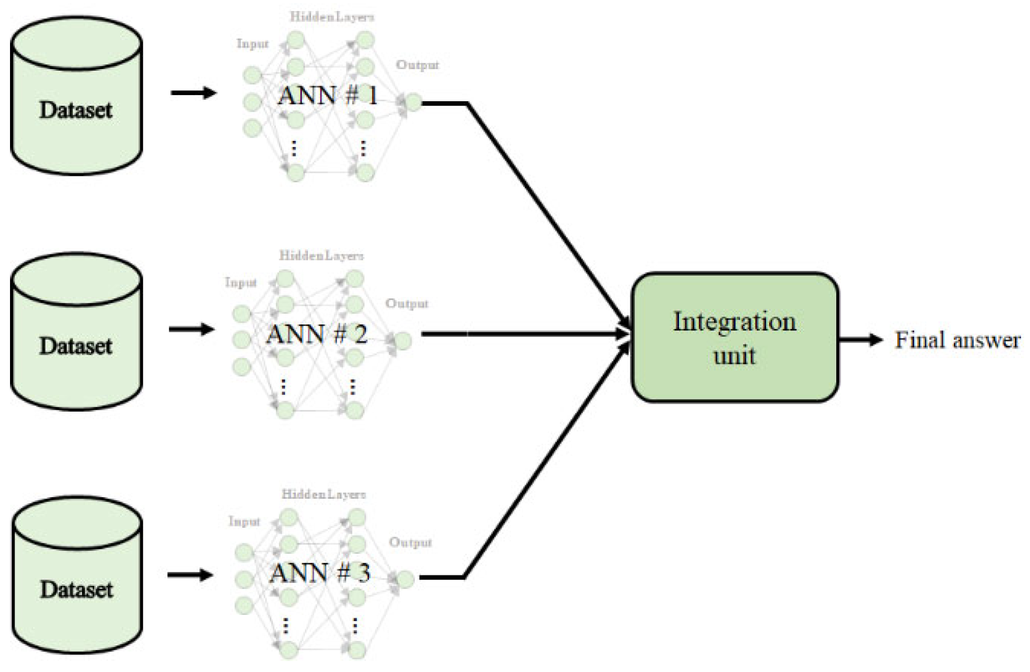
Figure 1.
Illustration of an artificial neural network.
Figure 1.
Illustration of an artificial neural network.
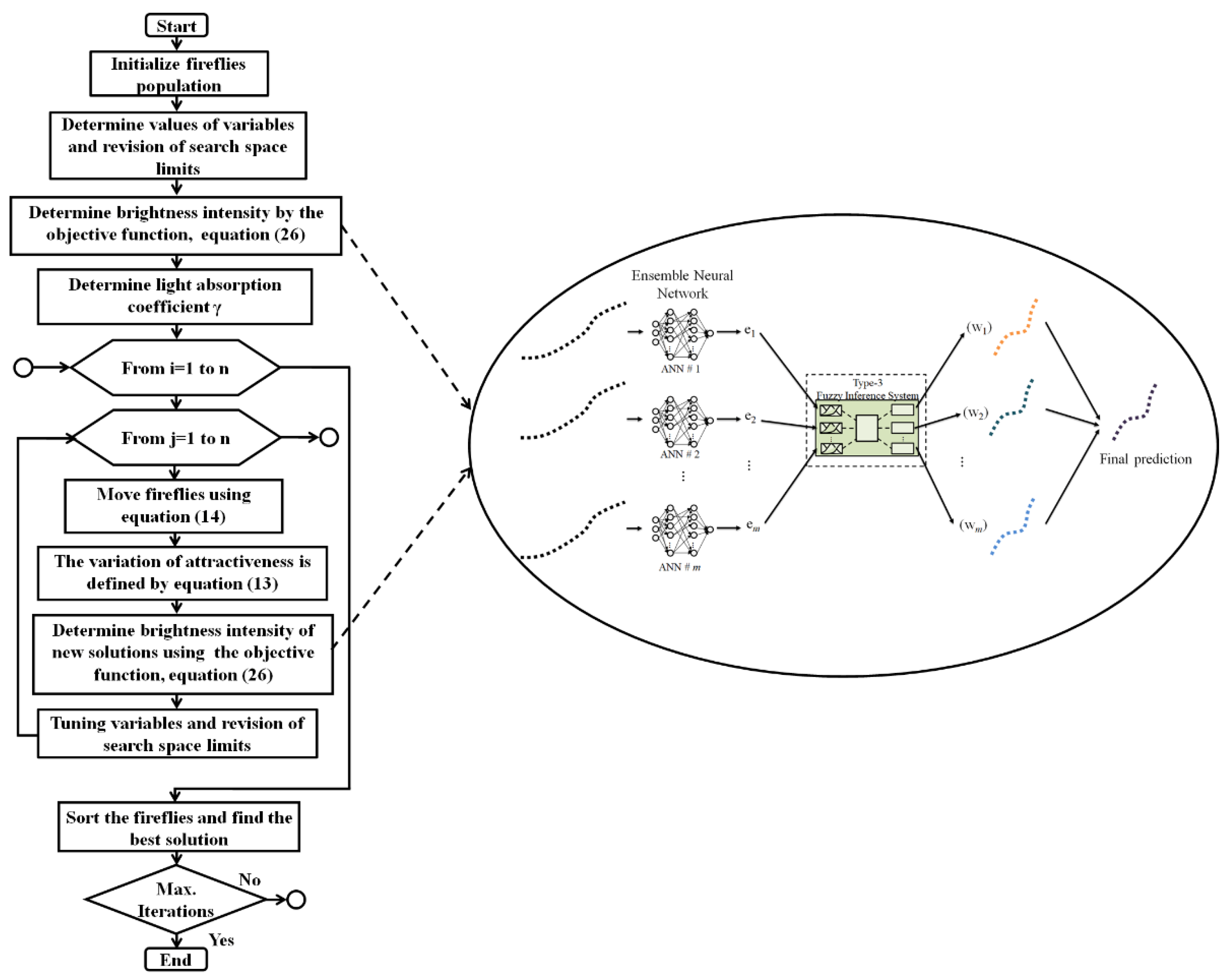
Figure 2.
Ensemble neural network.
Figure 2.
Ensemble neural network.
Figure 3.
Gaussian type-2 MF.
Figure 3.
Gaussian type-2 MF.
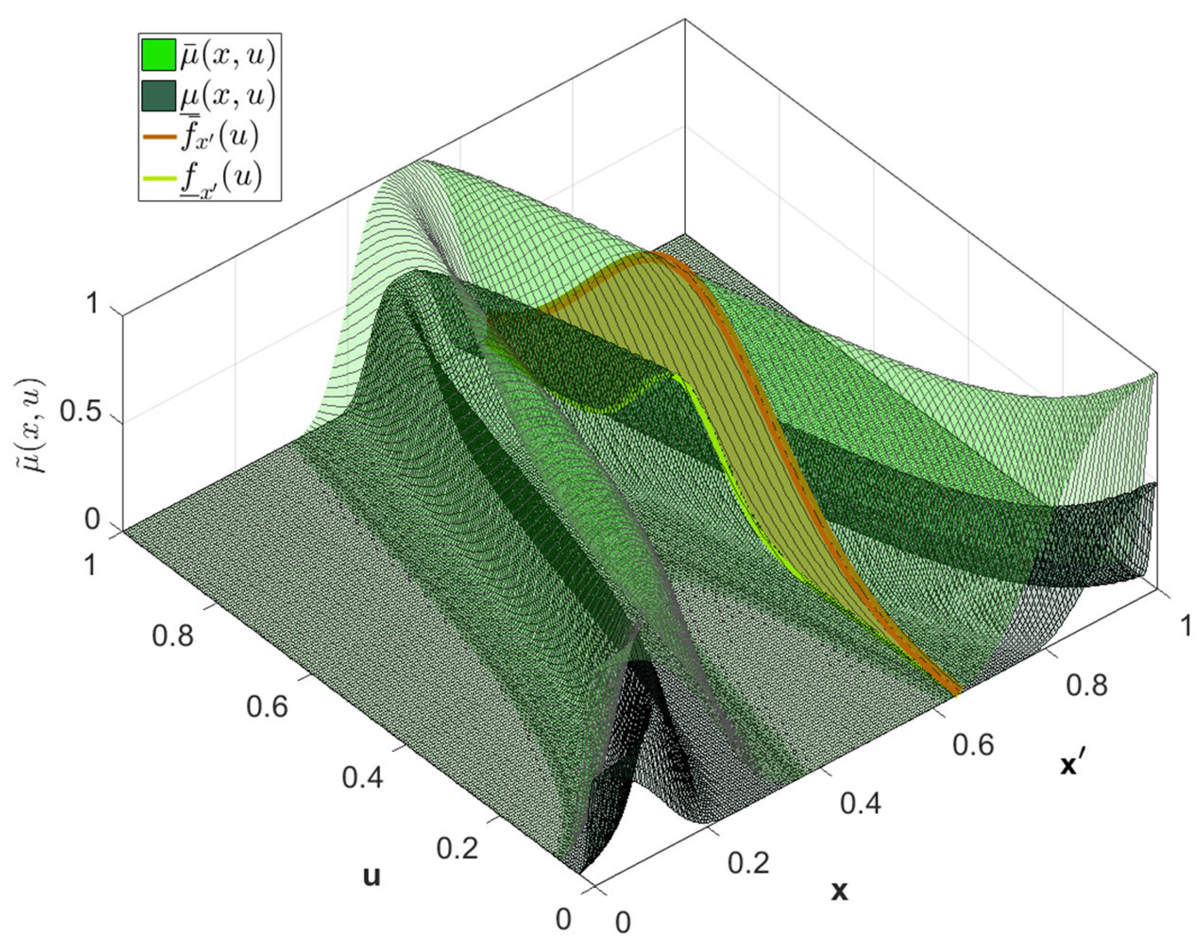
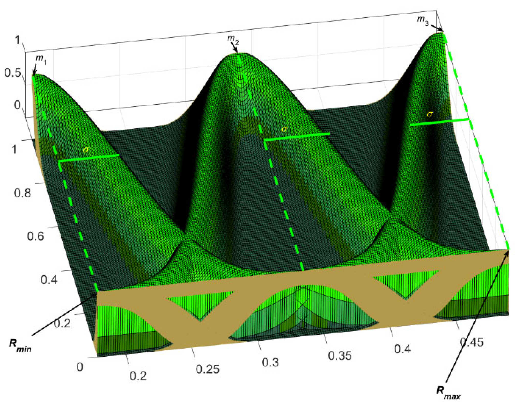
Figure 4.
Gaussian type-3 MF.
Figure 4.
Gaussian type-3 MF.
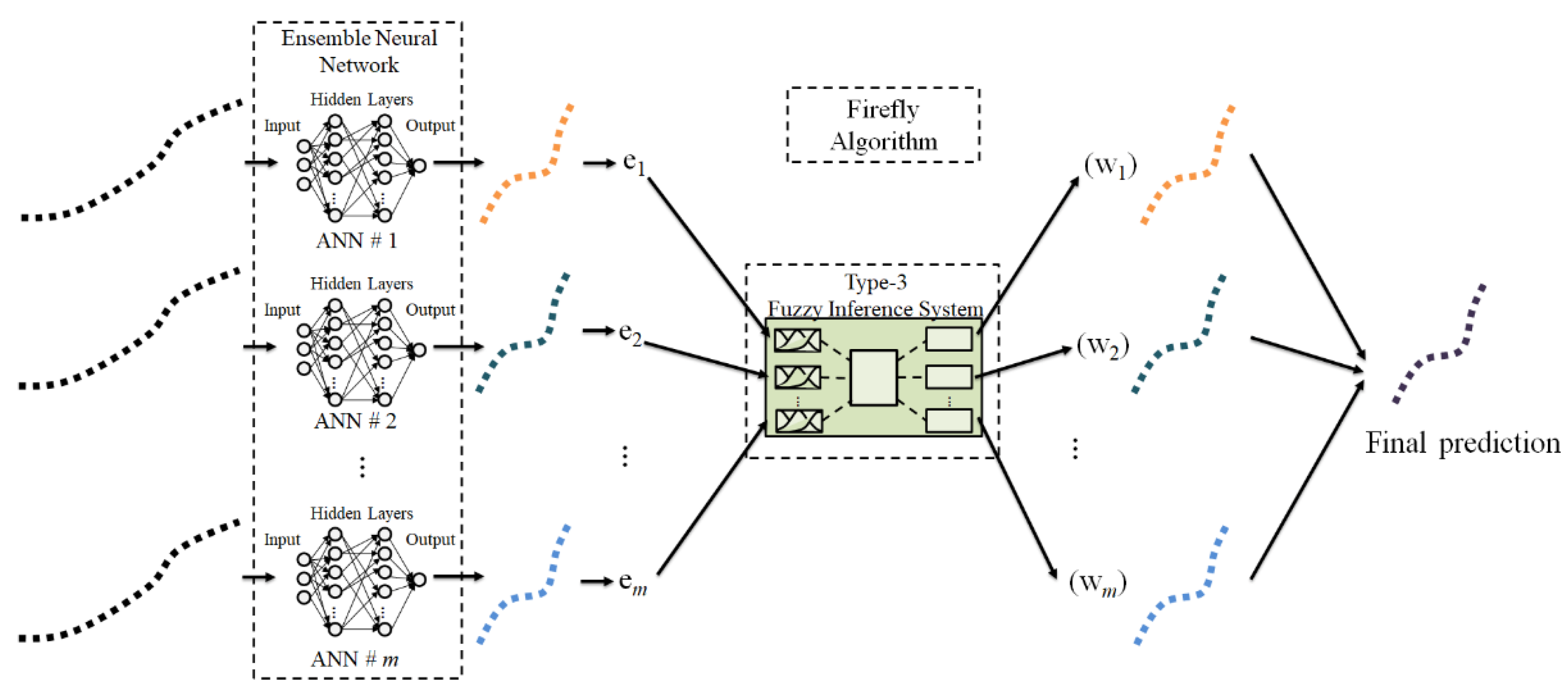
Figure 5.
The proposed ENNT3FL-FA.
Figure 5.
The proposed ENNT3FL-FA.
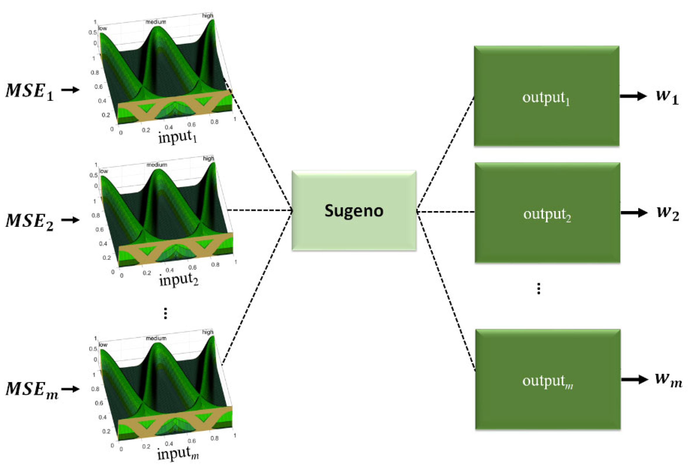
Figure 6.
Sugeno type-3 FIS model.
Figure 6.
Sugeno type-3 FIS model.
Figure 7.
Example of type-3 fuzzy input variable.
Figure 7.
Example of type-3 fuzzy input variable.
Figure 8.
Flowchart of the FA.
Figure 8.
Flowchart of the FA.
Figure 9.
First data period.
Figure 9.
First data period.
Figure 10.
Second data period.
Figure 10.
Second data period.
Figure 11.
Individual behavior and final prediction for Brazil: (a) module #1; (b) module #2; (c) module #3; (d) final prediction.
Figure 11.
Individual behavior and final prediction for Brazil: (a) module #1; (b) module #2; (c) module #3; (d) final prediction.
Figure 12.
Best future prediction (Brazil).
Figure 12.
Best future prediction (Brazil).
Figure 13.
Type-3 fuzzy input variables (Brazil): (a) fuzzy input #1; (b) fuzzy input #2; (c) fuzzy input #3.
Figure 13.
Type-3 fuzzy input variables (Brazil): (a) fuzzy input #1; (b) fuzzy input #2; (c) fuzzy input #3.
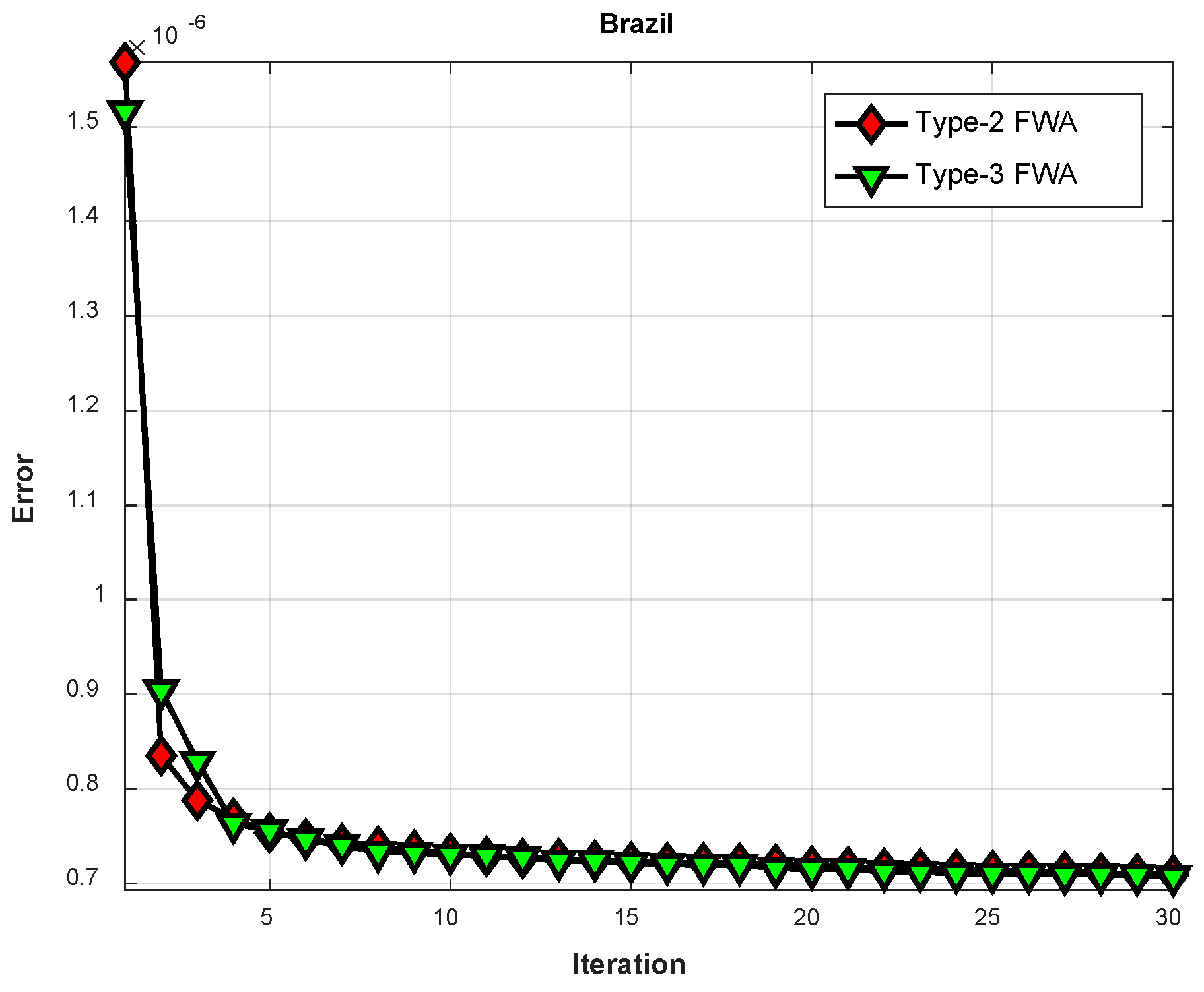
Figure 14.
Average convergence for Brazil.
Figure 14.
Average convergence for Brazil.
Figure 15.
Future prediction (Brazil).
Figure 15.
Future prediction (Brazil).
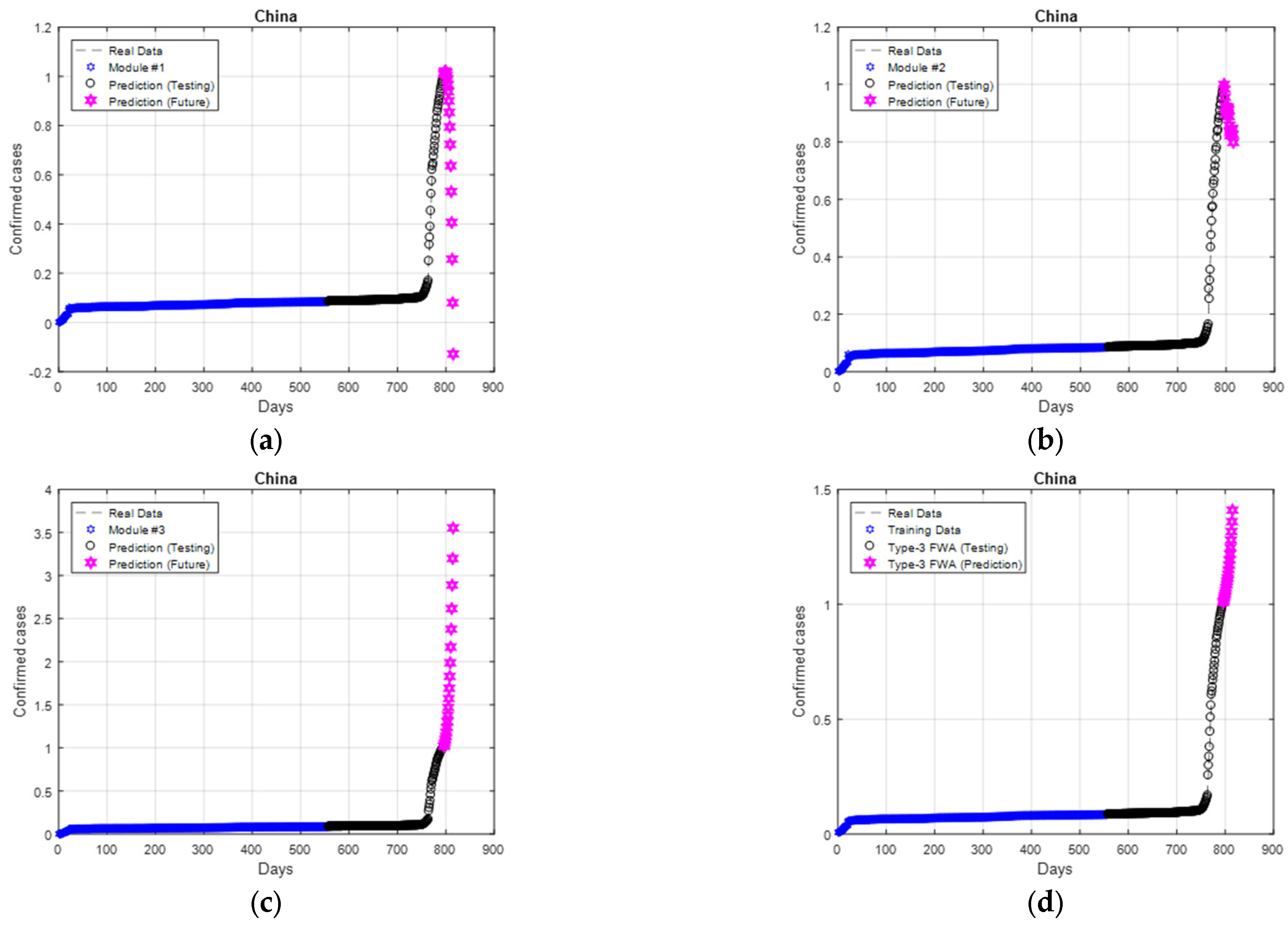
Figure 16.
Individual behavior and final prediction for China: (a) module #1; (b) module #2; (c) module #3; (d) final prediction.
Figure 16.
Individual behavior and final prediction for China: (a) module #1; (b) module #2; (c) module #3; (d) final prediction.
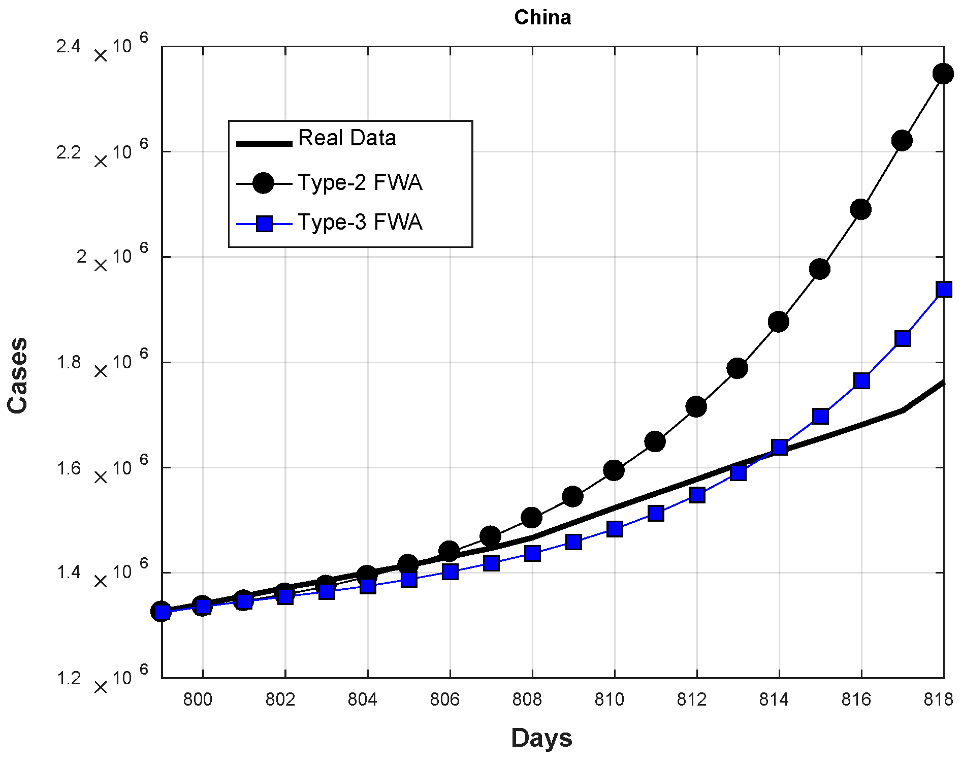
Figure 17.
Best future prediction (China).
Figure 17.
Best future prediction (China).
Figure 18.
Type-3 fuzzy input variables (China): (a) fuzzy input #1; (b) fuzzy input #2; (c) fuzzy input #3.
Figure 18.
Type-3 fuzzy input variables (China): (a) fuzzy input #1; (b) fuzzy input #2; (c) fuzzy input #3.
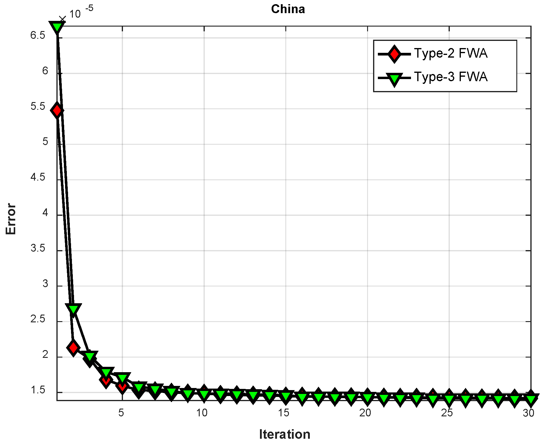
Figure 19.
Average convergence for China.
Figure 19.
Average convergence for China.
Figure 20.
Future prediction (China).
Figure 20.
Future prediction (China).
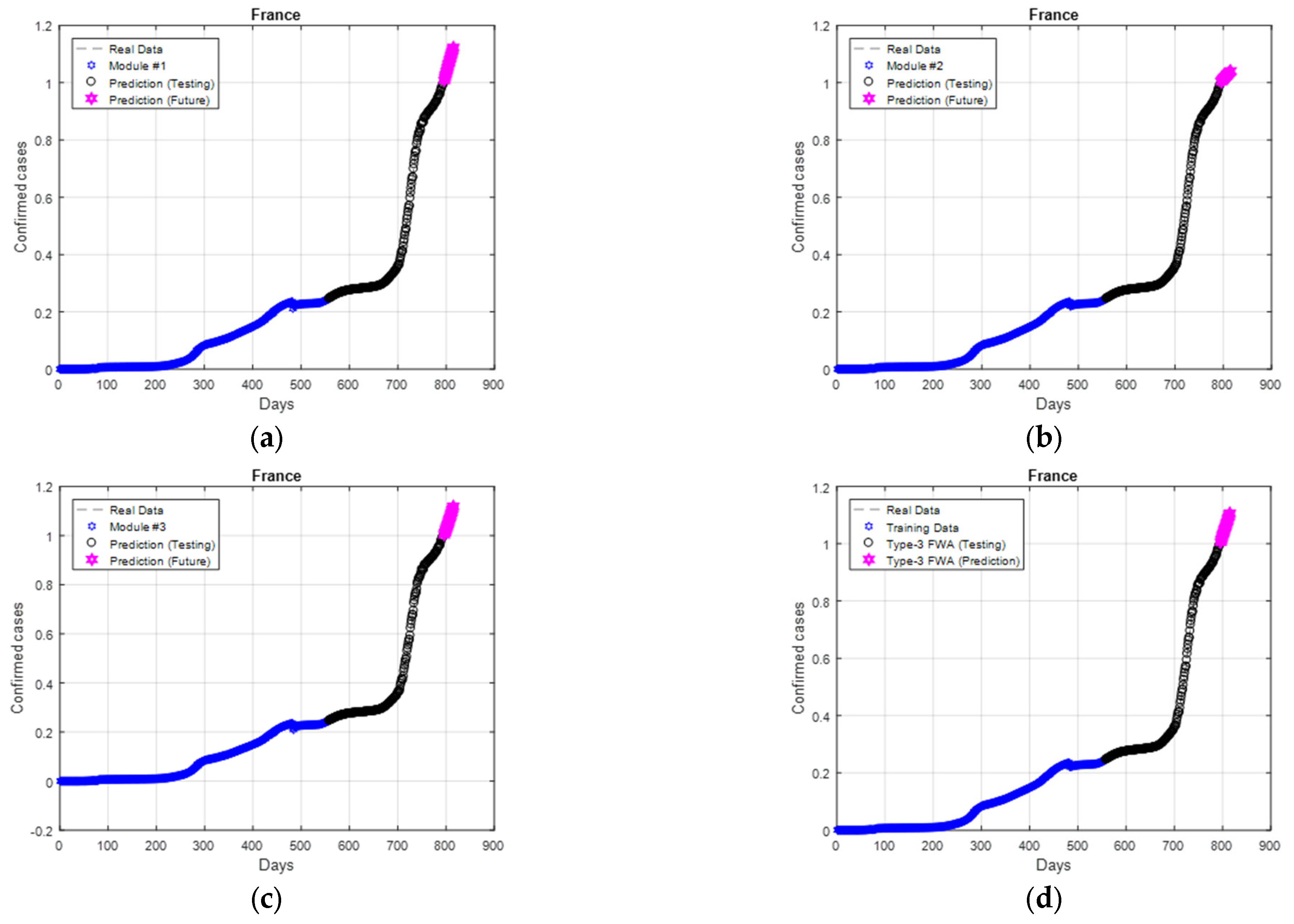
Figure 21.
Individual behavior and final prediction for France: (a) module #1; (b) module #2; (c) module #3; (d) final prediction.
Figure 21.
Individual behavior and final prediction for France: (a) module #1; (b) module #2; (c) module #3; (d) final prediction.
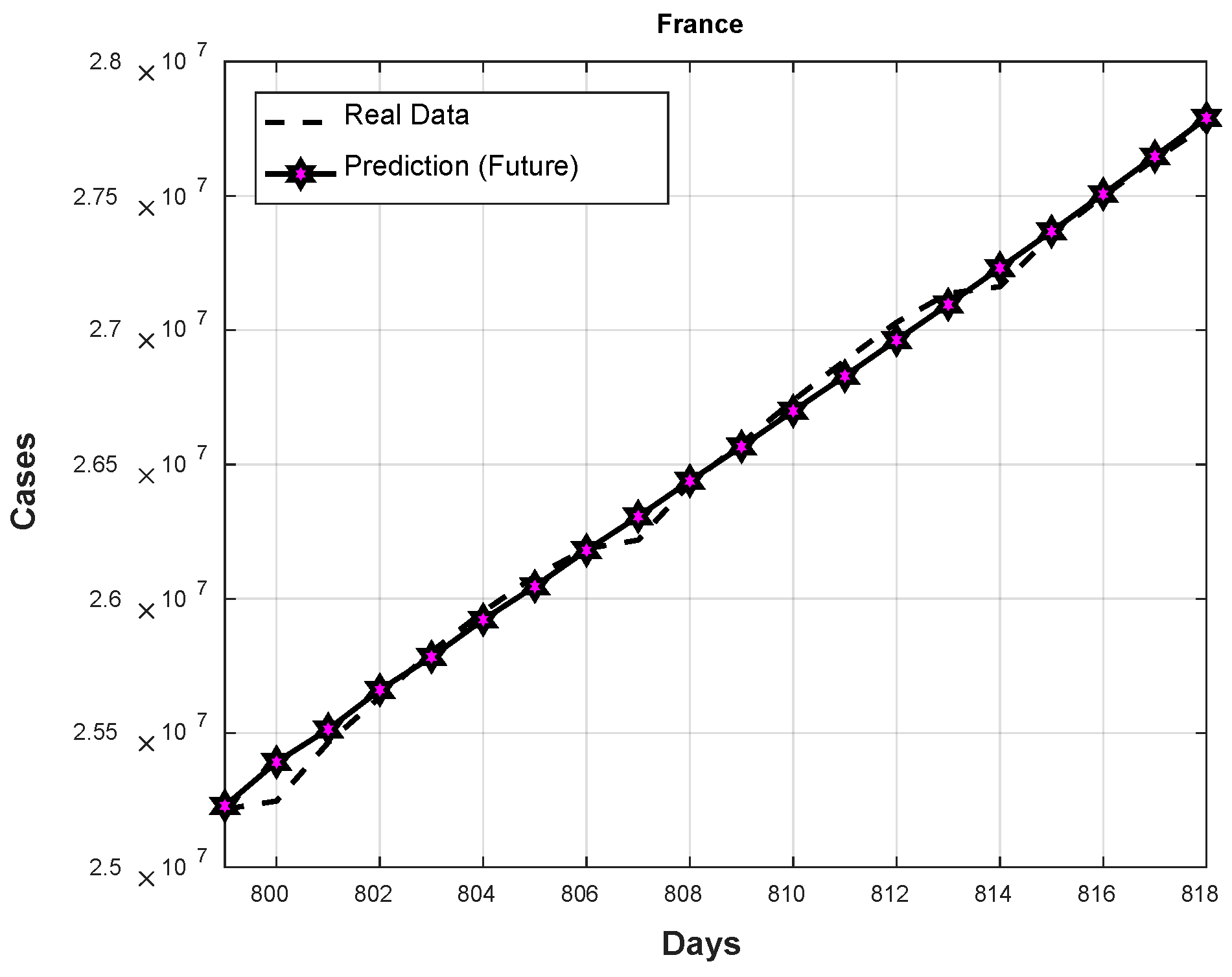
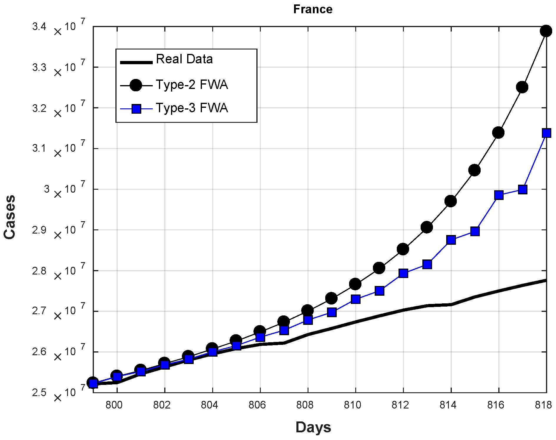
Figure 22.
Best future prediction (France).
Figure 22.
Best future prediction (France).
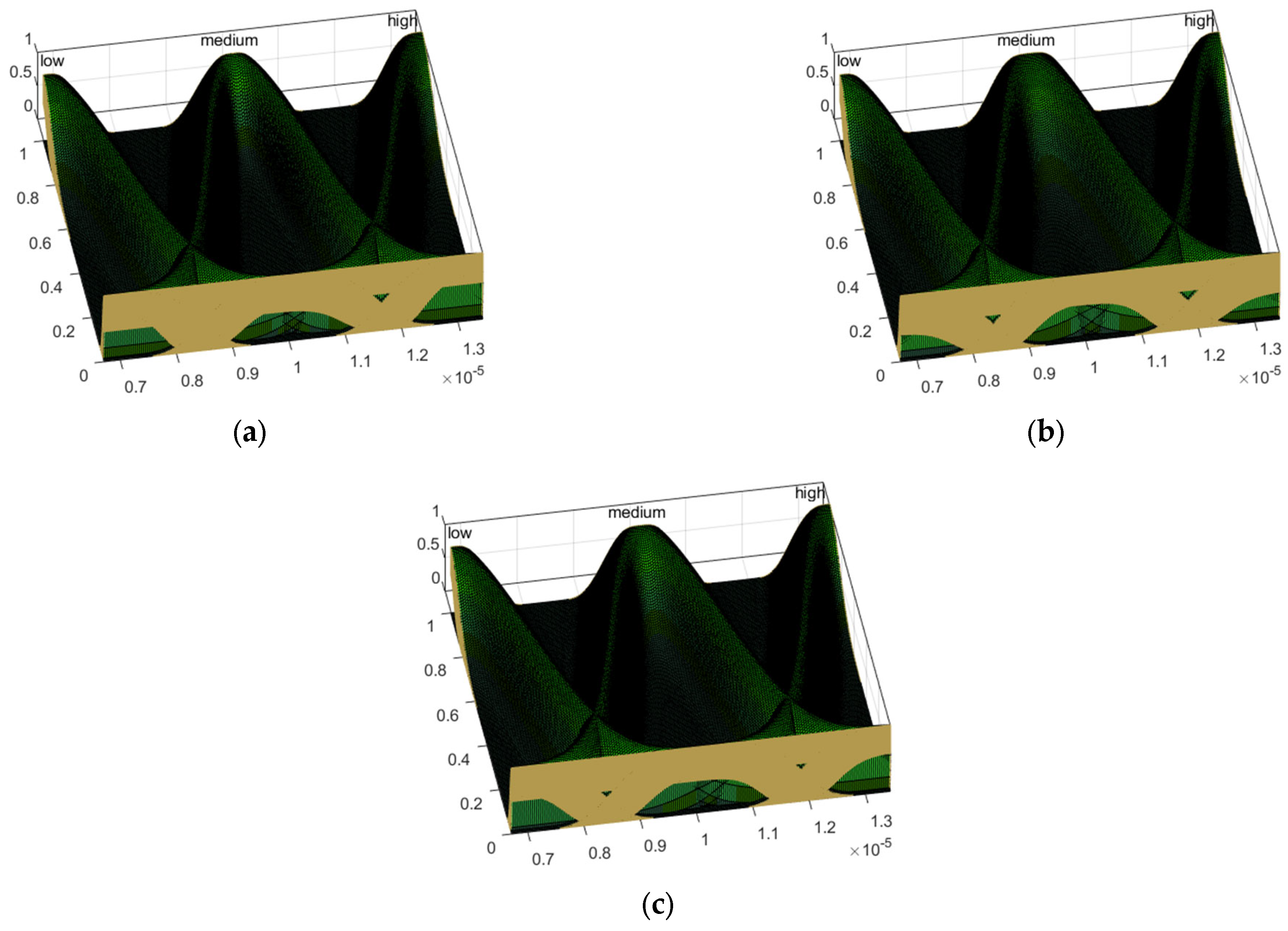
Figure 23.
Type-3 fuzzy input variables (France): (a) fuzzy input #1; (b) fuzzy input #2; (c) fuzzy input #3.
Figure 23.
Type-3 fuzzy input variables (France): (a) fuzzy input #1; (b) fuzzy input #2; (c) fuzzy input #3.
Figure 24.
Average convergence for France.
Figure 24.
Average convergence for France.
Figure 25.
Future prediction (France).
Figure 25.
Future prediction (France).
Figure 26.
First data period (testing prediction).
Figure 26.
First data period (testing prediction).
Figure 27.
First data period (future prediction).
Figure 27.
First data period (future prediction).
Figure 28.
Second data period (testing prediction).
Figure 28.
Second data period (testing prediction).
Figure 29.
Second data period (future prediction).
Figure 29.
Second data period (future prediction).
Table 1.
Fuzzy if-then rules for three inputs and outputs.
Table 1.
Fuzzy if-then rules for three inputs and outputs.
| Rule | Antecedents | Consequents |
|---|
| e1 | e2 | e3 | w1 | w2 | w3 |
|---|
| 1 | low | low | low | high | high | high |
| 2 | low | low | medium | high | high | medium |
| 3 | low | low | high | high | high | low |
| 4 | low | medium | low | high | medium | high |
| 5 | low | medium | medium | high | medium | medium |
| 6 | low | medium | high | high | medium | low |
| 7 | low | high | low | high | low | high |
| 8 | low | high | medium | high | low | medium |
| 9 | low | high | high | high | low | low |
| 10 | medium | low | low | medium | high | high |
| 11 | medium | low | medium | medium | high | medium |
| 12 | medium | low | high | medium | high | low |
| 13 | medium | medium | low | medium | medium | high |
| 14 | medium | medium | medium | medium | medium | medium |
| 15 | medium | medium | high | medium | medium | low |
| 16 | medium | high | low | medium | low | high |
| 17 | medium | high | medium | medium | low | medium |
| 18 | medium | high | high | medium | low | low |
| 19 | high | low | low | low | high | high |
| 20 | high | low | medium | low | high | medium |
| 21 | high | low | high | low | high | low |
| 22 | high | medium | low | low | medium | high |
| 23 | high | medium | medium | low | medium | medium |
| 24 | high | medium | high | low | medium | low |
| 25 | high | high | low | low | low | high |
| 26 | high | high | medium | low | low | medium |
| 27 | high | high | high | low | low | low |
Table 2.
Search space.
| | Parameters | Minimum | Maximum |
|---|
| ENN | Modules (m) | 2 | 5 |
| Hidden Layers (h) | 1 | 5 |
| Neurons for Each Hidden Layer | 1 | 50 |
| Goal Error | 0.00001 | 0.001 |
| Type-3 FIS | Lower Scale (λ) | 0.1 | 0.9 |
| Lower Lag (ℓ) | 0.1 | 0.9 |
| Constants | 0.1 | 0.9 |
Table 3.
Best architecture for Brazil.
Table 3.
Best architecture for Brazil.
| Type | Neurons | Individual
(MSE) | Testing
(MSE) | Future
(MSE) |
|---|
| Feedforward | 35, 25 | 9.58 × 10⁻⁷ | 7.70 × 10⁻⁶ | 1.84 × 10⁻⁶ |
| Fitnet | 28, 45 | 1.51 × 10⁻⁶ |
| Cascade | 26 | 7.49 × 10⁻⁷ |
Table 4.
First data period (testing prediction, Brazil).
Table 4.
First data period (testing prediction, Brazil).
| Type-2 FWA | Type-3 FWA |
|---|
| Best | Avg | Worst | Best | Avg | Worst |
|---|
| 6.88 × 10⁻⁷ | 7.09 × 10⁻⁷ | 7.38 × 10⁻⁷ | 6.90 × 10⁻⁷ | 7.07 × 10⁻⁷ | 7.90 × 10⁻⁷ |
Table 5.
First data period (future prediction, Brazil).
Table 5.
First data period (future prediction, Brazil).
| Type-2 FWA | Type-3 FWA |
|---|
| Best | Avg | Worst | Best | Avg | Worst |
|---|
| 3.04 × 10⁻⁶ | 1.97 × 10⁻² | 1.42 × 10⁻¹ | 1.84 × 10⁻⁶ | 2.46 × 10⁻² | 1.06 × 10⁻¹ |
Table 6.
Best architecture for China.
Table 6.
Best architecture for China.
| Type | Neurons | Individual
(MSE) | Testing
(MSE) | Future
(MSE) |
|---|
| Fitnet | 25 | 3.27 × 10⁻⁵ | 1.40 × 10⁻⁵ | 5.22 × 10⁻⁴ |
| Fitnet | 28 | 2.00 × 10⁻⁵ |
| Feedforward | 12 | 2.15 × 10⁻⁴ |
Table 7.
First data period (testing prediction, China).
Table 7.
First data period (testing prediction, China).
| Type-2 FWA | Type-3 FWA |
|---|
| Best | Avg | Worst | Best | Avg | Worst |
|---|
| 1.36 × 10⁻⁵ | 1.42 × 10⁻⁵ | 1.54 × 10⁻⁵ | 1.36 × 10⁻⁵ | 1.41 × 10⁻⁵ | 1.52 × 10⁻⁵ |
Table 8.
First data period (future prediction, China).
Table 8.
First data period (future prediction, China).
| Type-2 FWA | Type-3 FWA |
|---|
| Best | Avg | Worst | Best | Avg | Worst |
|---|
| 1.84 × 10⁻³ | 6.98 × 10⁻² | 2.96 × 10⁻¹ | 5.22 × 10⁻⁴ | 2.97 × 10⁻² | 1.61 × 10⁻¹ |
Table 9.
Best architecture for France.
Table 9.
Best architecture for France.
| Type | Neurons | Individual
(MSE) | Testing
(MSE) | Future
(MSE) |
|---|
| Fitnet | 26 | 6.71 × 10⁻⁶ | 6.14 × 10⁻⁶ | 4.13 × 10⁻⁶ |
| Cascade | 30 | 1.34 × 10⁻⁵ |
| Fitnet | 24 | 9.51 × 10⁻⁶ |
Table 10.
First data period (testing prediction, France).
Table 10.
First data period (testing prediction, France).
| Type-2 FWA | Type-3 FWA |
|---|
| Best | Avg | Worst | Best | Avg | Worst |
|---|
| 6.09 × 10⁻⁶ | 6.25 × 10⁻⁶ | 6.80 × 10⁻⁶ | 6.14 × 10⁻⁶ | 6.36 × 10⁻⁶ | 6.81 × 10⁻⁶ |
Table 11.
First data period (future prediction, France).
Table 11.
First data period (future prediction, France).
| Type-2 FWA | Type-3 FWA |
|---|
| Best | Avg | Worst | Best | Avg | Worst |
|---|
| 6.07 × 10⁻⁶ | 2.06 × 10⁻² | 1.94 × 10⁻¹ | 4.13 × 10⁻⁶ | 7.11 × 10⁻³ | 6.06 × 10⁻² |
Table 12.
First data period (testing prediction).
Table 12.
First data period (testing prediction).
| Country | Type-2 | Type-3 |
|---|
| Best | Avg | Worst | Best | Avg | Worst |
|---|
| Brazil | 6.88 × 10⁻⁷ | 7.09 × 10⁻⁷ | 7.38 × 10⁻⁷ | 6.90 × 10⁻⁷ | 7.07 × 10⁻⁷ | 7.90 × 10⁻⁷ |
| China | 1.36 × 10⁻⁵ | 1.42 × 10⁻⁵ | 1.54 × 10⁻⁵ | 1.36 × 10⁻⁵ | 1.41 × 10⁻⁵ | 1.52 × 10⁻⁵ |
| France | 6.09 × 10⁻⁶ | 6.25 × 10⁻⁶ | 6.80 × 10⁻⁶ | 6.14 × 10⁻⁶ | 6.36 × 10⁻⁶ | 6.81 × 10⁻⁶ |
| Germany | 1.56 × 10⁻⁶ | 1.94 × 10⁻⁶ | 2.30 × 10⁻⁶ | 1.61 × 10⁻⁶ | 2.02 × 10⁻⁶ | 2.84 × 10⁻⁶ |
| India | 4.90 × 10⁻⁸ | 5.08 × 10⁻⁸ | 5.83 × 10⁻⁸ | 4.90 × 10⁻⁸ | 5.14 × 10⁻⁸ | 5.84 × 10⁻⁸ |
| Iran | 2.13 × 10⁻⁷ | 2.23 × 10⁻⁷ | 2.33 × 10⁻⁷ | 2.14 × 10⁻⁷ | 2.28 × 10⁻⁷ | 2.46 × 10⁻⁷ |
| Italy | 2.56 × 10⁻⁶ | 2.58 × 10⁻⁶ | 2.61 × 10⁻⁶ | 2.55 × 10⁻⁶ | 2.59 × 10⁻⁶ | 2.64 × 10⁻⁶ |
| Mexico | 7.27 × 10⁻⁶ | 7.28 × 10⁻⁶ | 7.30 × 10⁻⁶ | 7.27 × 10⁻⁶ | 7.29 × 10⁻⁶ | 7.32 × 10⁻⁶ |
| Poland | 4.55 × 10⁻⁷ | 4.60 × 10⁻⁷ | 4.98 × 10⁻⁷ | 4.55 × 10⁻⁷ | 4.61 × 10⁻⁷ | 4.78 × 10⁻⁷ |
| Spain | 2.20 × 10⁻⁵ | 2.21 × 10⁻⁵ | 2.22 × 10⁻⁵ | 2.20 × 10⁻⁵ | 2.21 × 10⁻⁵ | 2.23 × 10⁻⁵ |
| United Kingdom | 8.42 × 10⁻⁶ | 8.55 × 10⁻⁶ | 8.80 × 10⁻⁶ | 8.36 × 10⁻⁶ | 8.54 × 10⁻⁶ | 8.79 × 10⁻⁶ |
| USA | 2.86 × 10⁻⁶ | 2.87 × 10⁻⁶ | 2.89 × 10⁻⁶ | 2.85 × 10⁻⁶ | 2.88 × 10⁻⁶ | 2.92 × 10⁻⁶ |
Table 13.
First data period (future days).
Table 13.
First data period (future days).
| Country | Type-2 | Type-3 |
|---|
| Best | Avg | Worst | Best | Avg | Worst |
|---|
| Brazil | 3.04 × 10⁻⁶ | 1.97 × 10⁻² | 1.42 × 10⁻¹ | 1.84 × 10⁻⁶ | 2.46 × 10⁻² | 1.06 × 10⁻¹ |
| China | 1.84 × 10⁻³ | 6.98 × 10⁻² | 2.96 × 10⁻¹ | 5.22 × 10⁻⁴ | 2.97 × 10⁻² | 1.61 × 10⁻¹ |
| France | 6.07 × 10⁻⁶ | 2.06 × 10⁻² | 1.94 × 10⁻¹ | 4.13 × 10⁻⁶ | 7.11 × 10⁻³ | 6.06 × 10⁻² |
| Germany | 8.02 × 10⁻⁴ | 8.55 × 10⁻² | 4.11 × 10⁻¹ | 4.09 × 10⁻⁵ | 3.02 × 10⁻² | 1.01 × 10⁻¹ |
| India | 1.56 × 10⁻⁷ | 8.89 × 10⁻³ | 1.54 × 10⁻¹ | 3.05 × 10⁻⁷ | 3.01 × 10⁻³ | 2.05 × 10⁻² |
| Iran | 1.12 × 10⁻⁵ | 1.78 × 10⁻² | 9.82 × 10⁻² | 7.56 × 10⁻⁷ | 1.43 × 10⁻² | 1.05 × 10⁻¹ |
| Italy | 7.57 × 10⁻⁶ | 4.54 × 10⁻² | 2.92 × 10⁻¹ | 1.24 × 10⁻⁵ | 1.76 × 10⁻² | 8.32 × 10⁻² |
| Mexico | 2.86 × 10⁻⁵ | 9.14 × 10⁻³ | 1.81 × 10⁻¹ | 1.48 × 10⁻⁵ | 1.49 × 10⁻³ | 3.00 × 10⁻² |
| Poland | 8.31 × 10⁻⁵ | 2.05 × 10⁻² | 4.28 × 10⁻¹ | 5.71 × 10⁻⁵ | 6.08 × 10⁻³ | 5.85 × 10⁻² |
| Spain | 5.82 × 10⁻⁴ | 9.17 × 10⁻⁴ | 1.54 × 10⁻³ | 5.56 × 10⁻⁴ | 8.37 × 10⁻⁴ | 1.54 × 10⁻³ |
| United Kingdom | 2.80 × 10⁻⁵ | 7.07 × 10⁻³ | 1.62 × 10⁻¹ | 2.69 × 10⁻⁴ | 1.26 × 10⁻² | 9.98 × 10⁻² |
| USA | 3.15 × 10⁻⁶ | 8.02 × 10⁻³ | 6.04 × 10⁻² | 6.26 × 10⁻⁷ | 5.32 × 10⁻³ | 9.49 × 10⁻² |
Table 14.
Second data period (testing prediction).
Table 14.
Second data period (testing prediction).
| Country | Type-2 | Type-3 |
|---|
| Best | Avg | Worst | Best | Avg | Worst |
|---|
| Brazil | 3.27 × 10⁻⁵ | 4.09 × 10⁻⁵ | 4.47 × 10⁻⁵ | 3.77 × 10⁻⁵ | 4.17 × 10⁻⁵ | 4.34 × 10⁻⁵ |
| China | 2.40 × 10⁻⁸ | 2.66 × 10⁻⁸ | 3.13 × 10⁻⁸ | 2.31 × 10⁻⁸ | 2.94 × 10⁻⁸ | 3.64 × 10⁻⁸ |
| France | 2.14 × 10⁻⁵ | 2.56 × 10⁻⁵ | 2.94 × 10⁻⁵ | 2.15 × 10⁻⁵ | 2.50 × 10⁻⁵ | 2.76 × 10⁻⁵ |
| Germany | 1.90 × 10⁻⁶ | 2.00 × 10⁻⁶ | 2.17 × 10⁻⁶ | 1.85 × 10⁻⁶ | 2.01 × 10⁻⁶ | 2.15 × 10⁻⁶ |
| India | 1.95 × 10⁻⁶ | 2.06 × 10⁻⁶ | 2.36 × 10⁻⁶ | 1.90 × 10⁻⁶ | 2.09 × 10⁻⁶ | 2.29 × 10⁻⁶ |
| Iran | 1.40 × 10⁻⁶ | 1.47 × 10⁻⁶ | 1.49 × 10⁻⁶ | 1.43 × 10⁻⁶ | 1.48 × 10⁻⁶ | 1.52 × 10⁻⁶ |
| Italy | 4.37 × 10⁻⁷ | 4.55 × 10⁻⁷ | 4.92 × 10⁻⁷ | 3.86 × 10⁻⁷ | 4.53 × 10⁻⁷ | 4.79 × 10⁻⁷ |
| Mexico | 8.13 × 10⁻⁶ | 8.55 × 10⁻⁶ | 9.11 × 10⁻⁶ | 8.19 × 10⁻⁶ | 8.53 × 10⁻⁶ | 9.02 × 10⁻⁶ |
| Poland | 6.21 × 10⁻⁶ | 6.76 × 10⁻⁶ | 6.99 × 10⁻⁶ | 6.12 × 10⁻⁶ | 6.75 × 10⁻⁶ | 6.98 × 10⁻⁶ |
| Spain | 2.42 × 10⁻⁶ | 2.59 × 10⁻⁶ | 2.64 × 10⁻⁶ | 2.44 × 10⁻⁶ | 2.60 × 10⁻⁶ | 2.64 × 10⁻⁶ |
| United Kingdom | 4.97 × 10⁻⁶ | 5.93 × 10⁻⁶ | 6.03 × 10⁻⁶ | 5.87 × 10⁻⁶ | 5.99 × 10⁻⁶ | 6.04 × 10⁻⁶ |
| USA | 1.50 × 10⁻⁶ | 1.52 × 10⁻⁶ | 1.54 × 10⁻⁶ | 1.50 × 10⁻⁶ | 1.52 × 10⁻⁶ | 1.54 × 10⁻⁶ |
Table 15.
Second data period (future days).
Table 15.
Second data period (future days).
| Country | Type-2 | Type-3 |
|---|
| Best | Avg | Worst | Best | Avg | Worst |
|---|
| Brazil | 8.58 × 10⁻⁴ | 9.30 × 10⁻² | 4.50 × 10⁻¹ | 9.21 × 10⁻⁴ | 6.70 × 10⁻² | 1.60 × 10⁻¹ |
| China | 1.76 × 10⁻⁷ | 2.89 × 10⁻⁵ | 2.74 × 10⁻⁴ | 3.53 × 10⁻⁷ | 2.43 × 10⁻⁴ | 5.68 × 10⁻³ |
| France | 2.42 × 10⁻⁵ | 1.33 × 10⁻³ | 5.23 × 10⁻³ | 9.87 × 10⁻⁶ | 1.95 × 10⁻³ | 1.01 × 10⁻² |
| Germany | 8.66 × 10⁻⁷ | 2.04 × 10⁻⁴ | 1.07 × 10⁻³ | 8.56 × 10⁻⁷ | 1.30 × 10⁻⁴ | 8.71 × 10⁻⁴ |
| India | 8.38 × 10⁻⁴ | 1.17 × 10⁻¹ | 5.58 × 10⁻¹ | 1.07 × 10⁻⁴ | 1.12 × 10⁻¹ | 3.97 × 10⁻¹ |
| Iran | 5.63 × 10⁻⁶ | 5.77 × 10⁻⁴ | 1.36 × 10⁻² | 6.40 × 10⁻⁶ | 6.91 × 10⁻⁴ | 1.30 × 10⁻² |
| Italy | 1.34 × 10⁻⁷ | 5.39 × 10⁻³ | 1.43 × 10⁻¹ | 2.20 × 10⁻⁷ | 2.46 × 10⁻⁴ | 2.63 × 10⁻³ |
| Mexico | 3.32 × 10⁻⁴ | 1.09 × 10⁻¹ | 6.09 × 10⁻¹ | 8.04 × 10⁻⁵ | 7.87 × 10⁻² | 4.52 × 10⁻¹ |
| Poland | 7.13 × 10⁻⁶ | 5.19 × 10⁻³ | 8.62 × 10⁻² | 8.39 × 10⁻⁶ | 2.98 × 10⁻³ | 3.88 × 10⁻² |
| Spain | 3.88 × 10⁻⁶ | 1.42 × 10⁻⁴ | 1.27 × 10⁻³ | 2.12 × 10⁻⁶ | 1.15 × 10⁻⁴ | 8.85 × 10⁻⁴ |
| United Kingdom | 2.61 × 10⁻⁵ | 3.62 × 10⁻⁴ | 2.09 × 10⁻³ | 2.70 × 10⁻⁵ | 1.97 × 10⁻⁴ | 7.12 × 10⁻⁴ |
| USA | 1.60 × 10⁻⁴ | 2.11 × 10⁻³ | 6.99 × 10⁻³ | 5.10 × 10⁻⁵ | 2.44 × 10⁻³ | 8.44 × 10⁻³ |
Table 16.
Mann–Whitney results (first data period, testing prediction).
Table 16.
Mann–Whitney results (first data period, testing prediction).
| Country | Median | p-Value |
|---|
| Type-2 | Type-3 |
|---|
| Brazil | 7.09 × 10⁻⁷ | 7.02 × 10⁻⁷ | 0.0989 |
| China | 1.41 × 10⁻⁵ | 1.40 × 10⁻⁵ | 0.5892 |
| France | 6.22 × 10⁻⁶ | 6.33 × 10⁻⁶ | 0.0094 |
| Germany | 1.94 × 10⁻⁶ | 2.03 × 10⁻⁶ | 0.2501 |
| India | 5.02 × 10⁻⁸ | 5.07 × 10⁻⁸ | 0.5058 |
| Iran | 2.23 × 10⁻⁷ | 2.27 × 10⁻⁷ | 0.0251 |
| Italy | 2.58 × 10⁻⁶ | 2.58 × 10⁻⁶ | 0.1119 |
| Mexico | 7.28 × 10⁻⁶ | 7.28 × 10⁻⁶ | 0.1494 |
| Poland | 4.58× 10⁻⁷ | 4.60 × 10⁻⁷ | 0.3478 |
| Spain | 2.21× 10⁻⁵ | 2.21 × 10⁻⁵ | 0.1236 |
| United Kingdom | 8.53 × 10⁻⁶ | 8.51 × 10⁻⁶ | 0.4295 |
| USA | 2.87 × 10⁻⁶ | 2.87 × 10⁻⁶ | 0.0785 |
Table 17.
Mann–Whitney results (first data period, future prediction).
Table 17.
Mann–Whitney results (first data period, future prediction).
| Country | Median | p-Value |
|---|
| Type-2 | Type-3 |
|---|
| Brazil | 1.60 × 10⁻³ | 1.05 × 10⁻² | 0.0257 |
| China | 5.21 × 10⁻² | 1.69 × 10⁻² | 0.0035 |
| France | 5.84 × 10⁻³ | 9.99 × 10⁻⁴ | 0.2983 |
| Germany | 5.78 × 10⁻² | 1.98 × 10⁻² | 0.0394 |
| India | 2.45 × 10⁻⁴ | 3.39 × 10⁻⁴ | 0.9522 |
| Iran | 5.42 × 10⁻³ | 3.18 × 10⁻⁴ | 0.0854 |
| Italy | 8.36 × 10⁻³ | 5.97 × 10⁻³ | 0.1902 |
| Mexico | 3.50 × 10⁻⁴ | 2.34 × 10⁻⁴ | 0.1164 |
| Poland | 9.38 × 10⁻⁴ | 1.03 × 10⁻³ | 0.7414 |
| Spain | 8.91 × 10⁻⁴ | 8.09 × 10⁻⁴ | 0.1707 |
| United Kingdom | 6.06 × 10⁻⁴ | 2.17 × 10⁻³ | 0.0048 |
| USA | 2.28 × 10⁻⁴ | 2.64 × 10⁻⁴ | 0.3789 |
Table 18.
Mann–Whitney results (second data period, testing prediction).
Table 18.
Mann–Whitney results (second data period, testing prediction).
| Country | Median | p-Value |
|---|
| Type-2 | Type-3 |
|---|
| Brazil | 4.09 × 10⁻⁵ | 4.21 × 10⁻⁵ | 0.2609 |
| China | 2.65 × 10⁻⁸ | 2.97 × 10⁻⁸ | 0.0001 |
| France | 2.59 × 10⁻⁵ | 2.51 × 10⁻⁵ | 0.1971 |
| Germany | 1.99 × 10⁻⁶ | 2.02 × 10⁻⁶ | 0.4110 |
| India | 2.05 × 10⁻⁶ | 2.07 × 10⁻⁶ | 0.1353 |
| Iran | 1.47 × 10⁻⁶ | 1.48× 10⁻⁶ | 0.0166 |
| Italy | 4.55 × 10⁻⁷ | 4.55 × 10⁻⁷ | 0.9920 |
| Mexico | 8.51 × 10⁻⁶ | 8.50 × 10⁻⁶ | 0.6818 |
| Poland | 6.83 × 10⁻⁶ | 6.82 × 10⁻⁶ | 0.8999 |
| Spain | 2.62 × 10⁻⁶ | 2.62 × 10⁻⁶ | 0.5069 |
| United Kingdom | 5.97 × 10⁻⁶ | 6.00 × 10⁻⁶ | 0.0071 |
| USA | 1.52 × 10⁻⁶ | 1.52 × 10⁻⁶ | 0.8067 |
Table 19.
Mann–Whitney results (second data period, future prediction).
Table 19.
Mann–Whitney results (second data period, future prediction).
| Country | Median | p-Value |
| Type-2 | Type-3 |
| Brazil | 5.72 × 10⁻² | 6.70 × 10⁻² | 0.9920 |
| China | 1.19 × 10⁻⁵ | 4.49 × 10⁻⁶ | 0.0989 |
| France | 9.72 × 10⁻⁴ | 1.58 × 10⁻³ | 0.3077 |
| Germany | 7.64 × 10⁻⁵ | 6.80 × 10⁻⁵ | 0.5687 |
| India | 2.23 × 10⁻² | 5.76 × 10⁻² | 0.7718 |
| Iran | 8.83 × 10⁻⁵ | 2.96 × 10⁻⁵ | 0.1010 |
| Italy | 1.09 × 10⁻⁴ | 4.67 × 10⁻⁵ | 0.1052 |
| Mexico | 6.84 × 10⁻² | 2.27 × 10⁻² | 0.1770 |
| Poland | 1.08 × 10⁻³ | 1.04 × 10⁻³ | 0.7263 |
| Spain | 4.11 × 10⁻⁵ | 4.49 × 10⁻⁵ | 0.4715 |
| United Kingdom | 2.64 × 10⁻⁴ | 1.60× 10⁻⁴ | 0.1096 |
| USA | 2.04 × 10⁻³ | 2.29× 10⁻³ | 0.3421 |


