Article

A Simultaneous Estimation of the Baseline Intensity and Parameters for Modulated Renewal Processes

1
The Institute of Statistical Mathematics, 10-3 Midori-Cho, Tachikawa, Tokyo 190-8562, Japan
2
Independent Researcher, 4-27-115 Sakuragaoka, Higashi-Yamato, Tokyo 207-0022, Japan
*
Author to whom correspondence should be addressed.
Axioms 2022, 11(7), 303; https://doi.org/10.3390/axioms11070303
Submission received: 13 January 2022 / Revised: 19 June 2022 / Accepted: 20 June 2022 / Published: 23 June 2022

Abstract

:
This paper proposes a semiparametric solution to estimate the intensity (hazard) function of modulated renewal processes: a nonparametric estimate for the baseline intensity function together with a parametric estimate of the model parameters of the covariate processes. Based on the martingale property associated with the conditional intensity, we construct a statistic from a residual analysis to estimate the baseline renewal intensity function, when the model parameters of the covariate processes are known. In addition, when the baseline intensity is obtained, the model parameters can be estimated using the usual maximum likelihood estimation. In practice, both the baseline intensity and model parameters are suggested to be estimated simultaneously via an expectation–maximization (E–M)-type iterative algorithm. A more important feature of the newly proposed algorithm is that, given n events in the observation dataset, its computation time is of order O ( n 2 ) , while the Nelson–Aalen–Breslow estimator takes a computation time of order O ( n 3 ) . For illustration, we apply the proposed estimation procedure to a set of data simulated from a modulated gamma renewal process and the aftershock sequence following the M s 8 Wenchuan earthquake, which occurred in Sichuan Province, China on 12 May 2008.

1. Introduction

The renewal process and its variants have been widely used in the studies of recurrent events [1,2] including episodes of illness, failures of a computer network system, wildfires in a particular forest, and major earthquakes on an active fault. Usually, a renewal process is taken as a starting point to model a sequence of such recurrent events, in which the lengths of the time intervals between each pair of neighboring events are identically and independently distributed. When the interevent times are also influenced by some external factors, the process then becomes a modulated renewal process (see e.g., [3]), which is formulated mathematically in the following way:
Consider a point process observed over time t [ 0 , T ] , and suppose that events occur at time 0 < T 1 < T 2 < < T n . Let N ( [ s , t ] ) ( s < t ) and H t denote the number of events occurring in the time interval [ s , t ] , and the history of the process at time t, respectively. We also write N ( t ) for N ( [ 0 , t ] ) and N ( t ) for N ( [ 0 , t ) ) . In general, a model for such a process is specified by its hazard function, also known as conditional intensity, defined as
λ ( t ) = lim Δ 0 E N ( [ t , t + Δ ) ) | H t Δ ,
i.e., the expectation of the number of events occurring in a unit time interval at t given the past history. For a modulated renewal process, the conditional intensity is often expressed in a multiplicative form:
λ ( t ) = μ ( t ) Z β ( t ) ,
where μ ( t ) = μ 0 ( t T N ( t ) ) , μ 0 ( x ) being the baseline hazard function and t T N ( t ) being the left-continuous backward recurrence time at t, and Z β ( t ) is a function of a time-varying covariate process with parameter vector β . In particular, when Z β ( t ) = 1 , N ( t ) reduces to an ordinary renewal process, where the time differences between two consecutive events, X i = T i T i 1 , for i = 1 , , n , are independently and identically distributed. In practice, μ 0 ( t ) can be interpreted as the internal property of the system, and Z β ( t ) explains the external influences to the intensity, or the responses of the system to the external environments. For example, when modeling the recurrence of a characteristic earthquake in a particular fault or region, μ 0 describes the intrinsic recurrence time, and Z β ( t ) represents the changes in tectonic environments, which may accelerate or decelerate the renewal of earthquake occurrences (e.g., [4]).
In past studies, the rich literature on survival analysis based on clinical data from a sample of patients or independent cluster samples (see, e.g., [3,5,6]) has deeply influenced studies on renewal processes and their variants. In survival analysis, the failure time X i for the ith individual ( i = 1 , ) are mutually independent with a modulated hazard function
h i ( x ) = h 0 ( x ) Z i , β ( x )
where h 0 is the baseline hazard function common to all individual, and Z i ( x ; β ) is the covariate function specific to the ith individual. Refs. [3,7,8] proposed a partial likelihood estimate for β in the absence of knowledge of the baseline intensity, i.e., the partial likelihood estimator β ^ is obtained by maximizing in β the partial likelihood
lik ( β ) = i = 1 n Z i , β ( X i ) j = 1 n 1 ( X j X i ) Z j , β ( X i )
where 1 ( A ) denotes the indicator function of the event A. Cox also suggested that the asymptotic inference about β proceeds as if the partial likelihood were an ordinary likelihood function.
For the estimation of the cumulative baseline hazard function, [9,10] considered a nonparametric estimate for the cumulative intensity from censored survival data to assess the fit of parametric models graphically for engineering applications. Under the framework of counting processes, [11,12] illustrated the use of this estimate in the studies of Markov chains and other event history models. The Nelson–Aalen estimator takes the form of
H ^ 0 ( x ) = i : X i < x n 1 j = 1 n 1 ( X j X i ) Z j , β ( X i )
for the integrated baseline hazard function
H 0 ( x ) = 0 x h 0 ( u ) d u .
Ref. [12] also discussed the small and large sample properties of the estimate using the martingale methods. Stimulated by [9,13] replaced β by the Cox’s estimate β ^ , i.e.,
H ^ 0 ( x ) = i : X i < x n 1 j = 1 n 1 ( X j X i ) Z j , β ^ ( X i )
The asymptotic properties were discussed by [5,14].
The connection between the renewal process and survival analysis is that instead of a series of absolute occurrence times, { T i : i = 1 , 2 , } , if we express the renewal process as a series of interevent intervals,
{ X i : X 1 = T 1 , X i = T i T i 1 , i = 2 , 3 , , } ,
the modulated renewal process is turned into survival data. This treatment enables us to apply the analyzing techniques from survival analysis to the modulated renewal processes. For the intensity estimation, for instance, [15] introduced a pseudo-martingale estimating equation based on such a time rearranging scheme. The word “pseudo-martingale” was used because the authors developed an estimating equation from the filtration with respect to the time intervals, but not the original occurrence times. For the modified renewal process, they in fact gave the same estimators as Cox’s partial likelihood estimator for β and the Nelson–Aalen–Breslow estimator for the cumulative baseline hazard function.
Unlike the tradition of avoiding a simultaneous estimation of the baseline intensity and model parameters in survival studies, we propose a pure martingale-based estimating procedure in the manner of an expectation–maximization (E–M)-type iterative algorithm by making use of the ideas of residual analysis of [16]. The ensuing sections are organized as follows. In Section 2, we first obtain a new estimating equation based on the martingale property of the conditional intensity to estimate the cumulative baseline intensity. Then, making use of the technique of partial integration, we also establish the maximum likelihood estimates for the model parameters. Section 3 briefly compares our estimate for the cumulative baseline intensity with the Nelson–Aalen and Breslow estimates. Section 4 illustrates the estimating performance of the proposed method by applying it to a simulated dataset from a modulated gamma renewal process and the aftershock data of the M 8.0 Wenchuan earthquake, which occurred on 12 May 2008, in Sichuan Province, China. Finally, a residual analysis based on the transformed time sequence is conducted to test the goodness-of-fit in Section 5.

2. Theory and Methodology

2.1. Estimation of Baseline Intensity

To estimate the baseline intensity μ 0 ( x ) , we make use of the residual analysis for the temporal or spatiotemporal point process developed by [16], which was stimulated from the residual analysis for spatial point processes (see [17]). Let N be a simple temporal point process in the interval [ 0 , T ] , admitting a conditional intensity λ ( t ) . According to the martingale property of the conditional intensity, for any predictable process (measurable with respect to the σ -algebra that is generated by sets of the form ( s , t ] × E , where E F s , and F s is the time filtration, ζ ( t ) 0 ,
E D ζ ( s ) d N ( s ) = E D ζ ( s ) λ ( s ) d s
where D is any regular (Lebesgue measurable) subset of [ 0 , T ] . Equation (8) holds since d M ( t ) = d N ( t ) λ ( t ) d t is a zero-mean martingale.
The first-order innovation with respect to a predictable function ζ ( t ) and a measurable set D [ 0 , T ] is defined by
V ( D , ζ , λ ) = D ζ ( s ) d N ( s ) D ζ ( s ) λ ( s ) d s
Because of (8), E [ V ( D , ζ , λ ) ] = 0 . The first-order residual is defined by replacing the true model in Equation (9) by the fitted model, i.e.,
R ( D , ζ ^ , λ ^ ) = D ζ ^ ( s ) d N ( s ) D ζ ^ ( s ) λ ^ ( s ) d s ,
where we use ζ ^ instead of ζ for the reason that ζ may include the estimated model parameters. If the fitted model is sufficiently close to the true model, then R ( D , ζ ^ , λ ^ ) 0 .
Ref. [16] also illustrated how to use the above techniques to reconstruct different components in the formation of a branching-type clustering model for describing the spatiotemporal clustering features of earthquake occurrences, which was called the epidemic-type aftershocks sequence (ETAS) model ([18,19]). In the following, we apply similar techniques to the multiplicative modulated processes in order to reconstruct the baseline intensity function.
Let N be a modulated renewal process with occurrence times T 1 , , T n and intensity function (2). Furthermore, let T 0 = 0 , T n + 1 = T , and X i = T i T i 1 , i = 1 , 2 , , n + 1 . For x > 0 , choose ζ x ( t ) as
ζ x ( t ) : = 1 ( t < T N ( t ) + x ) μ ( t ) λ ( t ) = 1 ( t < T N ( t ) + x ) Z β ( t ) , 0 t T , x 0 ,
and then (8) gives
E 0 T ζ ( s ) d N ( s ) = E 0 T 1 ( s < T N ( t ) + x ) μ ( s ) d s .
As the integral of the left hand side of (11) is actually equivalent to summing the integrand over the jump times T 1 , , T n of the process, we rewrite it as
0 T 1 ( s < T N ( t ) + x ) Z β ( s ) d N ( s ) = i = 1 n 1 ( X i < x ) Z β ( T i ) .
Additionally, we partition the integral of the right hand side of (11) into n + 1 parts:
0 T 1 ( s < T N ( t ) + x ) μ ( s ) d s = i = 1 n + 1 T i 1 T i 1 ( s < T i 1 + x ) μ ( s ) d s .
Now, dropping the expectation sign and inserting (12) and (13) into (11), we get an approximation
i = 1 n 1 ( T i T i 1 < x ) Z β ( T i ) i = 1 n + 1 1 ( X i < x ) U 0 ( X i ) + 1 ( X i x ) U 0 ( x )
where
U 0 ( x ) = 0 x μ 0 ( s ) d s
is the cumulative baseline intensity function. Rearranging (14), we obtain a recursive estimate of U 0 ( x ) :
U ^ 0 ( x ) = i = 1 n 1 ( X i < x ) / Z β ( T i ) i = 1 n + 1 1 ( X i < x ) U ^ 0 ( X i ) i = 1 n + 1 1 ( X i x ) ,
by setting U 0 ( 0 ) = 0 . It is easy to see that U ^ 0 ( x ) is a right-continuous function, if we change < and ≥ to ≤ and > in (14), respectively, we can obtain another estimate for U 0 ( x ) , which has the same values as U ^ 0 ( x ) at almost all the locations except that it is a left-continuous function. Thus, to eliminate the ambiguity of U ^ 0 ( x ) at each observed interevent time, we consider the following function,
U ˜ 0 ( x ) = 0 , x [ 0 , X ( 1 ) / 2 ] ω i ( x ) U ^ ( X ( i 1 ) ) + [ 1 ω i ( x ) ] U ^ ( X ( i ) ) , x ( X ( i 1 ) + X ( i ) ) / 2 , ( X ( i ) + X ( i + 1 ) ) / 2 , i = 1 , 2 , , n ω n ( x ) U ^ ( X ( n 1 ) ) + [ 1 ω n ( x ) ] U ^ ( X ( n ) ) , x [ ( X ( n ) + X ( n + 1 ) ) / 2 , ] ,
where { X ( i ) : i = 1 , 2 , , n + 1 } is the reordering of { X i : i = 1 , 2 , , n + 1 } in an ascending order, X ( 0 ) = 0 , and ω i ( x ) = [ 2 x ( X ( i 1 ) + X ( i ) ) ] / ( X ( i + 1 ) X ( i 1 ) ) represents the proportion of the segment cut by x from the left end of ( X ( i 1 ) + X ( i ) ) / 2 , ( X ( i ) + X ( i + 1 ) ) / 2 .

2.2. Estimation of Parameters in the External Process

The log-likelihood of a point process equipped with conditional intensity λ ( t ) is
log L = i = 1 n log λ ( T i ) 0 T λ ( s ) d s
(see [20]). When the baseline intensity is known, the maximum likelihood estimates of parameter β of model (2) is the maximizer of
log L = i = 1 n log μ 0 ( X i ) + log Z β ( T i ) i = 1 n + 1 0 X i μ 0 ( s ) Z β ( s + T i 1 ) d s .
The integral term of (17) can be rewritten by using partial integration
0 X i μ 0 ( s ) Z β ( s + T i 1 ) d s = 0 X i Z β ( s + T i 1 ) d U 0 ( s ) = Z β ( X i + T i 1 ) U 0 ( X i ) 0 X i U 0 ( s ) Z β ( s + T i 1 ) d s .
Recall that we can estimate U 0 by using (15) or (16) and that U ^ 0 is a stepwise function; (18) can be approximated by
0 X i μ 0 ( s ) Z β ( s + T i 1 ) d s Z β ( X i + T i 1 ) U ˜ 0 ( X i ) 0 X i U ^ 0 ( s ) Z β ( s + T i 1 ) d s .
Denote { X ( k ) : k = 1 , 2 , , n + 1 } in the ascending order of { X j : j = 1 , 2 , , n + 1 } . The integral term in the above equation can be rewritten as
0 X i U ^ 0 ( s ) Z β ( s + T i 1 ) d s = k : X ( k ) < X i U ^ ( X ( k ) ) Z β ( X ( k + 1 ) + T i 1 ) Z β ( X ( k ) + T i 1 ) .
In summary, the likelihood can be approximated by
log L i = 1 n { log μ 0 ( X i ) + log Z β ( T i ) Z β ( T i ) U ˜ 0 ( X i ) + k : X ( k ) < X i U ^ ( X ( k ) ) Z β ( X ( k + 1 ) + T i 1 ) Z β ( X ( k ) + T i 1 ) } .
As i = 1 n log μ 0 ( X i ) is independent of the model parameters, it can be omitted in the calculation of the maximum of the likelihood function. Similarly, the derivative of the likelihood function with respect to the model parameter can be approximated by
log L β i = 1 n { 1 Z β ( T i ) Z β ( T i ) β Z β ( T i ) β U ˜ 0 ( X i ) + k : X ( k ) < X i U ^ ( X ( k ) ) Z β ( X ( k + 1 ) + T i 1 ) β Z β ( X ( k ) + T i 1 ) β } .

2.3. Estimation Algorithm

As shown in Section 2.2, when μ 0 ( x ) is known, we can estimate the model parameter in Z β through a maximum likelihood estimation (MLE). Furthermore, when Z β is given, μ 0 ( x ) can be estimated by taking the derivative of a smoothed version of U ^ 0 ( x ) in Equation (15). However, in practice, both μ 0 ( x ) and Z β are unknown to us. What we have is a series of occurring times, T 1 , , T n , in a given observation period, say [ 0 , T ] , with or without other related information such as an external process or marks (such as sizes and location) of each event. To estimate μ 0 ( x ) and β simultaneously, we use the following iterative algorithm:
  • Step 1: Set 0 , μ ^ 0 ( ) ( s ) = n / T , or U ^ 0 ( ) ( s ) = n s / T , where n is the total number of event and [ 0 , T ] is the observing time window.
  • Step 2 (Maximization): Estimate β ( ) through an MLE, with U ^ 0 ( ) , i.e.,
    β ^ ( ) = arg max β log L = arg max β i = 1 n log Z β ( T i ) 0 X i μ 0 ( ) ( s ) Z β ( s + T i + 1 ) d s arg max β i = 1 n { log Z β ( T i ) Z β ( T i ) U ˜ 0 ( ) ( X i ) + k : X ( k ) < X i U ^ ( ) ( X ( k ) ) Z β ( X ( k + 1 ) + T i 1 ) Z β ( X ( k ) + T i 1 ) } ,
    where
    U ˜ 0 ( ) ( x ) = 0 , x 0 , X ( 1 ) 2 ω i ( x ) U ^ ( ) ( X ( i 1 ) ) + [ 1 ω i ( x ) ] U ^ 0 ( ) ( X ( i ) ) , x ( X ( i 1 ) + X ( i ) ) 2 , ( X ( i ) + X ( i + 1 ) ) 2 ω n ( x ) U ^ 0 ( ) ( X ( n 1 ) ) + [ 1 ω n ( x ) ] U ^ 0 ( ) ( X ( n ) ) , x X ( n ) + X ( n + 1 ) 2 , ,
    and ω i ( x ) = [ 2 x ( X ( i 1 ) + X ( i ) ) ] / ( X ( i + 1 ) X ( i 1 ) ) .
  • Step 3 (Expectation): Update
    U ^ 0 ( + 1 ) ( x ) = i = 1 n 1 ( X i < x ) / Z β ^ ( ) ( T i ) i = 1 n + 1 1 ( X i < x ) U ^ 0 ( + 1 ) ( X i ) i = 1 n + 1 1 ( X i x ) .
  • Step 4 (Rescaling): Let U ^ 0 ( + 1 ) ( x ) = U ^ 0 ( + 1 ) ( x ) / max U ^ 0 ( + 1 ) ( x ) .
  • Step 5: If max | U ^ 0 ( + 1 ) U ^ 0 ( ) | < ϵ , where ϵ is a small number, stop; otherwise, let + 1 , and go back to Step 2.
In Step 2, the term i = 1 n log μ 0 ( X i ) is dropped out in (20) because it is independent from β . Step 4 is introduced here because there is a free linear factor between function Z β and U 0 ( x ) , that is, if we divide Z β by a constant C and then multiply C by U 0 ( x ) , such a solution { Z β / C , C U 0 ( x ) } is equivalent to { Z β , U 0 ( x ) } .

3. Comparison with Existing Estimates

As mentioned in the introduction, it has been a tradition to construct statistical inferences of renewal processes in the manner of a survival analysis. Given the occurrence times of a renewal process, { T 1 , T 2 , , T n } , in an observation time window [ 0 , T ] , let T 0 = 0 and X i = T i T i 1 , i = 1 , , n , then the new sequence { X 1 , X 2 , , X n } forms up a survival process starting with n individuals. To study the differences between our estimate and those in survival processes, we compare our estimate of the cumulative baseline intensity with the Nelson–Aalen and Breslow estimates that were constructed based on partial likelihood (see [3,21]).
As mentioned in Section 1, after rearranging each interevent time as a survival sample that starts at time 0 and dies off after a period of the same length as the interevent time, the modulated renewal process is converted into a survival model with conditional intensity
λ ( x ) = μ 0 ( x ) i = 1 n 1 ( X i x ) Z β ( T i 1 + x ) .
If β is known, the cumulative baseline intensity U 0 ( x ) could be estimated by the Nelson–Aalen estimator
A ( x ) = 0 x d N ( s ) i = 1 n 1 ( X i s ) Z β ( T i 1 + s ) = X j x 1 i = 1 n 1 ( X i X j ) Z β ( T i 1 + X j ) .
If β is unknown and is replaced by its estimate β ^ , U 0 ( x ) could be estimated by the Breslow estimator
B ( x ) = 0 x d N ( s ) i = 1 n 1 ( X i s ) Z β ^ ( T i 1 + s ) = X j x 1 i = 1 n 1 ( X i X j ) Z β ^ ( T i 1 + X j )
The main difference between these two estimates and ours is the inclusion of the last interval of the event times in the estimation. In our study, we assume that the last interval is censored at time T, that is, the recurrence time of the ( n + 1 ) th observation is longer than X n + 1 , whereas in the partial likelihood estimation, there are no censored data in the last interval. In addition, concerns regarding the validity of using the Nelson–Aalen and Breslow estimators in modulated renewal processes were raised by [22,23], as the timescale reordering, from real time t to time interval x, might invalidate the conditioning argument underlying partial likelihood. As our estimate is martingale-based, its validity naturally holds according to the asymptotic properties related to martingales.

4. Applications

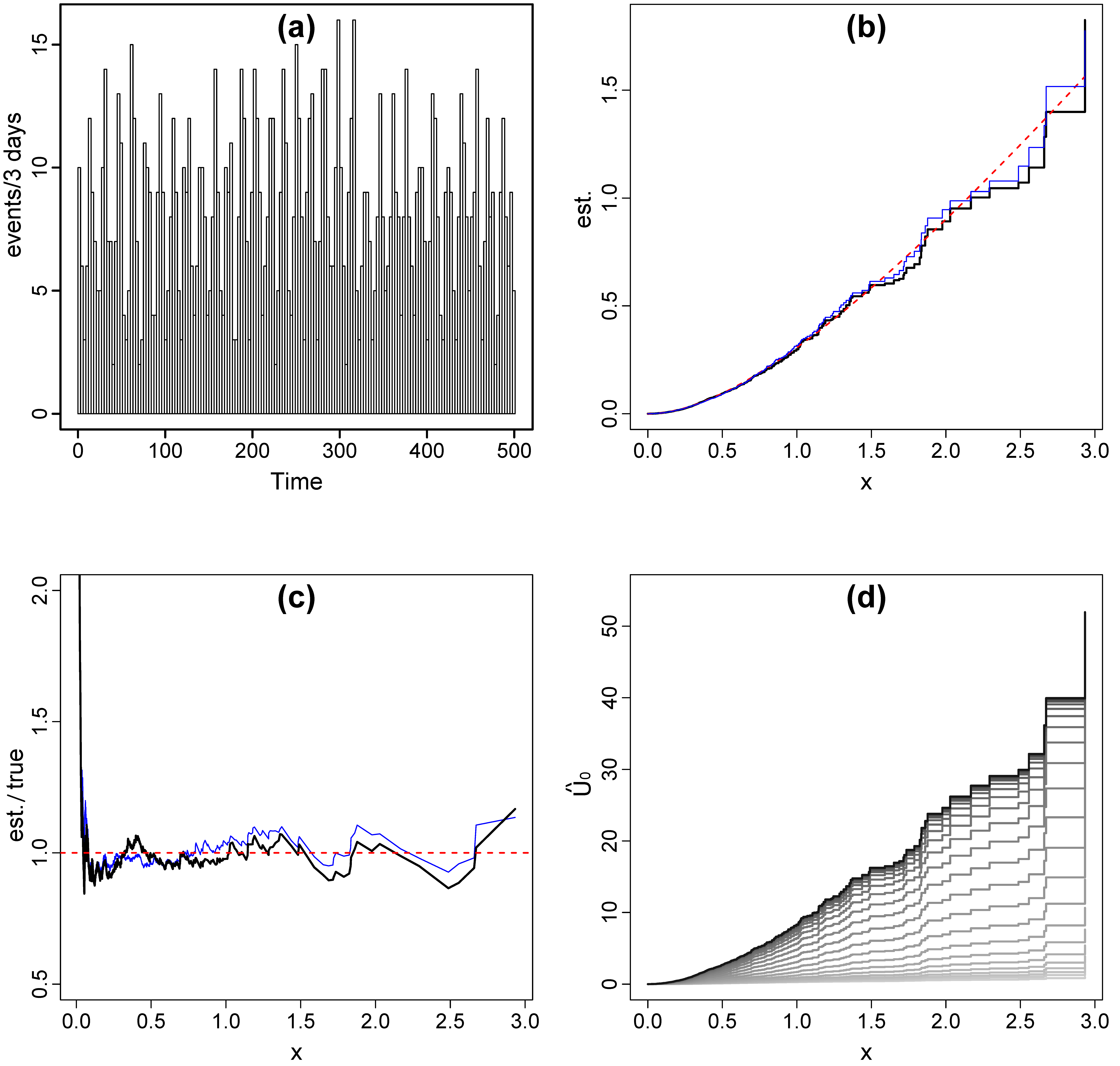
4.1. Simulation Study

In this example, we consider a modulated gamma renewal process with Z ( t ) = 2 + 30 sin 2 ( 0.2 t + 1.5 ) and μ 0 ( x ) = x e x / Γ ( 2 , x ) , where Γ denotes the incomplete gamma function. We simulated this process using the thinning algorithm given in Appendix A. Figure 1a displays the number of events occurring in a 3-day interval. We first assumed that the true Z β ( t ) is given, then applied (15) and (21) to the simulated data to get estimates of the cumulative baseline intensity, U ^ 0 ( x ) and A ( x ) , as shown in Figure 1b. Figure 1c gives the ratio of the estimates to the true U 0 ( x ) . From Figure 1b,c, we can see that the two estimates are almost identical to the true model, especially for small time intervals, and starts to diverge slightly when the size of the time interval increases.
To examine the convergence of our algorithm proposed in Section 2.3, we assumed that Z ( t ) = a + b sin 2 ( ω t + d ) , where ( a , b , ω , d ) is the parameter vector to be estimated. After some iterations, the final estimation converged to Z ^ ( t ) = 0.0799 + 1.0040 sin 2 ( 0.2000 t + 1.4466 ) . The convergence steps of U ^ 0 ( t ) are plotted in Figure 1d. To show the convergence steps more clearly in Figure 1d, we modified the rescaling step (Step 4) to U ^ 0 ( + 1 ) ( x ) = b ^ ( + 1 ) U ^ 0 ( + 1 ) ( x ) . The ratio of the finally estimated U ^ 0 ( x ) to the true U 0 ( x ) , U ^ 0 ( x ) / U 0 ( x ) , is similar to that in Figure 1c, but fluctuates around a different constant 28, which when multiplied with Z ^ ( t ) , yields a good estimate to the real values of parameters.

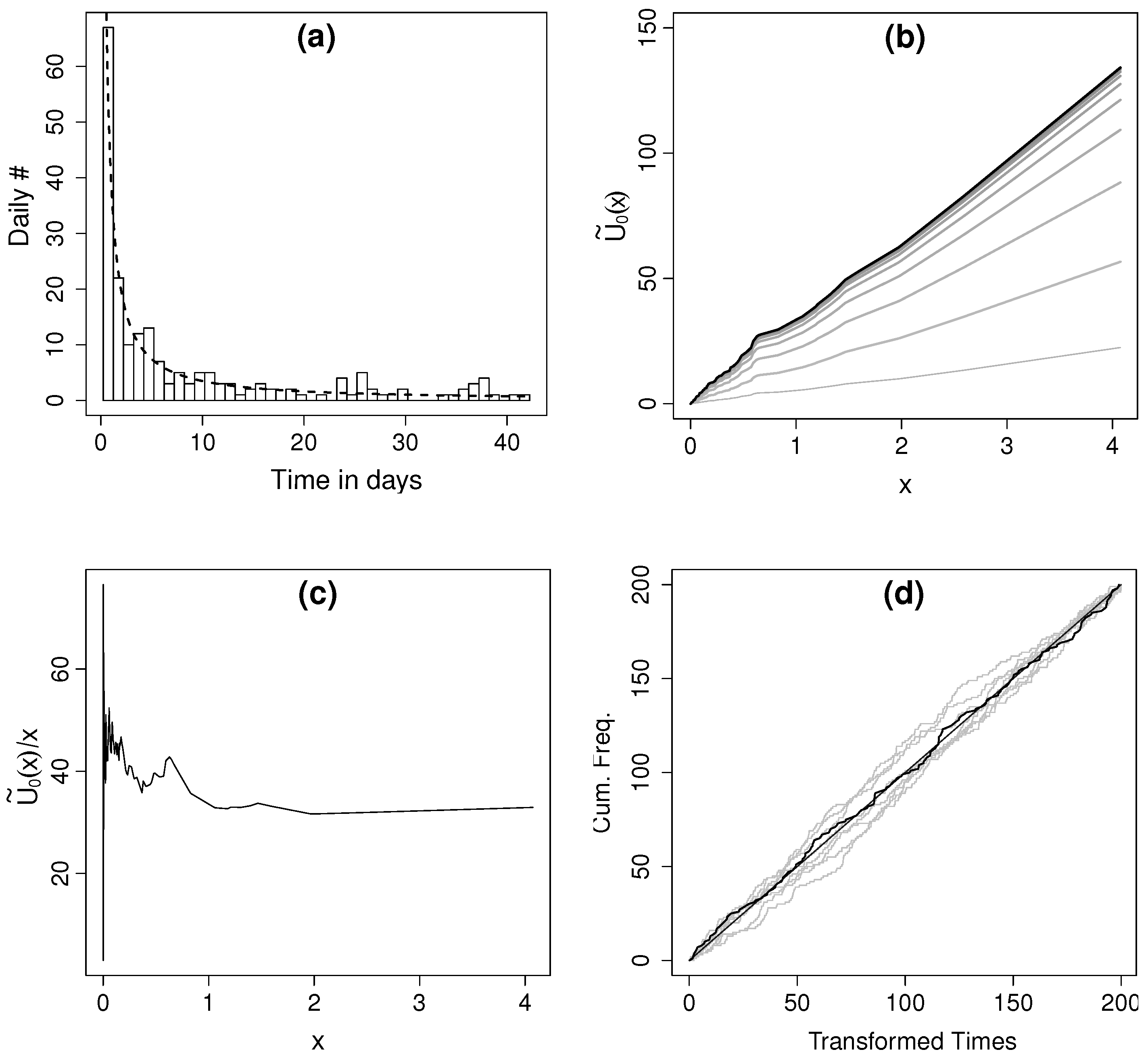
4.2. Real Data: Wenchuan Earthquake

In our second example, we applied our method to the aftershock data of the 2008 Wenchuan earthquake. This mainshock was measured at M s 8.0 and M w 7.9 and occurred at 14:28:01 CST (06:28:01 UTC) on Monday, 12 May 2008 in the Sichuan province of China, killing about 68,000 people. We selected the aftershocks of M s 4.0 for the analysis. In addition, as aftershocks immediately after a large mainshock are usually missing due to detection and recording problems (see, e.g., [24]), we neglected the event occurring within 0.225 days (about 5.4 h) after the occurrence of the mainshocks (see also [25]. Figure 2a gives the daily occurrence numbers of earthquakes.
In seismology, the Omori–Utsu formula ([26]; see [27], for a review) is a generally accepted empirical law for describing how the frequency of aftershocks decays with time. It asserts that the occurrence rate of aftershocks can be written as an inverse power law of time, i.e.,
n ( t ) = ν ( t + c ) p
where t is the time since the occurrence of the mainshock, ν is the amplitude, c is a “time-offset” parameter, and p modifies the decay rate of the aftershocks. All parameters are positive. In Figure 2a, the dashed line represents the results from fitting the Omori–Utsu formula, with ν ^ = 46.21 , c ^ = 0.1449 day, and p ^ = 1.1160 .
It is interesting to know whether the Omori-Utsu formula can describe the aftershock activity sufficiently; that is, if we regard the inverse power decay as the external modulation from the mainshock, whether the baseline hazard function is temporally constant. If so, the interevent time between the consecutive aftershocks behaves like a Poisson process, after the excitation effect from the mainshock is removed. We applied a modulated renewal model to the data, where the covariate process Z β ( t ) = ν 1 / ( t + c 1 ) p 1 was chosen to follow the Omori–Utsu formula.
The final estimates of the parameters in the fitted modulated renewal model were ν 1 ^ = 1.0010 , c 1 ^ = 0.0743 day, and p 1 ^ = 0.8270 . Figure 2b shows the convergence steps of U ^ 0 ( x ) . in Figure 2c, which gives the ratio of U ^ 0 ( x ) to the cumulative conditional intensity of a Poisson process of unit rate, i.e., U 0 Poisson ( x ) = x , we can see that the estimated baseline intensity has higher values at small time intervals and decreases to a constant when the time interval is large. This implies that, even if the triggering effect of the mainshock is modeled by the Omori–Utsu formula as the external modulating process and is eliminated by using the proposed technique, the interevent times between consecutive events do not always follow a Poisson process. For longer time intervals, the constant rate of the baseline intensity indicates that the larger interevent times are exponentially distributed. However, for the shorter time intervals, U 0 ( x ) / x is much larger than at longer time intervals, indicating that, beyond the clustering effect excited by the mainshock, there are further clusters occurring immediately after some of the aftershocks. In other words, the aftershock sequence from the Wenchuan earthquake shows a multistage triggering effect: not only the mainshock, but also the aftershocks can trigger their own aftershocks.

5. Transformed Time Analysis

When a model comparison is not presented, the technique of time-sequence transformation is a naive method to test goodness-of-fit. Notice that the following transformation of the original occurrence times of events,
T i τ i = 0 T i λ ( s ) d s
forms up a sequence { τ i : i = 1 , 2 , , n } . If the model is true, then { τ i : i = 1 , 2 , , n } should follow a standard Poisson process with unit rate (see, e.g., [18]). Thus, graphically, the plot of the cumulative frequencies of a fitted model against the transformed times would be close to a straight line if it fits the data well. For our study, the transformed time sequence for modulated renewal processes could be calculated based on Equation (19), i.e.,
τ 0 = 0 ; τ i + 1 τ i + U ˜ 0 ( X i ) Z β ^ ( T i ) 0 X i U ^ 0 ( s ) Z β ^ ( s + T i 1 ) d s = τ i + U ˜ 0 ( X i ) Z β ^ ( T i ) k : X ( k ) < X i U ^ ( X k ) Z β ^ ( X ( k + 1 ) + T i 1 ) Z β ^ ( X ( k ) + T i 1 ) .
Applying the above analysis to the Wenchuan aftershocks, the cumulative number of events against the transformed time sequence for the Wenchuan aftershocks are plotted in Figure 2d. The closeness between the curve of cumulative frequencies and the straight line of the unit slope shows the goodness-of-fit of the fitted-Omori–Utsu-formula modulated renewal process for the aftershock data. To understand the variation of the transformed times caused by randomness, we also simulated 10 realizations of a Poisson process with the same number of events as the Wenchuan aftershocks and rescaled their occurrence times in the interval [ 0 , n ] (see [28], for justification of 0 T λ ^ ( u ) d u = n ). The curve of the cumulative number of the transformed time sequence lies among the simulated curves, again indicating the goodness-of-fit of the fitted-Omori–Utsu-formula modulated renewal process.

6. Discussion

From (21) and (22), we can see that, for each x, the computational complexity of the Nelson–Aalen and Brewslow estimators are O ( n 2 ) , since these estimators have two layers of summations over the events in the processes. Considering that A ( x ) or B ( x ) are both stepwise constant functions, which change their values at nodes of n interevent times, the total computational complexity for estimating the entire A ( x ) or B ( x ) is O ( n 3 ) . From (15), the calculation of U ^ 0 ( x ) takes a computation time of the order O ( n ) at one location, and O ( n 2 ) at all locations. This is a great improvement from the Nelson–Aalen–Brewslow estimators and the method proposed by [15].
Another point is that we used the true likelihood function for estimating the model parameters in the modulating covariate processes instead of Cox’s maximizing partial likelihood estimator. In our procedure, once U ^ 0 ( x ) in (20) is obtained, the computation time of log L in (20) is also of the order of O ( n 2 ) , the same as the partial likelihood in Cox’s estimator in (4). In other words, the proposed algorithm does not increase the computational complexity in the parametric part.

7. Conclusions

This study presented a semiparametric method for simultaneously estimating the baseline hazard function and the parameters of a modulated renewal process. The core of this approach was an E–M-type iterative algorithm. The E step was the estimation of the integrated baseline hazard intensity obtained through constructing a zero-mean martingale, by assuming that the parameters of the external modulating effects were known. The M step was the MLE of the parameters in the external process, assuming the integrated baseline intensity was known. Compared to the Nelson–Aalen–Breslow estimator, the computation time of this algorithm was of the order of O ( n 2 ) for a dataset consisting of n events, while the Nelson–Aalen–Breslow estimator took a time of order O ( n 3 ) . The power of such a semiparametric method was illustrated through two examples: a simulated periodically modulated gamma renewal process and the aftershock sequences of the M s 8.0 Wenchuan earthquake, which occurred on 21 May 2008 in Sichuan Province, China. We also used the transformed time analysis to show the goodness-of-fit of our procedure to the Wenchuan earthquake.

Author Contributions

Conceptualization, J.Z.; methodology, H.-Y.S.; software and formal analysis, H.-Y.S. both authors have written, edited, and finalized the manuscript. All authors have read and agreed to the published version of the manuscript.

Funding

H.-Y. Siew was supported by the Global COE program of Meiji University for this study. Jiancang Zhuang is partially supported by JSPS Kakenhi Grant No. 19H04073. Helpful comments from two anonymous referees are gratefully acknowledged.

Institutional Review Board Statement

Not applicable.

Informed Consent Statement

Not applicable.

Data Availability Statement

Not applicable.

Conflicts of Interest

The authors declare no conflict of interest.

Appendix A. Algorithm for Simulating a Modulated Renewal Process

A modulated renewal process can be simulated based on the following thinning algorithm, which was designed according to Daley and Vere-Jones (2003, Algorithm 7.5.IV, Chapter 7):
Suppose that the process, which is equipped with a conditional intensity λ ( t ) = μ 0 ( t t N ( t ) ) Z ( t ) , has been simulated up to time t, with a record of { T 1 , T 2 , , T k } .
  • Step 1. Find three positive numbers D, M 1 , and M 2 such that M 1 μ 0 ( s T k ) and M 2 Z ( s ) for s ( t , t + D ) .
  • Step 2. Starting from t, generate the next event according to a Poisson process with rate M 1 M 2 . Suppose that its occurrence time is t , that is to say, t t has an exponential distribution with a rate of M 1 M 2 .
  • Step 3. Stop the simulation if t is greater than the termination time.
  • Step 4. If t > t + D , then let t = t + D and return to step 1.
  • Step 5. Generate an r. v. U U [ 0 , 1 ] . If U < μ 0 ( t T k ) M 1 Z ( t ) M 2 , accept t , i.e., set T k + 1 = t and k = k + 1 ; otherwise, let t = t and return to step 1.

References

  1. Cox, D.R. Renewal Theory; Methuen: London, UK, 1962. [Google Scholar]
  2. Cox, D.R.; Lewis, P.A.W. The Statistical Analysis of Series of Events; Methuen: London, UK, 1966. [Google Scholar]
  3. Cox, D.R. The statistical analysis of dependencies in point processes. In Stochastic Point Processes; Lewis, P.A.W., Ed.; John Wiley: New York, NY, USA, 1972; pp. 55–66. [Google Scholar]
  4. Nomura, S.; Ogata, Y.; Nadeau, R.M. Space-Time model for repeating earthquakes and analysis of recurrence intervals on the San Andreas Fault near Parkfield, California. J. Geophys. Res. 2014, 119, 7092–7122. [Google Scholar] [CrossRef]
  5. Andersen, P.K.; Gill, R.D. Cox’s regression model for counting processes: A large sample study. Ann. Stat. 1982, 10, 1100–1120. [Google Scholar] [CrossRef]
  6. Lin, D.Y.; Wei, L.J.; Yang, I.; Ying, Z. Semiparametric regression for the mean and rate functions of recurrent events. J. R. Stat. Soc. Ser. 2000, 62, 711–730. [Google Scholar] [CrossRef] [Green Version]
  7. Cox, D.R. Regression models and life-tables (with discussion). J. R. Stat. Soc. Ser. 1972, 34, 187–220. [Google Scholar]
  8. Cox, D.R. Partial likelihood. Biometrika 1975, 62, 269–276. [Google Scholar] [CrossRef]
  9. Nelson, W. Hazard plotting for incomplete failure data. J. Qual. Technol. 1969, 1, 27–52. [Google Scholar] [CrossRef]
  10. Nelson, W. Theory and applications of hazard plotting for censored failure data. Technometrics 1972, 14, 945–965. [Google Scholar] [CrossRef]
  11. Aalen, O.O. Statistical Inference for a Family of Counting Processes. Ph.D. Thesis, University of California, Berkeley, CA, USA, 1975. [Google Scholar]
  12. Aalen, O.O. Nonparametric inference for a family of counting processes. Ann. Stat. 1978, 6, 701–726. [Google Scholar] [CrossRef]
  13. Breslow, N.E. Discussion of the paper by D. R. Cox. J. R. Stat. Soc. Ser. 1972, 34, 216–217. [Google Scholar]
  14. Tsiatis, A.A. A large sample study of Cox’s regression model. Ann. Stat. 1981, 9, 93–108. [Google Scholar] [CrossRef]
  15. Lin, F.; Fine, P. Pseudomartingale estimating equations for modulated renewal process models. J. R. Stat. Soc. Ser. 2009, 71, 3–23. [Google Scholar] [CrossRef]
  16. Zhuang, J. Second-order residual analysis of spatiotemporal point processes and applications in model evaluation. J. R. Stat. Soc. Ser. 2006, 68, 635–653. [Google Scholar] [CrossRef]
  17. Baddeley, A.; Turner, R.; Møller, J.; Hazelton, M. Residual analysis for spatial point processes (with discussion). J. R. Stat. Soc. Ser. 2005, 67, 617–666. [Google Scholar] [CrossRef] [Green Version]
  18. Ogata, Y. Statistical Models for Earthquake Occurrences and Residual Analysis for Point Processes. J. Am. Stat. Assoc. 1988, 83, 9–27. [Google Scholar] [CrossRef]
  19. Ogata, Y. Space-Time point-process models for earthquake occurrences. Ann. Inst. Stat. Math. 1998, 50, 379–402. [Google Scholar] [CrossRef]
  20. Daley, D.D.; Vere–Jones, D. An Introduction to Theory of Point Processes, 2nd ed.; Volume 1: Elementary Theory and Methods; Springer: New York, NY, USA, 2003. [Google Scholar]
  21. Oakes, D.; Cui, L. On semiparametric inference for modulated renewal processes. Biometrika 1994, 81, 83–90. [Google Scholar] [CrossRef]
  22. Berman, M. Inhomogeneous and modulated gamma processes. Biometrika 1981, 68, 143–152. [Google Scholar] [CrossRef]
  23. Oakes, D. Survival times: Aspects of partial likelihood. Int. Stat. Rev. 1981, 49, 235–252. [Google Scholar] [CrossRef]
  24. Kagan, Y.Y.; Jackson, D.D. New seismic gap hypothesis: Five years after. J. Geophys. Res. 1995, 100, 3943–3959. [Google Scholar] [CrossRef]
  25. Zhuang, J.; Harte, D.S.; Werner, M.J.; Hainzl, S.; Zhou, S. Basic Models of Seismicity: Temporal Models. Community Online Resour. Stat. Seism. 2012. Available online: http://www.corssa.org (accessed on 21 June 2022). [CrossRef]
  26. Utsu, T. Statistical study on the occurrence of aftershocks. Geophys. Mag. 1961, 30, 521–605. [Google Scholar]
  27. Utsu, T.; Ogata, Y.; Matsura, R.S. The centenary of the Omori formula for a decay law of aftershock activity. J. Phys. Earth 1995, 43, 1–33. [Google Scholar] [CrossRef]
  28. Schoenberg, F.P. On rescaled Poisson processes and the Brownian bridge. Ann. Inst. Stat. Math. 2002, 54, 445–457. [Google Scholar] [CrossRef]
Figure 1. (a) Histogram of the simulated periodic gamma renewal process; (b) cumulative baseline intensity: U ^ 0 (thick), A ( x ) (thin), and true (dashed); (c) ratio of U ^ 0 (x) (thick) and A ( x ) (thin) to the true cumulative baseline intensity; (d) convergence steps of U ^ 0 ( x ) . The iteration steps are indicated by different grayscales from the lightest gray for the initial step to the darkest for the final results.
Axioms 11 00303 g001
Figure 2. (a) Daily occurrence numbers of the M S 4.0+ Wenchuan aftershocks and the dashed line represents the intensity function from fitting the original Omori–Utsu formula to this dataset; (b) convergence steps of U ˜ 0 ( x ) : the iteration steps are indicated by different grayscale colors from the lightest gray for the initial step to the darkest for the final results; (c) Ratio of the final estimate U ˜ 0 ( x ) to U 0 ( x ) = x in the Omori–Utsu formula modulated renewal model; (d) the cumulative numbers of events against the transformed times.
Axioms 11 00303 g002
Publisher’s Note: MDPI stays neutral with regard to jurisdictional claims in published maps and institutional affiliations.

