Control of String Vibrations by Displacement of One End with the Other End Fixed, Given the Deflection Form at an Intermediate Moment of Time

Abstract

We consider a boundary control problem for the equation of string vibration with given initial and final conditions, given the deflection form at an intermediate moment of time. The control is carried out by displacement of one end with the other end fixed. The problem is reduced to the problem of a distributed action control with zero boundary conditions. We propose a constructive approach to constructing a boundary control action by the separation of variables and methods of the theory of control of finite-dimensional systems. The approach is applied to given functions. A computational experiment was carried out with the construction of the corresponding graphs and their comparative analysis. They confirm the obtained results.

1. Introduction

Mathematical modeling of various controlled physical and engineering processes associated with vibration systems leads to wave equations. Controlled vibration systems are widespread in various theoretical and applied fields of science. In practice, control problems often arise for both distributed and lumped systems, in particular, when forming a given (desired) form of motion that satisfies multipoint intermediate conditions. Multipoint boundary value problems of control and optimal control of dynamical systems given both the classical boundary (initial and final) and multipoint intermediate conditions have applied value and theoretical importance. Therefore, they require research. In the scientific literature, multipoint boundary value problems of control are considered for systems described both by ordinary differential equations and partial differential equations. Unlike control problems for systems described by ordinary differential equations, control problems for ones described by partial differential equations with multipoint intermediate conditions are little studied.

Many researchers study problems of (optimal) control of vibrational processes. As a rule, both distributed and boundary-concentrated impacts are considered [1,2,3,4,5,6,7,8,9,10,11,12,13,14,15,16,17,18,19]. Modeling and control of dynamic systems is currently an actual scientific direction. At the same time, mathematical models of dynamic systems use both ordinary differential equations and partial differential equations with intermediate conditions. Studies of the above problems are the subject of such research contributions as [4,5,6,7,8,9,20,21] and others.

In production processes associated with the longitudinal movement of materials (for example, a paper web), undesirable transverse perturbations arise, which, for a vertical section, is described by the wave equation of a longitudinally moving string [22]. As a result, statements associated with generating the desired oscillation arise, i.e., oscillation control problems over a finite time. One of the possible approaches designed to prevent the appearance of unwanted disturbances can be considered the control of oscillations with given multipoint intermediate conditions. These conditions can be interpreted as a driving force.

Control and optimal control problems for the string oscillation equation with given initial and final conditions and undivided values of string point velocities at intermediate times are considered in [5,6]. The presented work is close to these articles.

This study solves the problem of boundary control of vibrations of a homogeneous string with given initial and final conditions, with a given form of deflection at an intermediate moment of time. Control is implemented by displacing the left end with the right end fixed. The problem is reduced to a distributed action control problem with zero boundary conditions. Using the method of separation of variables and methods of the theory of control of finite-dimensional systems for the first n harmonics of vibrations, we construct the required boundary control, under the action of which the deflection function of the string takes a given (or close to a given) value at an intermediate moment of time. In the paper, we formulate the corresponding statement and theorem for the first n harmonics. The results obtained for the first n harmonics are illustrated for n = 1 and n = 2. The presented study is located at the intersection of several scientific fields. We use terminology and approaches from the fields of control of systems with distributed parameters and control of finite-dimensional dynamic systems.

This paper is organized as follows. Section 2 contains formulas necessary for the analytical construction of the solution. Further, in Section 3, using the method of separation of variables and methods of the theory of control of finite-dimensional systems, for the first n harmonics of vibrations, we construct the required boundary control and the corresponding string deflection function. The presented formulas are necessary for the constructiveness of constructing an analytical solution. The constructed analytical solution of the formulated problem is compactly presented in Section 2 and Section 3 with the corresponding formulations of the obtained general results in the form of a statement and a theorem. Section 4 presents formulas for fixed n = 1 and n = 2. They are also used in the Section 5 of the paper. In Section 5, we realize a computational experiment, build corresponding graphs and make a comparative analysis. They confirm the results of the study. The conclusion summarizes the main results.

2. Problem Statement and Its Reduction to a Problem with Zero Boundary Conditions

Consider the small transverse vibrations of a taut homogeneous string described by the function $Q\left(x,t\right)$, $0\le x\le l$, $0\le t\le T$, which obeys the wave equation

$$\frac{{\partial }^{2}Q}{\partial t^2}=a^2\frac{{\partial }^{2}Q}{\partial x^2}, 0<x<l, t>0,$$

(1)

subject to boundary conditions

$$Q\left(0,t\right)=u\left(t\right), Q\left(l,t\right)=0, 0\le t\le T.$$

(2)

In the Equation (1) $a^2=\frac{T_0}{\rho }$, where $T_0$ is string tension, $\rho$ is density of the homogeneous string, and the function $u\left(t\right)$ is a boundary control ($u\left(t\right)$ is unknown function).

Let the initial and final conditions be given as follows:

$$Q\left(x,0\right)={\phi }_0\left(x\right), {\frac{\partial Q}{\partial t}|}_{t=0}={\psi }_0\left(x\right), 0\le x\le l,$$

(3)

$$Q\left(x,T\right)={\phi }_T\left(x\right)={\phi }_2\left(x\right), {\frac{\partial Q}{\partial t}|}_{t=T}={\psi }_T\left(x\right)={\psi }_2\left(x\right), 0\le x\le l,$$

(4)

where $T$ is some given moment of time. It is assumed that the function $Q\left(x,t\right)\in C^2\left({\Omega }_T\right)$, where the set ${\Omega }_T=\left\{\left(x,t\right):\hspace{0.17em}\hspace{0.17em}x\in \left[0,l\right],\hspace{0.17em}\hspace{0.17em}t\in \left[0,T\right]\right\}$.

Let at some moment of time $t_1$ ($0<t_1<T$) an intermediate state of points (deflection) of the string be given:

$$Q\left(x,t_1\right)={\phi }_1\left(x\right),\hspace{0.17em}\hspace{0.17em}\hspace{0.17em}\hspace{0.17em}\hspace{0.17em}0\le x\le l.$$

(5)

Let us state the following problem of boundary control of string vibrations.

Among possible boundary controls $u\left(t\right)$, $0\le t\le T$, (2), it is required to find such a control that would cause the vibrating motion of the system (1) to pass from the given initial state (3) to the final state (4), taking a given form of deflection (5) at an intermediate moment of time.

Let us assume that the functions ${\phi }_i\left(x\right)$ $\hspace{0.17em}\left(\hspace{0.17em}i=\overline{0,2}\right)$ belong to the space $C^2\left[0,l\right]$ and the functions ${\psi }_0\left(x\right)$ and ${\psi }_T\left(x\right)$ belong to the space $C^1\left[0,l\right]$. The function $u\left(t\right)\in C^2\left[0,\hspace{0.17em}\hspace{0.17em}T\right]$ is called an admissible control. It is also assumed that all functions are such that the consistency conditions below are satisfied.

Since the boundary conditions (2) are not homogeneous, we reduce the solution to the problem stated to a control problem with zero boundary conditions. Hence, following [23], we find the solution to the Equation (1) in the form of the sum

$$Q\left(x,t\right)=V\left(x,t\right)+W\left(x,t\right),$$

(6)

where $V\left(x,t\right)$ is an unknown function to be determined, with homogeneous boundary conditions

$$V\left(0,t\right)=V\left(l,t\right)=0,$$

(7)

and the function $W\left(x,t\right)$ is the solution to the Equation (1) with non-homogeneous boundary conditions

$$W\left(0,t\right)=u\left(t\right), W\left(l,t\right)=0.$$

The function $W\left(x,t\right)$ has the form

$$W\left(x,t\right)=\left(1-\frac{x}{l}\right)u\left(t\right).$$

(8)

Substituting (6) into (1) and considering (8), we obtain the following equation for the determination of the function $V\left(x,t\right)$:

$$\frac{{\partial }^{2}V}{\partial t^2}=a^2\frac{{\partial }^{2}V}{\partial x^2}+F\left(x,t\right),$$

(9)

where

$$F\left(x,t\right)=\left(\frac{x}{l}-1\right)u^{″}\left(t\right).$$

(10)

The function $V\left(x,t\right)$ by virtue of conditions (2)–(5) must satisfy the initial conditions

$$V\left(x,0\right)={\phi }_0\left(x\right)+\left(\frac{x}{l}-1\right)u\left(0\right), {\frac{\partial V}{\partial t}|}_{t=0}={\psi }_0\left(x\right)+\left(\frac{x}{l}-1\right)u^{\prime }\left(0\right),$$

(11)

the intermediate condition

$$V\left(x,t_1\right)={\phi }_1\left(x\right)+\left(\frac{x}{l}-1\right)u\left(t_1\right)$$

(12)

and final conditions

$$V\left(x,T\right)={\phi }_T\left(x\right)+\left(\frac{x}{l}-1\right)u\left(T\right), {\frac{\partial V}{\partial t}|}_{t=T}={\psi }_T\left(x\right)+\left(\frac{x}{l}-1\right)u^{\prime }\left(T\right).$$

(13)

It follows from the condition (7) that

$$V\left(0,t_i\right)=V\left(l,t_i\right)=0, {\frac{\partial V\left(0,t\right)}{\partial t}|}_{t=t_i}={\frac{\partial V\left(l,t\right)}{\partial t}|}_{t=t_i}=0, i=\overline{0, 2}.$$

(14)

From the conditions (11), (12) and (13), given (14), we obtain the following consistency conditions:

$$u\left(0\right)={\phi }_0\left(0\right), u^{\prime }\left(0\right)={\psi }_0\left(0\right), {\phi }_0\left(l\right)={\psi }_0\left(l\right)=0,$$

(15)

$$u\left(t_1\right)={\phi }_1\left(0\right), {\phi }_1\left(l\right)=0,$$

(16)

$$u\left(T\right)={\phi }_T\left(0\right), u^{\prime }\left(T\right)={\psi }_T\left(0\right), {\phi }_T\left(l\right)={\psi }_T\left(l\right)=0.$$

(17)

Thus, taking into account the conditions (15)–(17), the conditions (11)–(13) are written as follows:

$$V\left(x,0\right)={\phi }_0\left(x\right)+\left(\frac{x}{l}-1\right){\phi }_0\left(0\right), {\frac{\partial V}{\partial t}|}_{t=0}={\psi }_0\left(x\right)+\left(\frac{x}{l}-1\right){\psi }_0\left(0\right),$$

(18)

$$V\left(x,t_1\right)={\phi }_1\left(x\right)+\left(\frac{x}{l}-1\right){\phi }_1\left(0\right),$$

(19)

$$V\left(x,T\right)={\phi }_T\left(x\right)+\left(\frac{x}{l}-1\right){\phi }_T\left(0\right), {\frac{\partial V}{\partial t}|}_{t=T}={\psi }_T\left(x\right)+\left(\frac{x}{l}-1\right){\psi }_T\left(0\right).$$

(20)

Thus, the solution to the stated problem of boundary control of vibrations of a string with a given form of deflection at an intermediate moment of time is reduced to the problem of control of (9) with boundary conditions (7) and is stated as follows: to find such a control $u\left(t\right)$, $0\le t\le T$, under which the vibratory motion (9) with boundary conditions (7) from the given initial state (18) through the intermediate state (19) passes to the final state (20).

3. Problem Solution

Given that the boundary conditions (7) are homogeneous and consistency conditions are satisfied, according to the Fourier series theory, we find the solution to the Equation (9) in the form

$$V\left(x,t\right)={{\displaystyle \sum }}_{k=1}^{\infty }{V}_k\left(t\right)\sin \frac{\pi k}{l}x.$$

(21)

Let us represent the functions $F\left(x,t\right)$, ${\phi }_i\left(x\right)\hspace{0.17em}\hspace{0.17em}\hspace{0.17em}\hspace{0.17em}\left(i=\overline{0, 2}\right)$, ${\psi }_0\left(x\right)$ and ${\psi }_T\left(x\right)$ as Fourier series, and by substituting their values together with $V\left(x,t\right)$ in the Equations (9) and (10) and in the conditions (18)–(20), we obtain

$${\ddot{V}}_k\left(t\right)+{\lambda }_k^2{V}_k\left(t\right)=F_k\left(t\right), {\lambda }_k^2={\left(\frac{a\pi k}{l}\right)}^2, F_k\left(t\right)=-\frac{2a}{{\lambda }_{k}l}{u}^{″}\left(t\right),$$

(22)

$$V_k\left(0\right)={\phi }_k^{\left(0\right)}-\frac{2a}{{\lambda }_{k}l}{\phi }_0\left(0\right), {\dot{V}}_k\left(0\right)={\psi }_k^{\left(0\right)}-\frac{2a}{{\lambda }_{k}l}{\psi }_0\left(0\right),$$

(23)

$${\dot{V}}_k\left(0\right)={\psi }_k^{\left(0\right)}-\frac{2a}{{\lambda }_{k}l}{\psi }_0\left(0\right),$$

(24)

$$V_k\left(T\right)={\phi }_k^{\left(T\right)}-\frac{2a}{{\lambda }_{k}l}{\phi }_T\left(0\right), {\dot{V}}_k\left(T\right)={\psi }_k^{\left(T\right)}-\frac{2a}{{\lambda }_{k}l}{\psi }_T\left(0\right),$$

(25)

where $F_k\left(t\right)$, ${\phi }_k^{\left(i\right)}\hspace{0.17em}\hspace{0.17em}\hspace{0.17em}\left(i=\overline{0, 2}\right)$, ${\psi }_k^{\left(0\right)}$ and ${\psi }_k^{\left(T\right)}$ denote the Fourier coefficients of the functions $F\left(x,t\right)$, ${\phi }_i\left(x\right)\hspace{0.17em}\hspace{0.17em}\hspace{0.17em}\hspace{0.17em}\left(i=\overline{0, 2}\right)$, ${\psi }_0\left(x\right)$ and ${\psi }_T\left(x\right)$, respectively.

The general solution to the Equation (22) with the initial conditions (23) is of the form

$$V_k\left(t\right)=V_k\left(0\right)\cos {\lambda }_{k}t+\frac{1}{{\lambda }_k}{\dot{V}}_k\left(0\right)\sin {\lambda }_{k}t+\frac{1}{{\lambda }_k}{{\displaystyle \int }}_0^t{F}_k\left(\tau \right)\sin {\lambda }_k\left(t-\tau \right)d\tau .$$

(26)

Now, given the intermediate (24) and final (25) conditions and the consistency conditions (15)–(17), using the approaches given in [8,9], we obtain from (26) that the function $u\left(\tau \right)$ for each $k$ must satisfy the following integral relation:

$${{\displaystyle \int }}_0^T{\overline{H}}_k\left(\tau \right)u\left(\tau \right)d\tau =C_k\left(t_1,\hspace{0.17em}T\right), k=1,\hspace{0.17em}\hspace{0.17em}2,$$

(27)

$${\overline{H}}_k\left(\tau \right)=\left(\begin{array}{c}\sin {\lambda }_k\left(T-\tau \right)\\ \cos {\lambda }_k\left(T-\tau \right)\\ h_k^{\left(1\right)}\left(\tau \right)\end{array}\right), h_k^{\left(1\right)}\left(\tau \right)=\{\begin{array}{c}\sin {\lambda }_k\left(t_1-\tau \right),\hspace{1em}0\le \tau \le t_1,\\ 0\hspace{0.17em},\hspace{0.17em}\hspace{0.17em}\hspace{0.17em}\hspace{0.17em}\hspace{0.17em}\hspace{0.17em}\hspace{0.17em}\hspace{0.17em}\hspace{0.17em}\hspace{0.17em}\hspace{0.17em}\hspace{0.17em}\hspace{0.17em}\hspace{0.17em}\hspace{0.17em}\hspace{1em}{t}_1<\tau \le T,\end{array}$$

$$C_k\left(t_1,\hspace{0.17em}T\right)=\left(\begin{array}{c}{C}_{1k}\left(T\right)\\ C_{2k}\left(T\right)\\ C_{1k}\left(t_1\right)\end{array}\right),$$

(28)

$$C_{1k}\left(T\right)=\frac{1}{{\lambda }_k^2}\left[\frac{{\lambda }_{k}l}{2a}{\tilde{C}}_{1k}\left(T\right)+X_{1k}\right], {\tilde{C}}_{1k}\left(T\right)={\lambda }_k{V}_k\left(T\right)-{\lambda }_k{V}_k\left(0\right)\cos {\lambda }_{k}T-{\dot{V}}_k\left(0\right)\sin {\lambda }_{k}T,$$

$$C_{2k}\left(T\right)=\frac{1}{{\lambda }_k^2}\left[\frac{{\lambda }_{k}l}{2a}{\tilde{C}}_{2k}\left(T\right)+X_{2k}\right], {\tilde{C}}_{2k}\left(T\right)={\dot{V}}_k\left(T\right)+{\lambda }_k{V}_k\left(0\right)\sin {\lambda }_{k}T-{\dot{V}}_k\left(0\right)\cos {\lambda }_{k}T,$$

(29)

$$C_{1k}\left(t_1\right)=\frac{1}{{\lambda }_k^2}\left[\frac{{\lambda }_{k}l}{2a}{\tilde{C}}_{1k}\left(t_1\right)+X_{1k}^{\left(1\right)}\right], {\tilde{C}}_{1k}\left(t_1\right)={\lambda }_k{V}_k\left(t_1\right)-{\lambda }_k{V}_k\left(0\right)\cos {\lambda }_k{t}_1-{\dot{V}}_k\left(0\right)\sin {\lambda }_k{t}_1,$$

$$X_{1k}={\lambda }_k{\phi }_T\left(0\right)-{\psi }_0\left(0\right)\sin {\lambda }_{k}T-{\lambda }_k{\phi }_0\left(0\right)\cos {\lambda }_{k}T,$$

$$X_{2k}={\psi }_T\left(0\right)-{\psi }_0\left(0\right)\cos {\lambda }_{k}T+{\lambda }_k{\phi }_0\left(0\right)\sin {\lambda }_{k}T,$$

(30)

$$X_{1k}^{\left(1\right)}={\lambda }_k{\phi }_1\left(0\right)-{\psi }_0\left(0\right)\sin {\lambda }_k{t}_1-{\lambda }_k{\phi }_0\left(0\right)\cos {\lambda }_k{t}_1.$$

Thus, to find the function $u\left(\tau \right)$, $\tau \in \left[0,\hspace{0.17em}T\right]$, we obtain the infinite integral relations (27). In practice, the first $n$ harmonics of vibrations are selected and the problem of control synthesis is solved using methods of the theory of control of finite-dimensional systems [8,9,24].

For the first $n$ harmonics, let us introduce the following block vector notations:

$$H_n\left(\tau \right)=\left(\begin{array}{c}{\overline{H}}_1\left(\tau \right)\\ {\overline{H}}_2\left(\tau \right)\\ ⋮\\ {\overline{H}}_n\left(\tau \right)\end{array}\right), {\eta }_n=\left(\begin{array}{c}{C}_1\left(t_1,\hspace{0.17em}T\right)\\ C_2\left(t_1,\hspace{0.17em}T\right)\\ ⋮\\ C_n\left(t_1,\hspace{0.17em}T\right)\end{array}\right).$$

(31)

with the dimensionalities $H_n\left(\tau \right)-\left(3n\times 1\right)$ and ${\eta }_n-\left(3n\times 1\right)$. Consequently, for the first $n$ harmonics, taking into account (31) from (27), we have

$${{\displaystyle \int }}_0^T{H}_n\left(\tau \right)u_n\left(\tau \right)d\tau ={\eta }_n$$

(32)

(here and elsewhere, the designation of the letter “n” in the lower index will mean “for the first $\mathrm{n}$ harmonics”).

The obtained relation (32) implies the validity of the following statement.

Statement. 

For each  $n$, the process described by equation (22) with conditions (23)–(25) is completely controllable if and only if, for any given vector ${\eta }_n$ (31), the control $u_n\left(t\right)$, $t\in \left[0,\hspace{0.17em}T\right]$, can be found, satisfying condition (32).

For arbitrary numbers of first harmonics, the boundary control action $u_n\left(t\right)$, satisfying the integral relation (32), has the form [8,9,24]:

$$u_n\left(t\right)=H_n^T\left(t\right)S_n^{-1}{\eta }_n+f_n\left(t\right),$$

(33)

where $H_n^T\left(t\right)$ is a transposed matrix and $f_n\left(t\right)$ is some vector function such that

$${{\displaystyle \int }}_0^T{H}_n\left(t\right)f_n\left(t\right)dt=0, S_n={{\displaystyle \int }}_0^T{H}_n\left(t\right)H_n^T\left(t\right)dt.$$

(34)

Here, $H_n\left(t\right)H_n^T\left(t\right)$ is the outer product, $S_n$ is a known matrix of dimensionality $\left(3n\times 3n\right)$ and it is assumed that $det{S}_n\ne 0$.

Thus, the following theorem is true.

Theorem 1 

When the initial data of the problem specified inSection 1are matched and the complete controllability condition is fulfilled, problem (1)–(5) has a solution determined for each harmonic of motion by the formula (33).

Substituting (33) into (22) and the expression obtained for $F_k\left(t\right)$ into (26), we obtain the function $V_k\left(t\right)$, $t\in \left[0,\hspace{0.17em}T\right]$. Then, from (21), we have

$$V_n\left(x,t\right)={{\displaystyle \sum }}_{k=1}^n{V}_k\left(t\right)\sin \frac{\pi k}{l}x,$$

(35)

and from (6) for the first $n$ harmonics, the string deflection function $Q_n\hspace{0.17em}\left(x,t\right)$ is written as

$$Q_n\left(x,t\right)=V_n\left(x,t\right)+W_n\left(x,t\right),$$

(36)

where

$$W_n\left(x,t\right)=\left(1-\frac{x}{l}\right)u_n\left(t\right).$$

(37)

4. Solution Construction in the Cases When $n=1$ and $n=2$

Applying the above approach, we construct the boundary control given $n=1$ and given $n=2$ and the string deflection function, respectively.

4.1. Case $n=1$

Given $n=1$ (therefore, $k=1$), according to (31), we have $H_1\left(\tau \right)={\overline{H}}_1\left(\tau \right)$ and ${\eta }_1=C_1\left(t_1,T\right)$, and from (34) we obtain

$$S_1={{\displaystyle \int }}_0^T{H}_1\left(\tau \right)H_1^T\left(\tau \right)d\tau =\left(\begin{array}{ccc}{s}_{11}^{\left(1\right)}& s_{12}^{\left(1\right)}& s_{13}^{\left(1\right)}\\ s_{21}^{\left(1\right)}& s_{22}^{\left(1\right)}& s_{23}^{\left(1\right)}\\ s_{31}^{\left(1\right)}& s_{32}^{\left(1\right)}& s_{33}^{\left(1\right)}\end{array}\right).$$

Elements of the matrix $S_1$, according to the notation (28), have the following form:

$$s_{11}^{\left(1\right)}=\frac{T}{2}-\frac{1}{4{\lambda }_1}\hspace{0.17em}\hspace{0.17em}\sin 2{\lambda }_{1}T, s_{12}^{\left(1\right)}=s_{21}^{\left(1\right)}=\frac{1}{2{\lambda }_1}\hspace{0.17em}\hspace{0.17em}{\sin }^2{\lambda }_{1}T, s_{22}^{\left(1\right)}=\frac{T}{2}+\frac{1}{4{\lambda }_1}\hspace{0.17em}\hspace{0.17em}\sin 2{\lambda }_{1}T,$$

$$\begin{array}{c}{s}_{33}^{\left(1\right)}=\frac{t_1}{2}-\frac{1}{4{\lambda }_1}\hspace{0.17em}\sin 2{\lambda }_1{t}_1, s_{13}^{\left(1\right)}=s_{31}^{\left(1\right)}=\frac{t_1}{2}\cos {\lambda }_1\left(T-t_1\right)-\frac{1}{2{\lambda }_1}\hspace{0.17em}\sin {\lambda }_1{t}_1\cos {\lambda }_{1}T,\\ s_{23}^{\left(1\right)}=s_{32}^{\left(1\right)}=\frac{1}{2{\lambda }_1}\hspace{0.17em}\sin {\lambda }_1{t}_1\hspace{0.17em}\sin {\lambda }_{1}T-\frac{t_1}{2}\sin {\lambda }_1\left(T-t_1\right),\end{array}$$

and $\mathsf{\Delta }=\det S_1\ne 0$. Denote by $S_1^{-1}$ the symmetric matrix of dimension $\left(3\times 3\right)$ inverse to the matrix $S_1$.

From (33), it follows that $u_1\left(\tau \right)=H_1^T\left(\tau \right)S_1^{-1}{\eta }_1+f_1\left(\tau \right)$. Assuming that $f_1\left(\tau \right)=0$, we obtain, given $\tau \in \left[0,t_1\right]$,

$$\begin{array}{c}{u}_1\left(\tau \right)=\sin {\lambda }_1\left(T-\tau \right)\left[{\widehat{s}}_{11}{C}_{11}\left(T\right)+{\widehat{s}}_{12}{C}_{21}\left(T\right)+{\widehat{s}}_{13}{C}_{11}\left(t_1\right)\right]\\ +\cos {\lambda }_1\left(T-\tau \right)[{\widehat{s}}_{21}{C}_{11}\left(T\right)+{\widehat{s}}_{22}{C}_{21}\left(T\right)+{\widehat{s}}_{23}{C}_{11}\left(t_1\right)]\\ +\sin {\lambda }_1\left(t_1-\tau \right)\left[{\widehat{s}}_{31}{C}_{11}\left(T\right)+{\widehat{s}}_{32}{C}_{21}\left(T\right)+{\widehat{s}}_{33}{C}_{11}\left(t_1\right)\right],\end{array}$$

(38)

and given $\tau \in \left(t_1,T\right]$,

$$\begin{array}{c}{u}_1\left(\tau \right)=\sin {\lambda }_1\left(T-\tau \right)\left[{\widehat{s}}_{11}{C}_{11}\left(T\right)+{\widehat{s}}_{12}{C}_{21}\left(T\right)+{\widehat{s}}_{13}{C}_{11}\left(t_1\right)\right]\\ +\cos {\lambda }_1\left(T-\tau \right)\left[{\widehat{s}}_{21}{C}_{11}\left(T\right)+{\widehat{s}}_{22}{C}_{21}\left(T\right)+{\widehat{s}}_{23}{C}_{11}\left(t_1\right)\right].\end{array}$$

(39)

Note that according to (36), we can write the expression for the function $Q_1\hspace{0.17em}\left(x,t\right)$. Assume that $t_1=\frac{l}{a}$, $T=2\frac{l}{a}$. Then, given ${\lambda }_1=\frac{a\pi }{l}$, we obtain $t_1{\lambda }_1=\pi$, $T{\lambda }_1=2\pi$ and ${\lambda }_1\left(T-t_1\right)=\pi$. For matrices $S_1$ and $S_1^{-1}$, we have:

$$S_1=\left(\begin{array}{ccc}\frac{l}{a}& 0& -\frac{l}{2a}\\ 0& \frac{l}{a}& 0\\ -\frac{l}{2a}& 0& \frac{l}{2a}\end{array}\right), S_1^{-1}=\left(\begin{array}{ccc}\frac{2a}{l}& 0& \frac{2a}{l}\\ 0& \frac{a}{l}& 0\\ \frac{2a}{l}& 0& \frac{4a}{l}\end{array}\right),$$

and for the control from (38) and (39), we obtain

$$u_1\left(\tau \right)=\hspace{0.17em}\{\begin{array}{c}\frac{a}{l}\cos {\lambda }_1\tau \hspace{0.17em}\hspace{0.17em}{C}_{21}\left(T\right)\hspace{0.17em}+\hspace{0.17em}\frac{2a}{l}\sin {\lambda }_1\tau \hspace{0.17em}\hspace{0.17em}{C}_{11}\left(t_1\right),\hspace{0.17em}\hspace{0.17em}\tau \in \left[0,t_1\right], \\ \frac{a}{l}\cos {\lambda }_1\tau \hspace{0.17em}\hspace{0.17em}\hspace{0.17em}{C}_{21}\left(T\right)-\frac{2a}{l}\sin {\lambda }_1\tau \hspace{0.17em}\left(C_{11}\left(T\right)+C_{11}\left(t_1\right)\right),\hspace{0.17em}\hspace{0.17em}\tau \in \left(t_1,T\right].\end{array}$$

(40)

For the function $V_1\left(t\right)$ from (26), given (22), so that $F_1\left(t\right)=-\frac{2a}{{\lambda }_{1}l}{u^{″}}_1\left(t\right)$, we obtain,

given $t\in \left[0,t_1\right]$,

$$V_1\left(t\right)=\hspace{0.17em}\left(V_1\left(0\right)-\frac{a{\lambda }_{1}t\hspace{0.17em}{C}_{11}\left(t_1\right)}{\pi l}\right)\cos {\lambda }_{1}t+\left(\frac{{\dot{V}}_1\left(0\right)}{{\lambda }_1}+\frac{a\left(2C_{11}\left(t_1\right)+{\lambda }_{1}t\hspace{0.17em}{C}_{21}\left(T\right)\right)}{2\pi l}\right)\sin {\lambda }_{1}t,$$

and given $t\in \left(t_1,T\right]$,

$$\begin{array}{cc}\hfill V_1\left(t\right)=\hspace{0.17em}& [V_1\left(0\right)+\frac{a\left(t-t_1\right){\lambda }_1}{\pi l}{C}_{11}\left(T\right)+\frac{a\left(t-2t_1\right){\lambda }_1}{\pi l}{C}_{11}\left(t_1\right)]\cos {\lambda }_{1}t\hfill \\ \hfill & +\hspace{0.17em}\left[\frac{{\dot{V}}_1\left(0\right)}{{\lambda }_1}+\frac{at{\lambda }_1}{2\pi l}{C}_{21}\left(T\right)-\frac{a\left(C_{11}\left(T\right)+C_{11}\left(t_1\right)\right)}{\pi l}\right]\sin {\lambda }_{1}t.\hfill \end{array}$$

From (36), given (35) and (37), we have

$$Q_1\left(x,t\right)=V_1\left(t\right)\sin \frac{\pi }{l}x\hspace{0.17em}+\left(1-\frac{x}{l}\right)u_1\left(t\right).$$

(41)

4.2. Case $n=2$

Given $n=2$ (i.e., $k=1,\hspace{0.17em}\hspace{0.17em}2$) from (31), according to (28)–(30), we have

$$H_2\left(\tau \right)=\left(\begin{array}{c}{\overline{H}}_1\left(\tau \right)\\ {\overline{H}}_2\left(\tau \right)\end{array}\right)=\left(\begin{array}{c}\sin {\lambda }_1\left(T-\tau \right)\\ \cos {\lambda }_1\left(T-\tau \right)\\ \hspace{0.17em}\hspace{0.17em}\hspace{0.17em}\hspace{0.17em}\hspace{0.17em}\hspace{0.17em}\hspace{0.17em}{h}_1^{\left(1\right)}\left(\tau \right)\\ \sin {\lambda }_2\left(T-\tau \right)\\ \cos {\lambda }_2\left(T-\tau \right)\\ \hspace{0.17em}\hspace{0.17em}\hspace{0.17em}\hspace{0.17em}\hspace{0.17em}\hspace{0.17em}{h}_2^{\left(1\right)}\left(\tau \right)\end{array}\right), {\eta }_2=\left(\begin{array}{c}{C}_1\left(t_1,T\right)\\ C_2\left(t_1,T\right)\end{array}\right)=\left(\begin{array}{c}{C}_{11}\left(T\right)\\ C_{21}\left(T\right)\\ C_{11}\left(t_1\right)\\ C_{12}\left(T\right)\\ C_{22}\left(T\right)\\ C_{12}\left(t_1\right)\end{array}\right),$$

where

$$h_1^{\left(1\right)}\left(\tau \right)=\{\begin{array}{c}\sin {\lambda }_1\left(t_1-\tau \right),\hspace{0.17em}\hspace{0.17em}0\le \tau \le t_1,\\ 0,\hspace{0.17em}\hspace{0.17em}\hspace{0.17em}\hspace{0.17em}\hspace{0.17em}\hspace{0.17em}\hspace{0.17em}\hspace{0.17em}\hspace{0.17em}\hspace{0.17em}\hspace{0.17em}\hspace{0.17em}\hspace{0.17em}\hspace{0.17em}\hspace{0.17em}\hspace{0.17em}\hspace{0.17em}\hspace{0.17em}{t}_1<\tau \le T,\end{array} h_2^{\left(1\right)}\left(\tau \right)=\{\begin{array}{c}\sin {\lambda }_2\left(t_1-\tau \right),\hspace{1em}0\le \tau \le t_1,\\ 0\hspace{0.17em},\hspace{0.17em}\hspace{0.17em}\hspace{0.17em}\hspace{0.17em}\hspace{0.17em}\hspace{0.17em}\hspace{0.17em}\hspace{0.17em}\hspace{0.17em}\hspace{0.17em}\hspace{0.17em}\hspace{0.17em}\hspace{0.17em}\hspace{0.17em}\hspace{0.17em}\hspace{1em}{t}_1<\tau \le T.\end{array}$$

The values $C_{11}\left(T\right)$, $C_{21}\left(T\right)$, $C_{11}\left(t_1\right)$, $C_{12}\left(T\right)$, $C_{22}\left(T\right)$ and $C_{12}\left(t_1\right)$ can be easily calculated using formulas (29) and (30). Their explicit form is omitted for brevity.

From (34), we obtain

$$S_2=\underset{0}{\overset{T}{{\displaystyle \int }}}{H}_2\left(\tau \right)H_2^T\left(\tau \right)d\tau$$

where $S_2$ is a symmetric matrix of dimension $\left(6\times 6\right)$ and its elements $s_{ij}^{\left(2\right)}$ are equal to ones of the matrix $S_1$, i.e.,

$$s_{ij}^{\left(2\right)}=s_{ij}^{\left(1\right)} \mathrm{for} i,j=\overline{1,3}; s_{ij}^{\left(2\right)}=s_{ji}^{\left(2\right)} \mathrm{for} i,j=\overline{1,6}, i\ne j.$$

Given ${\lambda }_2=\frac{2a\pi }{l}$ and using the assumptions made in Section 4.1, for the matrix $S_2$, we obtain:

$$S_2=\left(\begin{array}{cccccc}\frac{l}{a}& 0& -\frac{l}{2a}& 0& 0& 0\\ 0& \frac{l}{a}& 0& 0& 0& -\frac{4l}{3a\pi }\\ -\frac{l}{2a}& 0& \frac{l}{2a}& 0& -\frac{2l}{3a\pi }& 0\\ 0& 0& 0& \frac{l}{a}& 0& \frac{l}{2a}\\ 0& 0& -\frac{2l}{3a\pi }& 0& \frac{l}{a}& 0\\ 0& -\frac{4l}{3a\pi }& 0& \frac{l}{2a}& 0& \frac{l}{2a}\end{array}\right),$$

where the calculation takes into account the following ratios: $t_1{\lambda }_2=2\pi$, $T{\lambda }_2=4\pi$, ${\lambda }_2\left(T-t_1\right)=2\pi$, $\left({\lambda }_1+{\lambda }_2\right)T=6\pi$, ${\lambda }_1+{\lambda }_2=\frac{3a\pi }{l}$, ${\lambda }_1-{\lambda }_2=-\frac{a\pi }{l}$, ${\lambda }_1^2-{\lambda }_2^2=-3{\left(\frac{a\pi }{l}\right)}^2$, ${\lambda }_{1}T+{\lambda }_2{t}_1=4\pi$, ${\lambda }_{1}T-{\lambda }_2{t}_1=0$, ${\lambda }_{2}T+{\lambda }_1{t}_1=5\pi$ and ${\lambda }_{2}T-{\lambda }_1{t}_1=3\pi$. Let us note that $\det S_2=\frac{l^6\hspace{0.17em}}{6^4\hspace{0.17em}{a}^6\hspace{0.17em}{\pi }^{4}p\hspace{0.17em}q}$, where $p={\left(9{\pi }^2-64\right)}^{-1}$, $q={\left(9{\pi }^2-16\right)}^{-1}$. Having the matrix $S_2,$ it is not difficult to calculate the matrix $S_2^{-1}$, the inverse to it.

From (33), it follows that $u_2\left(\tau \right)=H_2^T\left(\tau \right)S_2^{-1}{\eta }_2+f_2\left(\tau \right)$. For simplicity, assuming that $f_2\left(\tau \right)=0$, we obtain given $\tau \in \left[0,t_1\right]$,

$$\begin{array}{c}{u}_2\left(\tau \right)=\hspace{0.17em}\frac{2a}{l\hspace{0.17em}\hspace{0.17em}}q\left(9{\pi }^2{C}_{11}\left(t_1\right)+8C_{11}\left(T\right)+6\pi C_{22}\left(T\right)\right)\sin {\lambda }_1\tau \\ +\frac{3a\pi }{l\hspace{0.17em}\hspace{0.17em}}p(16C_{12}\left(t_1\right)-8C_{12}\left(T\right)+3\pi C_{21}\left(T\right))\cos {\lambda }_1\tau \\ +\hspace{0.17em}\frac{2a}{l\hspace{0.17em}\hspace{0.17em}}p\left(32C_{12}\left(T\right)-9{\pi }^2{C}_{12}\left(t_1\right)-12\pi C_{21}\left(T\right)\right)\sin {\lambda }_2\tau \\ +\frac{3a\pi }{l\hspace{0.17em}\hspace{0.17em}}q\left(8C_{11}\left(t_1\right)+4C_{11}\left(T\right)+3\pi C_{22}\left(T\right)\right)\cos {\lambda }_2\tau ,\end{array}$$

(42)

and given $\tau \in \left(t_1,T\right]$,

$$\begin{array}{c}{u}_2\left(\tau \right)=\hspace{0.17em}\frac{2a}{l\hspace{0.17em}\hspace{0.17em}}q\left[8C_{11}\left(T\right)-9{\pi }^2\left(C_{11}\left(t_1\right)+C_{11}\left(T\right)\right)-6\pi C_{22}\left(T\right)\right]\sin {\lambda }_1\tau \\ +\frac{3a\pi }{l\hspace{0.17em}\hspace{0.17em}}p\left(16C_{12}\left(t_1\right)-8C_{12}\left(T\right)+3\pi C_{21}\left(T\right)\right)\cos {\lambda }_1\tau \\ +\frac{2a}{l\hspace{0.17em}\hspace{0.17em}}p[9{\pi }^2\left(C_{12}\left(t_1\right)-C_{12}\left(T\right)\right)+32C_{12}\left(T\right)+12\pi C_{21}\left(T\right)]\sin {\lambda }_2\tau \\ +\frac{3a\pi }{l\hspace{0.17em}\hspace{0.17em}}q\left(8C_{11}\left(t_1\right)+4C_{11}\left(T\right)+3\pi C_{22}\left(T\right)\right)\cos {\lambda }_2\tau ,\end{array}$$

(43)

where

$$C_{11}\left(T\right)=\frac{l}{2a}\left(V_1\left(T\right)-V_1\left(0\right)\right)+\frac{{\phi }_T\left(0\right)-{\phi }_0\left(0\right)}{{\lambda }_1},$$

$$C_{21}\left(T\right)=\frac{l}{2a{\lambda }_1}\left({\dot{V}}_1\left(T\right)-{\dot{V}}_1\left(0\right)\right)+\frac{{\psi }_T\left(0\right)-{\psi }_0\left(0\right)}{{\lambda }_1^2},$$

$$C_{11}\left(t_1\right)=\frac{l}{2a}\left(V_1\left(t_1\right)+V_1\left(0\right)\right)+\frac{{\phi }_1\left(0\right)+{\phi }_0\left(0\right)}{{\lambda }_1},$$

$$C_{12}\left(T\right)=\frac{l}{2a}\left(V_2\left(T\right)-V_2\left(0\right)\right)+\frac{{\phi }_T\left(0\right)-{\phi }_0\left(0\right)}{{\lambda }_2},$$

(44)

$$C_{22}\left(T\right)=\frac{l}{2a{\lambda }_2}\left({\dot{V}}_2\left(T\right)-{\dot{V}}_2\left(0\right)\right)+\frac{{\psi }_T\left(0\right)-{\psi }_0\left(0\right)}{{\lambda }_2^2},$$

$$C_{12}\left(t_1\right)=\frac{l}{2a}\left(V_2\left(t_1\right)-V_2\left(0\right)\right)+\frac{{\phi }_1\left(0\right)-{\phi }_0\left(0\right)}{{\lambda }_2}.$$

From (26), for $V_2\left(t\right)$ given (22), so that $F_2\left(t\right)=-\frac{2a}{{\lambda }_{2}l}{u^{″}}_2\left(t\right)$, we obtain, given $t\in \left[0,t_1\right]$

$$\begin{array}{c}{V}_2\left(t\right)=\frac{{\alpha }_1}{{\lambda }_1^2-{\lambda }_2^2}\cos {\lambda }_{1}t-\frac{{\beta }_1}{{\lambda }_1^2-{\lambda }_2^2}\sin {\lambda }_{1}t+\left(V_2\left(0\right)-\frac{{\beta }_{2}t\hspace{0.17em}}{2{\lambda }_2}+\frac{{\alpha }_1}{{\lambda }_1^2-{\lambda }_2^2}\right)\cos {\lambda }_{2}t\\ +\left(\frac{{\dot{V}}_2\left(0\right)}{{\lambda }_2}+\frac{{\alpha }_{2}t\hspace{0.17em}}{2{\lambda }_2}+\frac{{\beta }_1{\lambda }_1}{{\lambda }_2\left({\lambda }_1^2-{\lambda }_2^2\right)}+\frac{{\beta }_2}{2{\lambda }_2^2}\right)\sin {\lambda }_{2}t\end{array}$$

and given $t\in \left(t_1,T\right]$,

$$\begin{array}{c}{V}_2\left(t\right)=\frac{{\gamma }_1}{{\lambda }_1^2-{\lambda }_2^2}\sin {\lambda }_{1}t-\frac{{\alpha }_1}{{\lambda }_1^2-{\lambda }_2^2}\cos {\lambda }_{1}t\\ +(V_2\left(0\right)+\frac{{\alpha }_1}{{\lambda }_1^2-{\lambda }_2^2}-\frac{{\gamma }_{2}t}{2{\lambda }_2}+\frac{\pi \left({\lambda }_1-2{\lambda }_2\right)\left({\gamma }_2-{\beta }_2\right)}{2{\lambda }_2\left({\lambda }_1^2-{\lambda }_2^2\right)})\cos {\lambda }_{2}t\\ +\left(\frac{{\dot{V}}_2\left(0\right)}{{\lambda }_2}+\frac{{\alpha }_{2}t}{2{\lambda }_2}+\frac{{\gamma }_2}{2{\lambda }_2^2}+\frac{{\lambda }_1\left({\gamma }_1+2{\beta }_1\right)}{{\lambda }_2\left({\lambda }_1^2-{\lambda }_2^2\right)}\right)\sin {\lambda }_{2}t,\end{array}$$

where

$${\alpha }_1=\frac{3a{\lambda }_1^{2}p}{l}\left[8\left(2C_{12}\left(t_1\right)-C_{12}\left(T\right)\right)+3\hspace{0.17em}\pi C_{21}\left(T\right)\right],$$

$${\alpha }_2=\frac{3a{\lambda }_2^{2}q}{l}\left[4\left(2C_{11}\left(t_1\right)+C_{11}\left(T\right)\right)+3\hspace{0.17em}\pi C_{22}\left(T\right)\right],$$

$${\beta }_1=\frac{2a{\lambda }_1^{2}q}{\pi l}\left(9\hspace{0.17em}{\pi }^2{C}_{11}\left(t_1\right)+6\pi C_{22}\left(T\right)+8C_{11}\left(T\right)\right),$$

$${\beta }_2=\frac{2a{\lambda }_2^{2}p}{\pi l}\left(32C_{12}\left(T\right)-12\pi C_{21}\left(T\right)-9\hspace{0.17em}{\pi }^2{C}_{12}\left(t_1\right)\right),$$

$${\gamma }_1=\frac{2a{\lambda }_1^{2}q}{\pi l}\left[9\hspace{0.17em}{\pi }^2\left(C_{11}\left(t_1\right)+C_{11}\left(T\right)\right)+6\pi C_{22}\left(T\right)-8C_{11}\left(T\right)\right],$$

$${\gamma }_2=\frac{2a{\lambda }_2^{2}p}{\pi l}\left[32C_{12}\left(T\right)+12\pi C_{21}\left(T\right)-9\hspace{0.17em}{\pi }^2\left(C_{12}\left(T\right)-C_{12}\left(t_1\right)\right)\right].$$

From (36), given (35) and (37), we have

$$Q_2\left(x,t\right)=V_2\left(x,t\right)+W_2\left(x,t\right)=V_1\left(t\right)\sin \frac{\pi }{l}x\hspace{0.17em}+V_2\left(t\right)\sin \frac{2\pi }{l}x\hspace{0.17em}+\left(1-\frac{x}{l}\right)u_2\left(t\right).$$

(45)

5. Computational Experiment

Applying the above approach, we construct the boundary control given $n=1$ and $n=2$ and the string deflection function, respectively. This section includes the initial data, the results obtained and a discussion of the methodology’s effectiveness.

5.1. Initial Data

Let us present the results of a computational experiment for a given initial, intermediate and final state of the string given $n=1$ and $n=2$ assuming that $\hspace{0.17em}a=\frac{1}{3}$ and $l=1$ and compare the behavior of the string deflection function with the given initial functions. Given the chosen values of $\hspace{0.17em}a$ and $l$, we have

$$\hspace{0.17em}{t}_1=\frac{l}{a}=3, \hspace{0.17em}T=2\frac{l}{a}=6, \hspace{0.17em}{\lambda }_1=\frac{\pi }{3}, \hspace{0.17em}{\lambda }_2=\frac{2\pi }{3}.$$

The choice of an intermediate value $\hspace{0.17em}{t}_1=\frac{T}{2}$ is due to practical recommendations [4].

We choose the specific initial functions from the functions class from the problem statement (Section 2) that satisfied the consistency conditions (15)–(17).

Let the following initial state be specified given $t=0$:

$$\hspace{0.17em}{\phi }_0\left(x\right)=\frac{1}{2}{x}^2-\frac{2x}{5}-\frac{1}{10}, {\psi }_0\left(x\right)=-\frac{x^2}{3}+\frac{x}{3},$$

Given $t_1=3$, an intermediate state is specified as follows:

$$\hspace{0.17em}{\phi }_1\left(x\right)=\frac{x^3}{3}-x^2+\frac{2x}{3},$$

Moreover, given $T=6$, the next end state is specified:

$${\phi }_T\left(x\right)=0, {\psi }_T\left(x\right)=0.$$

The proposed approach is applicable for any initial functions that meet the necessary requirements given in Section 2 so that the selected functions are some of them.

Note the choice of final zero values does not reflect the essence of the limitations of the technique and is made to simplify the final formulas. In addition, the problem of stabilizing string vibrations is relevant for damping transverse vibrations of a longitudinally moving string (for example, a paper web) in production [22].

The coefficients of the Fourier series for the functions ${\phi }_0\left(x\right)$, ${\psi }_0\left(x\right)$, ${\phi }_1\left(x\right)$, ${\phi }_T\left(x\right)$ and ${\psi }_T\left(x\right)$ are equal, respectively, to:

$${\phi }_1^{\left(0\right)}=-\frac{4}{{\pi }^3}-\frac{1}{5\pi }, {\phi }_2^{\left(0\right)}=-\frac{1}{10\pi }, \hspace{0.17em}{\psi }_1^{\left(0\right)}=\frac{8}{3{\pi }^3}, {\phi }_1^{\left(1\right)}=\frac{4}{{\pi }^3}, {\phi }_2^{\left(1\right)}=\frac{1}{2{\pi }^3},$$

$${\psi }_2^{\left(0\right)}={\phi }_1^{\left(T\right)}={\phi }_2^{\left(T\right)}={\psi }_1^{\left(T\right)}={\psi }_2^{\left(T\right)}=0.$$

The values of these functions at the ends of the string are as follows:

$$\begin{array}{c}{\phi }_0\left(0\right)=-\frac{1}{10}, {\phi }_1\left(0\right)={\phi }_T\left(0\right)={\psi }_T\left(0\right)={\psi }_0\left(0\right)={\phi }_0\left(1\right)={\phi }_1\left(1\right)={\phi }_T\left(1\right)\\ ={\psi }_T\left(1\right)={\psi }_0\left(1\right)=0.\end{array}$$

From (23)–(25), we have

$$V_1\left(0\right)=-\frac{4}{{\pi }^3}, {\dot{V}}_1\left(0\right)=\frac{8}{3{\pi }^3}, V_1\left(3\right)=\frac{4}{{\pi }^3}, V_1\left(6\right)=0, {\dot{V}}_1\left(6\right)=0,$$

$$V_2\left(0\right)=0, {\dot{V}}_2\left(0\right)=0, V_2\left(3\right)=\frac{1}{2{\pi }^3}, V_2\left(6\right)=0, {\dot{V}}_2\left(6\right)=0.$$

From (44), we have

$$C_{11}\left(6\right)=\frac{6}{{\pi }^3}+\frac{3}{10\pi }, C_{21}\left(6\right)=-\frac{12}{{\pi }^4}, C_{11}\left(3\right)=-\frac{3}{10\pi },$$

$$C_{12}\left(6\right)=\frac{3}{20\pi }, C_{22}\left(6\right)=0, C_{12}\left(3\right)=\frac{3}{4{\pi }^3}+\frac{3}{20\pi }.$$

5.2. Results

In this section, we present the calculation formulas obtained for the functions $u_1$, $u_2$, $V_1$, $V_2$, $Q_1$ and $Q_2$. From (40), (42) and (43), we have

$$u_1\left(t\right)=\{\begin{array}{c}-\frac{4}{{\pi }^4}\cos \frac{\pi }{3}t\hspace{0.17em}\hspace{0.17em}\hspace{0.17em}-\frac{1}{5\pi }\sin \frac{\pi }{3}t,\hspace{0.17em}\hspace{0.17em}\hspace{0.17em}t\in \left[0,3\right],\\ -\frac{4}{{\pi }^4}\cos \frac{\pi }{3}t\hspace{0.17em}-\frac{4}{{\pi }^3}\sin \frac{\pi }{3}t\hspace{0.17em},\hspace{0.17em}\hspace{0.17em}\hspace{0.17em}t\in \left(3,6\right],\end{array}$$

(46)

$$\begin{array}{c}{u}_2\left(t\right)=\frac{6}{5{\pi }^2}\left({\pi }^2-20\right)p\hspace{0.17em}\hspace{0.17em}\cos \frac{\pi }{3}t\hspace{0.17em}\hspace{0.17em}\hspace{0.17em}\hspace{0.17em}-\frac{6}{5{\pi }^2}\left({\pi }^2-20\right)q\hspace{0.17em}\hspace{0.17em}\cos \frac{2\pi }{3}t\\ -\frac{1}{5{\pi }^3}\left(9{\pi }^4-8{\pi }^2-160\right)q\hspace{0.17em}\hspace{0.17em}\sin \frac{\pi }{3}t-\frac{1}{10{\pi }^3}\left(9{\pi }^4+13{\pi }^2-960\right)p\hspace{0.17em}\hspace{0.17em}\sin \frac{2\pi }{3}t, t\in \left[0,3\right],\end{array}$$

(47)

$$\begin{array}{c}{u}_2\left(t\right)=\frac{6}{5{\pi }^2}\left({\pi }^2-20\right)p\hspace{0.17em}\hspace{0.17em}\cos \frac{\pi }{3}t\hspace{0.17em}\hspace{0.17em}\hspace{0.17em}-\frac{6}{5{\pi }^2}\left({\pi }^2-20\right)q\hspace{0.17em}\hspace{0.17em}\cos \frac{2\pi }{3}t\\ -\frac{4}{5{\pi }^3}\left(43{\pi }^2-40\right)q\hspace{0.17em}\hspace{0.17em}\sin \frac{\pi }{3}t+\hspace{0.17em}\frac{1}{10{\pi }^3}\left(77{\pi }^2-960\right)p\hspace{0.17em}\hspace{0.17em}\sin \frac{2\pi }{3}t, t\in \left(3,6\right].\end{array}$$

(48)

Note that the following estimates are obtained for the functions $u_1\left(t\right)$ and $u_2\left(t\right)$:

$$\underset{0\le \hspace{0.17em}t\hspace{0.17em}\le 6}{\max }\left|u_1\left(t\right)\right|\approx 0.1354, \underset{0\le \hspace{0.17em}t\hspace{0.17em}\le 6}{\max }\left|u_2\left(t\right)\right|\approx 0.1193.$$

We obtain the following explicit expressions for the functions $V_1\left(t\right)$ and $V_2\left(t\right)$:

$$V_1\left(t\right)=\{\begin{array}{c}\frac{t{\pi }^2-120}{30{\pi }^3}\cos \frac{\pi }{3}t\hspace{0.17em}\hspace{0.17em}-\frac{20t+3{\pi }^2-240}{30{\pi }^4}\sin \frac{\pi }{3}t,\hspace{0.17em}\hspace{0.17em}\hspace{0.17em}t\in \left[0,3\right],\\ \frac{3{\pi }^2+20t-180}{30{\pi }^3}\cos \frac{\pi }{3}t\hspace{0.17em}-\frac{2\left(t-9\right)}{3{\pi }^4}\sin \frac{\pi }{3}t\hspace{0.17em},\hspace{0.17em}\hspace{0.17em}\hspace{0.17em}t\in \left(3,6\right],\end{array}$$

(49)

$$\begin{array}{c}{V}_2\left(t\right)=\frac{2}{5{\pi }^3}\left({\pi }^2-20\right)p\cos \frac{\pi }{3}t\hspace{0.17em}\hspace{0.17em}\hspace{0.17em}-\frac{1}{15{\pi }^4}\left(9{\pi }^4-8{\pi }^2-160\right)q\sin \frac{\pi }{3}t\\ +\frac{1}{30{\pi }^3}\left(\left(9{\pi }^4+13{\pi }^2-960\right)t-12{\pi }^2+240\right)p\cos \frac{2\pi }{3}t\\ -(\frac{2}{5{\pi }^2}\left({\pi }^2-20\right)tq+\frac{1}{60{\pi }^4}\left(81{\pi }^6+1215{\pi }^4-24,688{\pi }^2+25,600\right)pq)\sin \frac{2\pi }{3}t,\\ t\in \left[0,3\right],\end{array}$$

(50)

$$\begin{gathered} V_2\left(t\right)=\frac{2}{5{\pi }^3}\left({\pi }^2-20\right)p\cos \frac{\pi }{3}t\hspace{0.17em}\hspace{0.17em}\hspace{0.17em}-\frac{4}{15{\pi }^4}\left(43{\pi }^2-40\right)q\sin \frac{\pi }{3}t \\ +\frac{1}{30{\pi }^3}\left(\left(960-77{\pi }^2\right)t+27{\pi }^4+258{\pi }^2-5520\right)p\cos \frac{2\pi }{3}t \\ -\left(\frac{2}{5{\pi }^2}\left({\pi }^2-20\right)tq+\frac{1}{60{\pi }^4}\left(-324{\pi }^6+3609{\pi }^4+8432{\pi }^2-66,560\right)pq\right)\sin \frac{2\pi }{3}t, \\ t\in \left(3,6\right]. \end{gathered}$$

(51)

Note that the following estimates take place for the functions $V_1\left(t\right)$ and $V_2\left(t\right)$:

$$\underset{0\le t\le 6}{\max }\left|V_1\left(t\right)\right|\approx 0.1165, \underset{0\le t\le 6}{\max }\left|V_2\left(t\right)\right|\approx 0.0321.$$

This confirms that the absolute value of each subsequent summand of series (21) decreases.

From (41) and (45), given (46)–(51), we obtain the following explicit expressions for the functions $Q_1\left(x,t\right)$ and $Q_2\left(x,t\right)$:

given $t\in \left[0,3\right]$,

$$Q_1\left(t,x\right)=\left(\frac{t{\pi }^2-120}{30{\pi }^3}\cos \frac{\pi }{3}t\hspace{0.17em}\hspace{0.17em}\hspace{0.17em}-\frac{20t+3{\pi }^2-240}{30{\pi }^4}\sin \frac{\pi }{3}t\right)\sin \pi x$$

$$-\left(\frac{4}{{\pi }^4}\cos \frac{\pi }{3}t\hspace{0.17em}\hspace{0.17em}\hspace{0.17em}+\frac{1}{5\pi }\sin \frac{\pi }{3}t\right)\left(1-x\right),$$

given $t\in \left(3,6\right]$,

$$Q_1\left(t,x\right)=\left(\frac{3{\pi }^2+20t-180}{30{\pi }^3}\cos \frac{\pi }{3}t\hspace{0.17em}-\frac{2\left(t-9\right)}{3{\pi }^4}\sin \frac{\pi }{3}t\hspace{0.17em}\right)\sin \pi x$$

$$-\left(\frac{4}{{\pi }^4}\cos \frac{\pi }{3}t\hspace{0.17em}+\frac{4}{{\pi }^3}\sin \frac{\pi }{3}t\right)\left(1-x\right),$$

given $t\in \left[0,3\right]$,

$$Q_2\left(x,t\right)=\left(\frac{t{\pi }^2-120}{30{\pi }^3}\cos \frac{\pi }{3}t\hspace{0.17em}-\frac{20t+3{\pi }^2-240}{30{\pi }^4}\sin \frac{\pi }{3}t\right)\sin \pi x$$

$$+(\frac{2}{5{\pi }^3}\left({\pi }^2-20\right)p\cos \frac{\pi }{3}t\hspace{0.17em}\hspace{0.17em}\hspace{0.17em}-\frac{1}{15{\pi }^4}\left(9{\pi }^4-8{\pi }^2-160\right)q\sin \frac{\pi }{3}t\hspace{0.17em}\hspace{0.17em}$$

$$\begin{array}{c}+\hspace{0.17em}\frac{1}{30{\pi }^3}\left(\left(9{\pi }^4+13{\pi }^2-960\right)t-12{\pi }^2+240\right)p\cos \frac{2\pi }{3}t\\ -\left(\frac{2}{5{\pi }^2}\left({\pi }^2-20\right)tq+\frac{1}{60{\pi }^4}\left(81{\pi }^6+1215{\pi }^4+24,688{\pi }^2+25,600\right)pq\right)\end{array}$$

$$·\sin \frac{2\pi }{3}t)\sin 2\pi x+(\frac{6}{5{\pi }^2}\left({\pi }^2-20\right)p\hspace{0.17em}\hspace{0.17em}\cos \frac{\pi }{3}t\hspace{0.17em}\hspace{0.17em}\hspace{0.17em}-\frac{6}{5{\pi }^2}\hspace{0.17em}\left({\pi }^2-20\right)q\hspace{0.17em}\cos \frac{2\pi }{3}t$$

$$-\frac{4}{5{\pi }^3}\left(43{\pi }^2-40\right)\hspace{0.17em}q\hspace{0.17em}\sin \frac{\pi }{3}t+\frac{1}{10{\pi }^3}\left(77{\pi }^2-960\right)p\hspace{0.17em}\hspace{0.17em}\sin \frac{2\pi }{3}t)\left(1-x\right),$$

and given $t\in \left(3,6\right]$,

$$Q_2\left(x,t\right)=\left(\frac{3{\pi }^2+20t-180}{30{\pi }^3}\cos \frac{\pi }{3}t\hspace{0.17em}-\frac{2\left(t-9\right)}{3{\pi }^4}\sin \frac{\pi }{3}t\hspace{0.17em}\right)\sin \pi x$$

$$+(\frac{2}{5{\pi }^3}\left({\pi }^2-20\right)p\cos \frac{\pi }{3}t\hspace{0.17em}-\frac{4}{15{\pi }^4}\left(43{\pi }^2-40\right)q\sin \frac{\pi }{3}t\hspace{0.17em}\hspace{0.17em}$$

$$+\hspace{0.17em}\frac{1}{30{\pi }^3}\left(\left(960-77{\pi }^2\right)t+27{\pi }^4+258{\pi }^2-5520\right)p\cos \frac{2\pi }{3}t$$

$$-\left(\frac{2}{5{\pi }^2}\left({\pi }^2-20\right)tq+\frac{1}{60{\pi }^4}\left(-324{\pi }^6+3609{\pi }^4+8432{\pi }^2-66,560\right)pq\right)$$

$$·\sin \frac{2\pi }{3}t)\sin 2\pi x+(\frac{6}{5{\pi }^2}\left({\pi }^2-20\right)p\hspace{0.17em}\hspace{0.17em}\cos \frac{\pi }{3}t\hspace{0.17em}-\frac{6}{5{\pi }^2}\left({\pi }^2-20\right)q\hspace{0.17em}\hspace{0.17em}\cos \frac{2\pi }{3}t$$

$$-\frac{4}{5{\pi }^3}\left(43{\pi }^2-40\right)q\hspace{0.17em}\hspace{0.17em}\sin \frac{\pi }{3}t\hspace{0.17em}+\frac{1}{10{\pi }^3}\left(77{\pi }^2-960\right)p\hspace{0.17em}\hspace{0.17em}\sin \frac{2\pi }{3}t)\left(1-x\right).$$

At the moment of time $t=0$, the functions $Q_1\left(x,0\right)$ and $Q_2\left(x,0\right)$ are equal to:

$$Q_1\left(x,0\right)=-\frac{4}{{\pi }^3}\sin \pi x-\frac{4}{{\pi }^4}\left(1-x\right),$$

$$Q_2\left(x,0\right)=-\frac{4}{{\pi }^3}\sin \pi x+\frac{288}{5{\pi }^2}\left({\pi }^2-20\right)pq\left(1-x\right).$$

Calculate

$${\frac{\partial Q_1\left(x,t\right)}{\partial t}|}_{t=0}={\dot{Q}}_1\left(x,0\right)=\frac{8}{3{\pi }^3}\sin \pi x-\frac{1}{15}\left(1-x\right),$$

$${\frac{\partial Q_2\left(x,t\right)}{\partial t}|}_{t=0}={\dot{Q}}_2\left(x,0\right)=\frac{8}{3{\pi }^3}\sin \pi x$$

$$-\frac{1}{15{\pi }^2}\left(162{\pi }^6-675{\pi }^4-9776{\pi }^2+25,600\right)pq\left(1-x\right).$$

We can check that the expression of the deflection functions $Q_1\left(x,3\right)$ and $Q_2\left(x,3\right)$ at the final moment of the segment $\left[0,3\right]$ coincides with the corresponding expression at the beginning of the next time interval, and the functions have the form:

$$Q_1\left(x,3\right)=\frac{40-{\pi }^2}{10{\pi }^3}\sin \pi x+\frac{4}{{\pi }^4}\left(1-x\right),$$

$$Q_2\left(x,3\right)=\frac{40-{\pi }^2}{10{\pi }^3}\sin \pi x+\frac{1}{10{\pi }^3}\left(5{\pi }^2+9{\pi }^4-800\right)p\sin 2\pi x$$

$$-\frac{12}{5{\pi }^2}\left({\pi }^2-20\right)\left(9{\pi }^2-40\right)pq\left(1-x\right).$$

The deflection function and its derivative at the moment of time $t=6$ are equal, respectively, to:

$$Q_1\left(x,6\right)=\frac{{\pi }^2-20}{10{\pi }^3}\sin \pi x-\frac{4}{{\pi }^4}\left(1-x\right),$$

$${\frac{\partial Q_1\left(x,t\right)}{\partial t}|}_{t=6}={\dot{Q}}_1\left(x,6\right)=\frac{4}{3{\pi }^3}\sin \pi x-\frac{4}{3{\pi }^2}\left(1-x\right),$$

$$Q_2\left(x,6\right)=\frac{{\pi }^2-20}{10{\pi }^3}\sin \pi x+\frac{1}{10\pi }\sin 2\pi x+\frac{288}{5{\pi }^2}\left({\pi }^2-20\right)pq\left(1-x\right)$$

$${\frac{\partial Q_2\left(x,t\right)}{\partial t}|}_{t=6}={\dot{Q}}_2\left(x,6\right)=\frac{4}{3{\pi }^3}\sin \pi x-\frac{6}{5\pi }\left({\pi }^2-20\right)q\sin 2\pi x$$

$$-\frac{1}{15{\pi }^2}\left(855{\pi }^4-2576{\pi }^2-5120\right)pq\left(1-x\right).$$

5.3. Illustrative Material

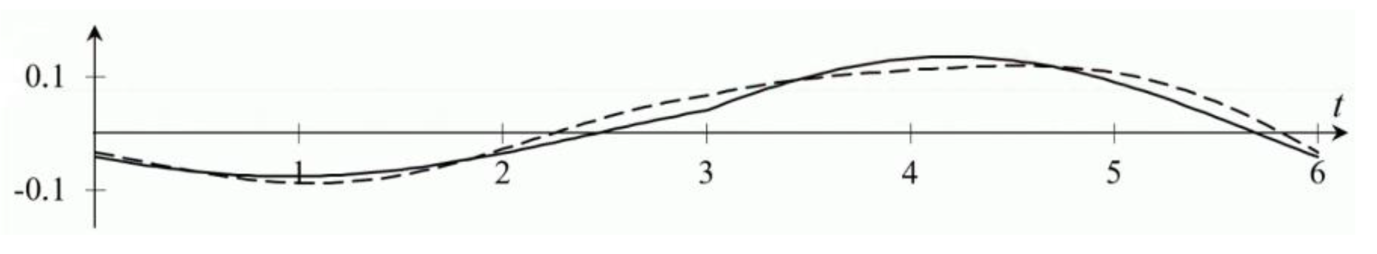
Let us illustrate the obtained formulas on the graphs. The graphs of the functions $u_1\left(t\right)$ and $u_2\left(t\right)$ are given in Figure 1.

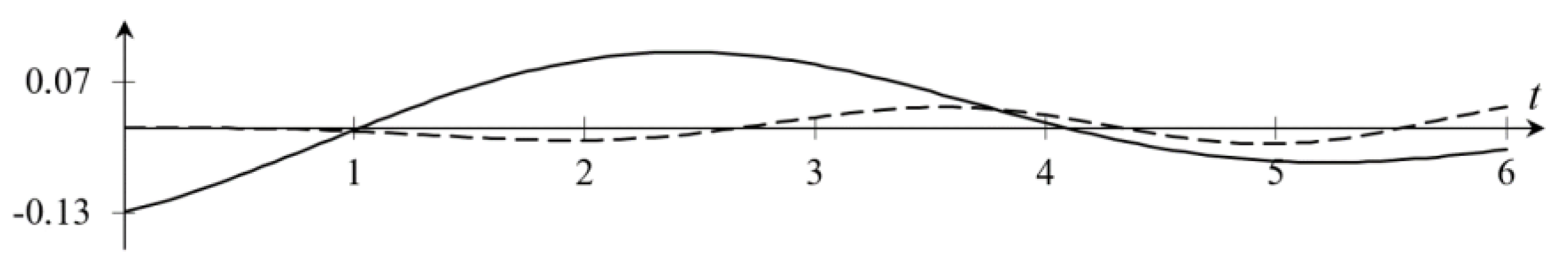
The graphs of the functions $V_1\left(t\right)$ and $V_2\left(t\right)$ are shown in Figure 2.

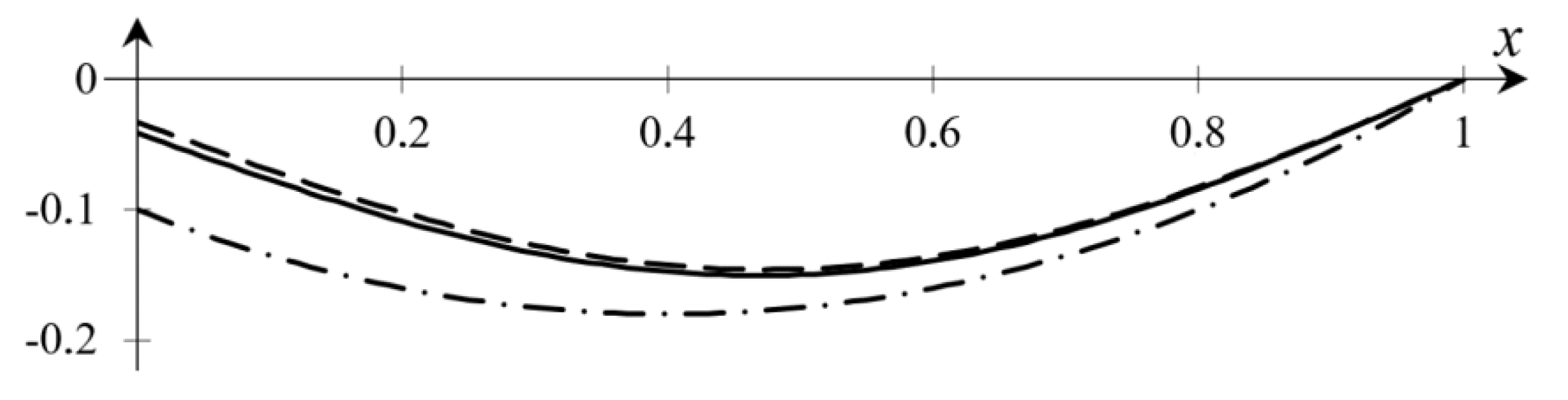
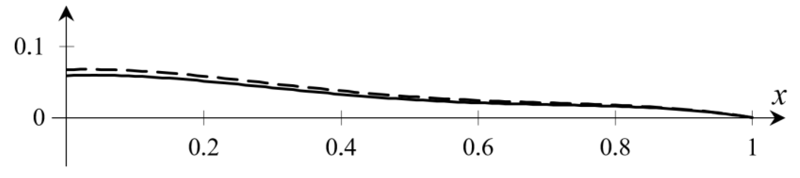
The graphical representation of the functions $Q_1\left(x,0\right)$, $Q_2\left(x,0\right)$ and $\hspace{0.17em}{\phi }_0\left(x\right)$ is illustrated in Figure 3.

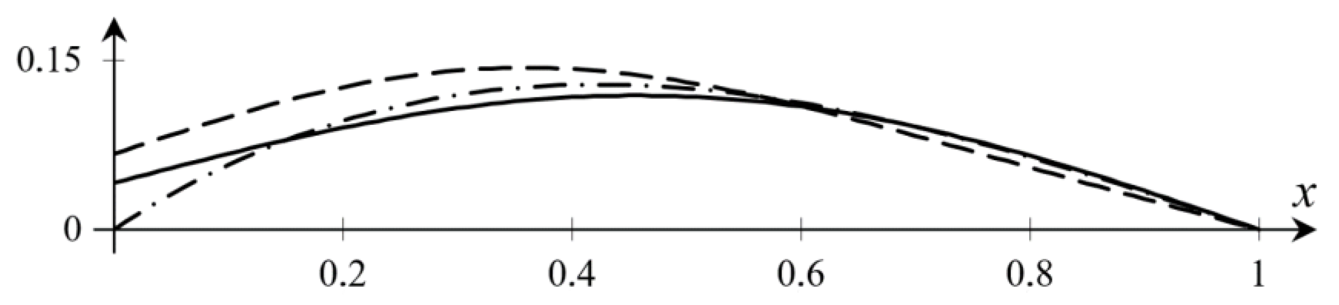
The graphs of the functions $Q_1\left(x,3\right)$, $Q_2\left(x,3\right)$ and ${\phi }_1\left(x\right)$ are shown in Figure 4, which illustrates the small discrepancies between these functions.

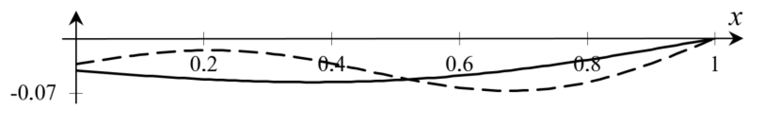
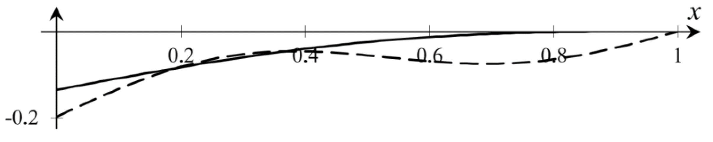
Graphical representations of the functions $Q_1\left(x,6\right)$ and $Q_2\left(x,6\right)$ and ${\dot{Q}}_1\left(x,6\right)$ and ${\dot{Q}}_2\left(x,6\right)$ are shown in Figure 5 and Figure 6, respectively.

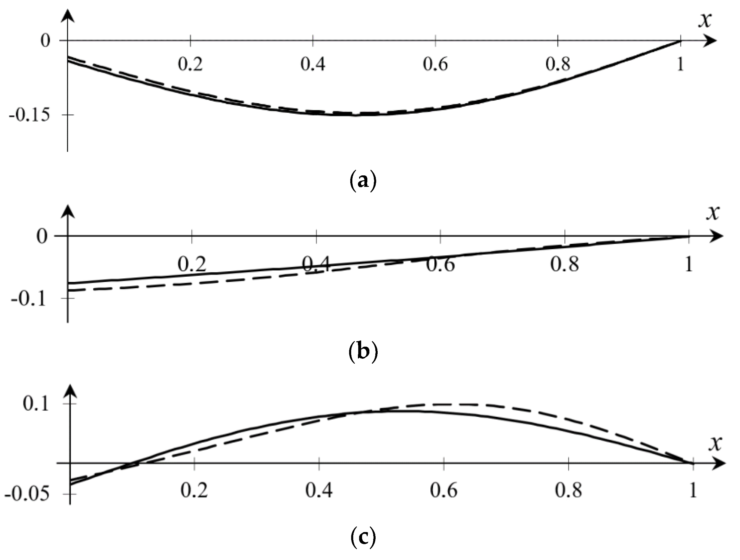
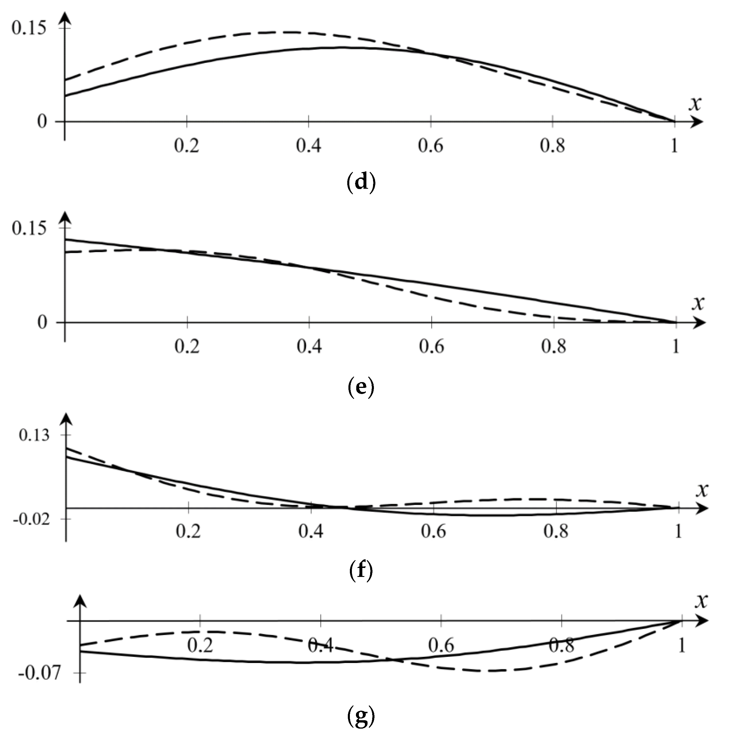
Figure 7 provides graphical illustrations of the dynamics of the behavior of the functions $Q_1\left(x,t\right)$ and $Q_2\left(x,t\right)$ given $t=0,\hspace{0.17em}1,\hspace{0.17em}2,\hspace{0.17em}3,\hspace{0.17em}4,\hspace{0.17em}5,\hspace{0.17em}6$.

5.4. Discussion of Results

For a comparative analysis of the results obtained, we denote by ${\epsilon }_n\left(x,\hspace{0.17em}{t}_j\right)=\left|Q_n\left(x,t_j\right)-{\phi }_j\left(x\right)\right|$ and ${\tilde{\epsilon }}_n\left(x,\hspace{0.17em}{t}_m\right)=\left|{\dot{Q}}_n\left(x,t_j\right)-{\psi }_m\left(x\right)\right|$, $n=1,2$, $m=0,2$, $j=\overline{0, 2}$ (here, $m=j=2$ corresponds to the moment of time $t_2=T$), which illustrate the discrepancy between these functions.

The maximum values of residuals ${\epsilon }_n\left(x,\hspace{0.17em}{t}_j\right)$, ${\tilde{\epsilon }}_n\left(x,\hspace{0.17em}{t}_m\right)$, $E_n\left(x,\hspace{0.17em}{t}_j\right)={{\displaystyle \int }}_0^1{\epsilon }_n\left(x,\hspace{0.17em}{t}_j\right)dx$ and ${\tilde{E}}_n\left(x,\hspace{0.17em}{t}_m\right)={{\displaystyle \int }}_0^1{\tilde{\epsilon }}_n\left(x,\hspace{0.17em}{t}_m\right)dx$ are given in the following table.

Table 1. Comparison of residuals for ${\phi }_j$.

	${\mathit{t}}_0=0$		${\mathit{t}}_1=3$		${\mathit{t}}_2=6$
	$\mathit{n}=1$	$\mathit{n}=2$	$\mathit{n}=1$	$\mathit{n}=2$	$\mathit{n}=1$	$\mathit{n}=2$
$\underset{0\le x\le 1}{\max }{\epsilon }_n\left(x,\hspace{0.17em}{t}_j\right)$	0.0589	0.0673	0.0411	0.0665	0.0559	0.0669
$\underset{0\le x\le 1}{\max }{E}_n\left(x,\hspace{0.17em}{t}_j\right)$	0.0307	0.0349	0.0068	0.0170	0.0413	0.0371

and

Table 2. Comparison of residuals for ${\psi }_m$.

	${\mathit{t}}_0=0$		${\mathit{t}}_2=6$
	$\mathit{n}=1$	$\mathit{n}=2$	$\mathit{n}=1$	$\mathit{n}=2$
$\underset{0\le x\le 1}{\max }{\tilde{\epsilon }}_n\left(x,\hspace{0.17em}{t}_m\right)$	0.0667	0.0714	0.1351	0.1970
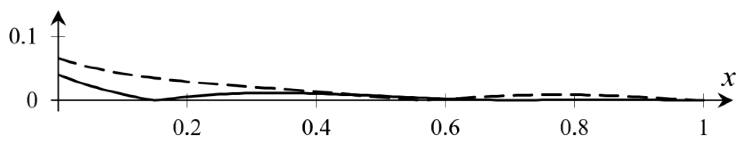
$\underset{0\le x\le 1}{\max }{\tilde{E}}_n\left(x,\hspace{0.17em}{t}_m\right)$	0.0341	0.0365	0.0402	0.0711

show that, under the constructed control, the behavior of the string deflection functions is quite close to that of the given initial ones. An illustration of the residuals at the initial and intermediate time points is shown in the following figures. The graphical representation of the functions ${\epsilon }_n\left(x,\hspace{0.17em}0\right)$, $n=1,2$, is shown in Figure 8.

The graphical representation of the functions ${\epsilon }_n\left(x,\hspace{0.17em}3\right)$, $n=1,2$, is shown in Figure 9.

The proposed analytical constructions are valid for any first $n$ harmonics of string vibrations. Numerical calculations, illustrations of the results and their analysis were carried out with the help of the developed general approach for $n=1,2$. The series (21) is uniformly convergent for functions from the above classes. The behavior of the functions $V_1\left(t\right)$ and $V_2\left(t\right)$ shows it (see Figure 2).

Thus, given $n=1$ and $n=2$, we construct explicit expressions of the boundary control $u_1\left(t\right)$ and $u_2\left(t\right)$ and those of the string deflection functions $Q_1\left(x,t\right)$ and $Q_2\left(x,t\right)$.

6. Conclusions

We proposed a constructive method for constructing the control of vibrations of a homogeneous string with a given deflection shape at an intermediate moment. We also proposed a constructive method for constructing the control of homogeneous string vibrations with a given deflection shape at an intermediate moment. The control was carried out by shifting one end with the other end fixed. The construction scheme was as follows: We reduced the original problem to the control problem of distributed influences with zero boundary conditions. Further, we used the method of separation of variables and methods of control theory for finite-dimensional systems with multipoint intermediate conditions.

We formulated the corresponding statement and theorem for the first $n$ harmonics. A specific example illustrated the obtained results. We realized a computational experiment, constructed the corresponding graphs and made a comparative analysis. They confirm the results of the study. The proposed method can be extended to other non-one-dimensional vibrational systems. The results presented in the paper can be used in the design of boundary control of vibration processes in physical and technological systems.

References

- Abdukarimov, M.F. On the optimal boundary control of displacements of the forced vibration process at the two ends of the string. Rep. Acad. Sci. Repub. Tajikistan 2013, 56, 612–618. [Google Scholar]
- Amara, J.B.; Beldi, E. Boundary controllability of two vibrating strings connected by a point mass with variable coefficients. SIAM J. Control Optim. 2019, 57, 3360–3387. [Google Scholar] [CrossRef] [Green Version]
- Andreev, A.A.; Leksina, S.V. The problem of boundary control for a system of wave equations. J. Samara State Tech. Univ. Ser. Phys. Math. Sci. 2008, 1, 5–10. [Google Scholar]
- Barseghyan, V.R.; Sahakyan, M.A. Optimal control of vibrations of a string with given states at intermediate moments of time. Proc. Natl. Acad. Sci. Repub. Armen. Mekhanika 2008, 61, 52–60. [Google Scholar]
- Barseghyan, V.R. Control Problem of String Vibrations with Inseparable Multipoint Conditions at Intermediate Points in Time. Mech. Solids 2019, 54, 1216–1226. [Google Scholar] [CrossRef]
- Barseghyan, V.R. The Problem of Optimal Control of String Vibrations. Int. Appl. Mech. 2020, 56, 471–480. [Google Scholar] [CrossRef]
- Barseghyan, V.R. The problem of control of rod heating process with nonseparated conditions at intermediate moments of time. Arch. Control. Sci. 2021, 31, 481–493. [Google Scholar] [CrossRef]
- Barseghyan, V.R. Control of Composite Dynamical Systems and Systems with Multipoint Intermediate Conditions; Nauka: Moscow, Russia, 2016. [Google Scholar]
- Barseghyan, V.R.; Barseghyan, T.V. On an approach to the problems of control of dynamic systems with nonseparated multipoint intermediate conditions. Automat. Remote. Control. 2015, 76, 549–559. [Google Scholar] [CrossRef]
- Butkovsky, A.G. Methods for Control of Systems with Distributed Parameters; Nauka: Moscow, Russia, 1975. [Google Scholar]
- Gibkina, N.V.; Sidorov, M.V.; Stadnikova, A.V. Optimal boundary control of homogeneous string vibrations. Radioelektron. Inform. 2016, 2, 3–11. [Google Scholar]
- Ilyin, V.A.; Moiseev, E.I. Optimization of boundary controls of string vibrations. Uspekhi Mat. Nauk. 2005, 60, 89–114. [Google Scholar] [CrossRef]
- Kopets, M.M. The problem of optimal control of the string vibration process. In Theory of Optimal Solutions: Collection of Research Contributions; Glushkov Institute of Cybernetics of the NAS of Ukraine: Kyiv, Ukraine, 2014; pp. 32–38. [Google Scholar]
- Moiseev, E.I.; Kholomeeva, A.A.; Frolov, A.A. Boundary displacement control for the oscillation process with boundary conditions of damping type for a time less than critical. J. Math. Sci. 2019, 160, 74–84. [Google Scholar] [CrossRef]
- Zhang, S.; He, W.; Li, G. Boundary control design for a flexible string system with input backlash. In Proceedings of the 2016 American Control Conference (ACC), Boston, MA, USA, 6–8 July 2016; pp. 6698–6702. [Google Scholar] [CrossRef]
- Zhao, Z. Boundary and distributed control for a vibrating string system. In Proceedings of the 2017 Chinese Automation Congress, Jinan, China, 20–22 October 2017; pp. 2099–2103. [Google Scholar] [CrossRef]
- Zhao, Z.; He, X.; Ahn, C.K. Boundary Disturbance Observer-Based Control of a Vibrating Single-Link Flexible Manipulator. In IEEE Transactions on Systems, Man, and Cybernetics: Systems; IEEE: Piscataway Township, NJ, USA, 2021; Volume 51, pp. 2382–2390. [Google Scholar] [CrossRef]
- Zhao, Z.; Shi, J.; Xiao, Y.; He, X.; He, W. Vibration control of flexible string systems with nonlinear input. In Proceedings of the 33rd Youth Academic Annual Conference of Chinese Association of Automation, Nanjing, China, 18–20 May 2018; pp. 230–234. [Google Scholar] [CrossRef]
- Znamenskaya, L.N. Control of Elastic Vibrations; FIZMATLIT: Moscow, Russia, 2004. [Google Scholar]
- Korzyuk, V.I.; Kozlovskaya, I.S. Two-point boundary problem for the equation of vibration of a string with a given velocity at a certain moment of time. I. Proc. Inst. Math. Natl. Acad. Sci. Belarus 2010, 18, 22–35. [Google Scholar]
- Korzyuk, V.I.; Kozlovskaya, I.S. Two-point boundary problem for the equation of string vibration with a given velocity at a certain moment of time. II. Proc. Inst. Math. Natl. Acad. Sci. Belarus 2011, 19, 62–70. [Google Scholar]
- Muravey, L.A.; Petrov, V.M.; Romanenkov, A.M. The Problem of Damping the Transverse Oscillations on a Longitudinally Moving String. Mordovia Univ. Bull. 2018, 28, 472–485. [Google Scholar] [CrossRef]
- Tikhonov, A.N.; Samarskii, A.A. Equations of Mathematical Physics; Dover Publications: Mineola, NY, USA, 2011. [Google Scholar]
- Zubov, V.I. Lectures on Control Theory; Nauka: Moscow, Russia, 1975. [Google Scholar]