Stability and Hopf Bifurcation Analysis of a Stage-Structured Predator–Prey Model with Delay

Abstract

In this work, a Lotka–Volterra type predator–prey system with time delay and stage structure for the predators is proposed and analyzed. By using the permanence theory for infinite dimensional system, we get that the system is permanent if some conditions are satisfied. The local and global stability of the positive equilibrium is presented. The existence of Hopf bifurcation around the positive equilibrium is observed. Further, by using the normal form theory and center manifold approach, we derive the explicit formulas determining the stability of bifurcating periodic solutions and the direction of Hopf bifurcation. Numerical simulations are carried out by Matlab software to explain the theoretical results. We find that combined time delay and stage structure can affect the dynamical behavior of the system.

1. Introduction

Differential equations are a powerful tool for characterizing natural phenomena [1,2]. The predator–prey model is a very classic model, which plays a key role in population ecology. Many predator–prey models have been investigated by some researchers [3,4,5,6,7,8,9]. From [10], we know that if the following classical autonomous Lotka–Volterra type predator prey model,

$$\begin{array}{c}\hfill \left\{\begin{array}{c}\frac{dx(t)}{dt}=x(t)[k-x(t)-\alpha y(t)],\hfill \\ \frac{dy(t)}{dt}=y(t)[-r+\beta x(t)-y(t)],\hfill \end{array}\right.\end{array}$$

(1)

exists in a positive equilibrium $(x^1,y^1)$, it must be globally asymptotically stable. Time lag is pervasive in nature. The stability issues for the Lotka-Volterra system with different types of time delays have been extensively studied. In [11], by using Lyapunov functional, He examined the global attraction for a kind of delayed n-species Lotka–Volterra-type system. In [12], Gopalsamy et al. examined the global stability of a delay nonautonomous n-species competition system. In [13], He investigated the global asymptotic stability of a nonautonomous Lotka–Volterra system with “pure-delay type”. In [14], Wang et al. proved that delays are harmless for the two-dimensional delayed Lotka–Volterra system. As a special case of Lotka–Volterra-type systems with delays, Chen et al. proposed a model of two species’ growth delays as a reasonable generalization of the Lotka–Volterra model, which takes the form [10]:

$$\begin{array}{c}\hfill \left\{\begin{array}{c}\frac{dx(t)}{dt}=x(t)[k-x(t)-\alpha y(t-\tau )],\hfill \\ \frac{dy(t)}{dt}=y(t)[-r+\beta x(t-\tau )-y(t)].\hfill \end{array}\right.\end{array}$$

(2)

System (2) is one of the simplest predator–prey models with a delay. Its stability and Hopf bifurcations, both local and global, have been widely investigated. For example, Wang et al. [14] found that system (2) was uniformly persistent irrespective of the size of the delays. He [11] showed that the positive equilibrium is locally and globally asymptotically stable.

In the real world, however, many consumer species may go though multiple life phases as they progress from birth to death. In [15,16], the authors studied the delayed stage structure models. In those models, a constant time lag represented the time from birth to maturity. References [17,18] have examined the stage structure of species when the transformation rate of the mature population is proportional to the existing immature population. Motivated by the works of Chen [10], He et al. [11,12,13], Cui et al. [15] and Song et al. [16], we built a predator–prey model based on system (2), which includes a time delay due to negative feedback of prey and the stage structure for the predators. This paper’s purpose is to explore the combined effects of both delay and stage structure on the predator–prey system’s dynamical behavior.

2. The Model

We consider a delayed predator–prey system with a stage structure among predator populations of the following form:

$$\begin{array}{c}\hfill \left\{\begin{array}{c}\frac{dx(t)}{dt}=x(t)[k-x(t)-\alpha y(t-\tau )],\hfill \\ \frac{dy(t)}{dt}=y(t)[-r+\beta x(t-\tau )-y(t)]+\sigma y_i(t),\hfill \\ \frac{d{y}_i(t)}{dt}=cy(t)-(\sigma +\gamma )y_i(t),\hfill \end{array}\right.\end{array}$$

(3)

where $x(t)$ expresses prey density at time t, and $y(t)$ and $y_i(t)$ represent densities of the mature and the immature predator species at time t. In model (3), $\alpha$ and $\beta$ represent the capturing rates of the predators; k is the intrinsic rate of increase for the prey; r represents the mature predator’s death rate; $\sigma$ represents the conversion rate; $\gamma$ is the immature predator’s death rate; c denotes the birth rate of the immature predators; $\tau$ is a constant delay. All the parameters (i.e., k, $\alpha$, r, $\sigma$, $\beta$, c, $\gamma$, and $\tau$) are positive constants.

The initial conditions for system (3) have the following form:

$$\begin{array}{c}\hfill \begin{array}{c}x(\varsigma )={\phi }_1(\varsigma )\ge 0,y(\varsigma )={\phi }_2(\varsigma )\ge 0,y_i(\varsigma )={\phi }_2(\varsigma )\ge 0,\varsigma \in [-\tau ,0],\hfill \\ {\phi }_1(0)>0,{\phi }_2(0)>0.\hfill \end{array}\end{array}$$

(4)

We suppose that $z(t)=(x(t),y(t),y_i(t))$ is the solution of system (3) with the initial conditions (4). Obviously, under the initial conditions given in (4), the solution $z(t)$ of system (3) exists in the interval $[0,+\infty )$. Further, it remains positive for all $t\ge 0$. In fact, from the 1st equation of (3), we obtain

$$x(t)=x(0)exp({\int }_0^t(k-x(s)-\alpha y(s-\tau ))ds)>0$$

for $t\ge 0$. Set $\Xi (t)=-r+\beta x(t-\tau )-y(t)$, we can rewrite the last two equations of (3) as

$$\begin{array}{c}\hfill \left\{\begin{array}{c}\frac{dy(t)}{dt}=\Xi (t)y(t)+\sigma y_i(t),\hfill \\ \frac{d{y}_i(t)}{dt}=cy(t)-(\sigma +\gamma )y_i(t).\hfill \end{array}\right.\end{array}$$

(5)

Obviously, there is a unique solution $z(t)$ of system (3) in a maximal interval $[0,d)$ [19]. We can prove that the interval is $[0,+\infty )$. Since (5) is a quasimonotone system, $(0,0)$ is a subsolution and $w(e^{at},e^{at})$ with $w>y(0),y_i(0)$ and $a>\sigma ,$ $\sigma$ is a supersolution [19]. This shows that $y(t)$ and $y_i(t)$ are bounded in $[0,d)$ and hence exist for all $t>0$. Suppose $y_i(b)=0$. We can obtain $\frac{d{y}_i(t)}{dt}{|}_{t=b}=0$ and $y(b)=0$. This shows that $(y(t),y_i(t))$ is a solution of (5) at $t=b$ and hence it is zero in $(0,+\infty )$. This is a contradiction. Hence, $y(t)>0$, $y_i(t)>0$ for $t>0$. Thereby, $x(t)>0$ for $t>0$.

It is straightforward to see that in system (3) there exist four equilibrium points

$$\begin{array}{cccc}{E}_0(0,0,0),\hfill & E_1(k,0,0),\hfill & E_2(0,y^0,y_i^0),\hfill & E^{*}(x^{*},y^{*},y_i^{*}),\hfill \end{array}$$

where

$$\begin{array}{cc}{y}^0=\frac{-r(\sigma +\gamma )+\sigma c}{\sigma +\gamma },y_i^0=\frac{c(-r(\sigma +\gamma )+\sigma c)}{{(\sigma +\gamma )}^2},\hfill & \\ x^{*}=\frac{(k+\alpha r)(\sigma +\gamma )-\sigma c\alpha }{(1+\alpha \beta )(\sigma +\gamma )},y^{*}=\frac{(-r+k\beta )(\sigma +\gamma )+\sigma c}{(1+\alpha \beta )(\sigma +\gamma )},y_i^{*}=\frac{c((-r+\beta k)(\sigma +\gamma )+\sigma c)}{(1+\alpha \beta ){(\sigma +\gamma )}^2}.\hfill \end{array}$$

If the conditions

$$\begin{array}{c}\hfill (k+\alpha r)(\sigma +\gamma )-c\sigma \alpha >0\end{array}$$

(6)

and

$$\begin{array}{c}\hfill -r(\sigma +\gamma )+c\sigma >0\end{array}$$

(7)

hold, all the equilibria are nonnegative.

3. Permanence of System (3)

We first introduce the definition of permanence.

Definition 1

([20]). System (3) is permanent if there exist positive constants ${\mathcal{M}}_1$ and ${\mathcal{M}}_2$ such that any positive solution $(x(t),y(t),y_i(t))$ of system (3) with initial conditions (4) satisfies

$${\mathcal{M}}_1\le \underset{t\to +\infty }{lim\; inf}x(t)\le \underset{t\to +\infty }{lim\; sup}x(t)\le {\mathcal{M}}_2,$$

$${\mathcal{M}}_1\le \underset{t\to +\infty }{lim\; inf}y(t)\le \underset{t\to +\infty }{lim\; sup}y(t)\le {\mathcal{M}}_2,$$

$${\mathcal{M}}_1\le \underset{t\to +\infty }{lim\; inf}{y}_i(t)\le \underset{t\to +\infty }{lim\; sup}{y}_i(t)\le {\mathcal{M}}_2.$$

Theorem 1.

Any positive solution $(x(t),y(t),y_i(t))$ of system (3) with initial condition (4) satisfies $0<x(t),y(t),y_i(t)\le M$ for $t\ge 0$.

Proof. 

Suppose $(x(t),y(t),y_i(t))$ is a positive solution of system (3) with initial condition (4). According to the first equation of system (3), it follows from the positivity of the solution that

$$\dot{x}(t)\le x(t)(k-x(t)).$$

The solution of the auxiliary equation

$$\dot{u}(t)=u(t)(k-u(t)),u(0)=x(0)>0$$

has the following properties: there exist $\epsilon >0$ and $T>0$ such that $u(t)<k+\epsilon$ for $t\le T$. Hence, by comparing the theorems for ordinary differential equations, we have $x(t)\le u(t)<k+\epsilon$ for $t\le T$.

Denote $M_1=k+\epsilon$. Then,

$$\begin{array}{c}\hfill x(t)\le M_1.\end{array}$$

(8)

It follows from (8) and the second equation of system (3) that for $t\le T$,

$$\begin{array}{c}\hfill \dot{y}(t)\le y(-r+\beta M_1-y)+\sigma y_i.\end{array}$$

(9)

We define

$$V_1(t)=(\sigma +\gamma )y+\sigma y_i.$$

Along the last two equations of system (3), we calculate the upper-right derivative of $V_1$:

$$\begin{array}{cc}{D}^{+}{V}_1(t)\hfill & =(\sigma +\gamma )\dot{y}+\sigma \dot{y_i}\hfill \\ & \le (\sigma +\gamma )y(-r+\beta M_1-y)+\sigma cy\hfill \\ & \le \frac{{[(\sigma +\gamma )(-r+\beta M_1)+\sigma c]}^2}{4(\sigma +\gamma )}.\hfill \end{array}$$

Then, there exist two positive constants $M_2$, $M_3$, such that

$$0<y(t)\le M_2,0<y_i(t)\le M_3.$$

Denote $M=min\{M_1,M_2,M_3\}$. Then, $0<x(t),y(t),y_i(t)\le M$ for $t\ge 0$.

Next, we discuss the permanence of system (3).

To prove that system (3) is persistent, we will use Theorem 4.1 in [20]. □

Theorem 2.

If condition (6) and

$$\begin{array}{c}\hfill -r+k\beta >0\end{array}$$

(10)

hold, then system (3) is permanent.

Proof. 

We begin by showing that sets $X_1$, $X_2$, $X_3$ and $X_4$ repel the positive solution of system (3) uniformly. Let us define

$$\begin{array}{cc}& C_1=\{({\phi }_1,{\phi }_2,{\phi }_3)\in C([-\tau ,0],{\mathbb{R}}_{+}^3):{\phi }_2(\theta )=0\},\hfill \\ & C_2=\{({\phi }_1,{\phi }_2,{\phi }_3)\in C([-\tau ,0],{\mathbb{R}}_{+}^3):{\phi }_1(\theta )=0\},\hfill \\ & X_1=\{(x,y,y_i)\in {\mathbb{R}}^3\mid x>0,y=0,y_i>0\},\hfill \\ & X_2=\{(x,y,y_i)\in {\mathbb{R}}^3\mid x=0,y>0,y_i>0\},\hfill \\ & X_3=\{(x,y,y_i)\in {\mathbb{R}}^3\mid x=0,y>0,y_i=0\},\hfill \\ & X_4=\{(x,y,y_i)\in {\mathbb{R}}^3\mid x=0,y=0,y_i>0\},\hfill \\ & C_0=C_1\cup C_2,C^0=\mathrm{Int}C([-\tau ,0],{\mathbb{R}}_{+}^3),\hfill \\ & X_0=X_1\bigcup X_2\bigcup X_3\bigcup X_4,X^0=\{(x,y,y_i)\in {\mathbb{R}}^3\mid x>0,y>0,y_i>0\}.\hfill \end{array}$$

This choice meets the conditions in Theorem 4.1 in [20]. It suffices to show that, for any solution $z(t)=(x(t),y(t),y_i(t))$ of system (3) initiating from $C^0$, there exists an ${\epsilon }_0>0$ such that $\underset{t\to +\infty }{lim\; inf}d(z(t),X_0)\ge {\epsilon }_0$. To this end, we shall verify that all the conditions of Theorem 4.1 in [20] are satisfied. It is easy to see that $C^0$ and $C_0$ are positively invariant. Obviously, conditions $(i)$ and $(ii)$ of Theorem 4.1 in [20] are satisfied. In the following, we shall only need to validate conditions $(iii)$ and $(iv)$.

There are three constant solutions, $E_0(0,0,0)$, $E_1(k,0,0)$, $E_2(0,y^0,y_i^0)$, in $X_0$.

In the set $X_3$ or $X_4$, system (3) becomes

$$\dot{y}=y(-r-y)\mathrm{or}{\dot{y}}_i=-(\sigma +\gamma )y_i.$$

Clearly, $\underset{t\to +\infty }{lim}y(t)=0$, $\underset{t\to +\infty }{lim}{y}_i(t)\to 0$. Hence, for any solution $(x(t),y(t),y_i(t))$ of system (3) initiating from $C_0$, we obtain $(x(t),y(t),y_i(t))\to E_0(0,0,0)$ as $t\to +\infty$.

In the set $X_1$, system (3) becomes

$$\left\{\begin{array}{c}\dot{x}(t)=x(t)(k-x(t)),\hfill \\ \dot{y_i}(t)=-(\sigma +\gamma )y_i(t).\hfill \end{array}\right.$$

Obviously, $E_1(k,0)$ is globally asymptotically stable. Therefore, any solution $(x(t),y(t),y_i(t))$ of system (3) initiating from $C_1$ is such that $(x(t),y(t),y_i(t))\to E_1(k,0,0)$ as $t\to +\infty$.

In the set $X_2$, system (3) becomes

$$\left\{\begin{array}{c}\dot{y}(t)=y(t)(-r-y(t))+\sigma y_i(t),\hfill \\ \dot{y_i}(t)=cy(t)-(\sigma +\gamma )y_i(t).\hfill \end{array}\right.$$

Clearly, $E_2(y^0,y_i^0)$ is globally asymptotically stable. Hence, for any solution $(x(t),y(t),y_i(t))$ of system (3) which initiates from $C_2$, we have $(x(t),y(t),y_i(t))\to E_2(0,y^0,y_i^0)$ as $t\to +\infty$.

Obviously, $E_0,E_1,E_2$ are isolated invariant, and $\{E_0,E_1,E_2\}$ is isolated and is an acyclic covering.

It is obvious that $W^s(E_0)\bigcap X^0=\varnothing$. Next, we will show that $W^s(E_1)\bigcap X^0=\varnothing$, $W^s(E_2)\bigcap X^0=\varnothing$.

Assume $W^s(E_q)\bigcap X^0\ne \varnothing$. Then, in system (3) there exists a positive solution $(\overline{x}(t),\overline{y}(t),{\overline{y}}_i(t))$ such that $(\overline{x}(t),\overline{y}(t),{\overline{y}}_i(t))$ $\to E_1(k,0,0)$ as $t\to +\infty$. Hence, we have $\underset{t\to +\infty }{lim}x(t)=k$, that is, for $\epsilon >0$, there exists $t_0>0$ such that $\overline{x}(t)>k-\epsilon$. From system (3), for $t>t_0+\tau$,

$$\dot{y}(t)\ge y(t)(-r+\beta (k-\epsilon )-y(t)).$$

From (10), we can find that $\overline{y}(t)\to -r+k\beta .$ This is a contradiction. Therefore, we have $W^s(E_1)\bigcap X^0=\varnothing$.

Assume $W^s(E_2)\cap X^0\ne \varnothing$. Then, there is a positive solution $(\overline{x}(t),\overline{y}(t),{\overline{y}}_i(t))$ of (3) that $(\overline{x}(t),\overline{y}(t),{\overline{y}}_i(t))\to E_2(0,y^0,y_i^0)$ as $t\to +\infty$. Hence, $y\to y^0$, $y\to y_i^0$ as $t\to +\infty$. From system (3), for $t>t_0+\tau$, we have

$$\dot{x}(t)\ge x(t)(k-x(t)-\alpha (y^0+\epsilon )).$$

From (6), we find that $\overline{x}(t)\to k-\alpha y^0$ as $t\to +\infty$. This is a contradiction. Therefore, we have $W^s(E_2)\bigcap X^0=\varnothing$.

At this time, we can conclude that $X_0$ repels the positive solutions $(x(t),y(t),y_i(t))$ of system (3) which initiates from $C^0$ uniformly.

Thus, there exists an ${\epsilon }_0>0$ such that

$$\underset{t\to +\infty }{lim\; inf}x(t)\ge {\epsilon }_0,\underset{t\to +\infty }{lim\; inf}y(t)\ge {\epsilon }_0.$$

From the 3rd equation of system (3), we obtain

$${\dot{y}}_i(t)\ge c{\epsilon }_0-(\gamma +\sigma )y_i(t).$$

Then $y_i\to \frac{c{\epsilon }_0}{\gamma +\sigma }$ as $t\to +\infty$. Denote ${\epsilon }_1=\frac{c{\epsilon }_0}{\gamma +\sigma }$, then $y_i\ge {\epsilon }_1$. □

4. Stability of Equilibria

In this section, we will discuss the sufficient conditions for the stability of all the equilibrium points for system (3).

Firstly, we analyze the local stability of the equilibria $E_0$, $E_1$, $E_2$.

The characteristic equation of equilibrium $E_0$ is

$$(\lambda -k)({\lambda }^2+(\sigma +\gamma +r)\lambda +r(\sigma +\gamma )-\sigma c)=0.$$

Obviously, the above equation always has a positive eigenvalue $\lambda =k$. Hence, $E_0(0,0,0)$ is unstable.

The characteristic equation of equilibrium $E_1$ is

$$\begin{array}{c}\hfill (\lambda +k)[{\lambda }^2+(r-\beta k+\sigma +\gamma )\lambda +(r-\beta k)(\sigma +\gamma )-\sigma c]=0.\end{array}$$

(11)

Let

$$f(\lambda )={\lambda }^2+(r-\beta k+\sigma +\gamma )\lambda +(r-\beta k)(\sigma +\gamma )-\sigma c.$$

From (7), we can find $(r-\beta k)(\sigma +\gamma )-\sigma c<0$. Then, $f(+\infty )=+\infty$, $f(0)<0$. So (11) has a positive root, i.e., the equilibrium $E_1(k,0,0)$ is unstable.

The characteristic equation of equilibrium $E_2$ is

$$\begin{array}{c}\hfill (\lambda -k+\alpha y^0)[{\lambda }^2+(r+2y^0+\sigma +\gamma )\lambda +(r+2y^0)(\sigma +\gamma )-\sigma c]=0.\end{array}$$

(12)

Denote

$$f(\lambda )={\lambda }^2+(r+2y^0+\sigma +\gamma )\lambda +(r+2y^0)(\sigma +\gamma )-\sigma c.$$

Then, $f(+\infty )=+\infty$, $f(0)<0$, so (13) has a positive root. Then the equilibrium $E_2$ is unstable.

In the following, we shall discuss the local and global properties of positive equilibrium $E^{*}$.

Theorem 3.

The interior equilibrium $E^{*}(x^{*},y^{*},y_i^{*})$ of system (3) is locally asymptotically stable if conditions (6) and (7) and the condition

$$\begin{array}{c}\hfill \alpha \beta <1\end{array}$$

(13)

hold.

Proof. 

Linearizing system (3) at the equilibrium $E^{*}(x^{*},y^{*},y_i^{*})$ leads to

$$\begin{array}{c}\hfill \left\{\begin{array}{c}\dot{x}(t)=-x^{*}x(t)-\alpha x^{*}y(t-\tau ),\hfill \\ \dot{y}(t)=\beta y^{*}x(t-\tau )+(-r+\beta x^{*}-2y^{*})y(t)+\sigma y_i(t),\hfill \\ \dot{y_i}(t)=cy(t)-(\sigma +\gamma )y_i(t).\hfill \end{array}\right.\end{array}$$

(14)

We obtain the characteristic equation of the form

$$\begin{array}{c}\hfill \Gamma (\lambda ,\tau )={\lambda }^3+p{\lambda }^2+q\lambda +s+e^{-2\lambda \tau }(l\lambda +n)=0,\end{array}$$

(15)

where

$$\begin{array}{cc}& p=\sigma +\gamma +\frac{c\sigma }{\sigma +\gamma }+x^{*}+y^{*}>0,\hfill \\ & q=(x^{*}+y^{*})(\sigma +\gamma )+x^{*}(\frac{c\sigma }{\sigma +\gamma }+y^{*})>0,\hfill \\ & s=x^{*}{y}^{*}(\sigma +\gamma )>0,\hfill \\ & l=x^{*}{y}^{*}\alpha \beta >0,\hfill \\ & n=x^{*}{y}^{*}\alpha \beta (\sigma +\gamma )>0.\hfill \end{array}$$

When $\tau =0$, we can easily check that all the characteristic roots have negative real parts. We will show that all the characteristic roots have negative real parts for all $\tau >0$, which implies that $E^{*}(x^{*},y^{*},y_i^{*})$ is locally asymptotically stable for (3). Obviously, the characteristic Equation (15) has no positive real parts roots. Now, we suppose that there exists a characteristic root of (15) on the imaginary axis of the complex plane for some ${\tau }_0>0$. Let $\lambda =i\omega$ be such a characteristic root. It is straightforward to see that $\omega \ne 0$. Substituting $(\lambda ,\tau )=(i\omega ,{\tau }_0)$ into (15) and separating the real and imaginary parts, we obtain

$$-p{\omega }^2+s+ncos(2\omega {\tau }_0)+l\omega sin(2\omega {\tau }_0)=0,$$

and

$$-{\omega }^3+q\omega +\omega lcos(2\omega {\tau }_0)-nsin(2\omega {\tau }_0)=0.$$

Furthermore,

$$\begin{array}{c}\hfill \begin{array}{cc}& (l^2{\omega }^2+n^2)sin(2\omega {\tau }_0)=pl{\omega }^3-ls\omega -n{\omega }^3+q\omega n,\hfill \\ & (l^2{\omega }^2+n^2)cos(2\omega {\tau }_0)=l{\omega }^4-ql{\omega }^2+p{\omega }^{2}n-ns.\hfill \end{array}\end{array}$$

(16)

Squaring and adding the two equations yields

$$\begin{array}{c}\hfill {(l^2{\omega }^2+n^2)}^2={(pl{\omega }^3-ls\omega -n{\omega }^3+q\omega n)}^2+{(l{\omega }^4-ql{\omega }^2+p{\omega }^{2}n-ns)}^2.\end{array}$$

(17)

Let $\Omega ={\omega }^2$ and

$$\begin{array}{c}\hfill \begin{array}{cc}f(\Omega )=\hfill & {\Omega }^3+(p^2-2q){\Omega }^2+(q^2-2ps-l^2)\Omega +s^2-n^2=0.\hfill \end{array}\end{array}$$

(18)

Then, $f(\Omega )$ must have a positive zero $\Omega ={\omega }^2$ because (17) and $\omega \ne 0$. What is more, the coefficients of ${\Omega }^2$, $\Omega$ and $f(0)$ in (18) need to be positive. In fact, the coefficients of ${\Omega }^2$ and $\Omega$ are expressed in the following ways:

$$\begin{array}{cc}& p^2-2q={(\sigma +\gamma )}^2+{(\frac{c\sigma }{\sigma +\gamma })}^2+x^{*}{}^2+y^{*}{}^2+2c\sigma +\frac{2c\sigma }{\sigma +\gamma }{y}^{*}>0,\hfill \\ & q^2-2ps-l^2=x^{*}{}^2{(\sigma +\gamma )}^2+y^{*}{}^2{(\sigma +\gamma )}^2+{(\frac{c\sigma x^{*}}{\sigma +\gamma })}^2+2x^{*}{}^{2}c\sigma +\frac{2c\sigma x^{*}{}^2{y}^{*}}{\sigma +\gamma }\hfill \\ & +(1-{\alpha }^2{\beta }^2)x^{*}{}^2{y}^{*}{}^2>0.\hfill \end{array}$$

Furthermore,

$$f(0)=s^2-n^2={(\sigma +\gamma )}^2{x}^{*}{}^2{y}^{*}{}^2(1-{\alpha }^2{\beta }^2)>0.$$

Hence, $f^{\prime }(\Omega )>0$. Therefore, $f(\Omega )=0$ has no positive roots, which is a contradiction. We complete the proof. □

Theorem 4.

Suppose that (6) and (7) and

$$\begin{array}{c}\hfill \alpha +\beta <2\end{array}$$

(19)

hold. Then the positive equilibrium $E^{*}(x^{*},y^{*},y_i^{*})$ of system (3) is globally asymptotically stable.

Proof. 

Let $(x(t),y(t),y_i(t))$ be any solution of system (3) satisfying initial condition (4). Define

$$\begin{array}{c}\hfill \begin{array}{cc}V(t)\hfill & ={\lambda }_1(x-x^{*}-x^{*}ln\frac{x}{x^{*}})+{\lambda }_2(y-y^{*}-y^{*}ln\frac{y}{y^{*}})+{\lambda }_3(y_i-y_i^{*}-y_i^{*}ln\frac{y_i}{y_i^{*}})\hfill \\ & {\displaystyle +\frac{{\lambda }_2\beta }{2}{\int }_{t-\tau }^t{(x^{*}-x(s))}^{2}ds+\frac{{\lambda }_1\alpha }{2}{\int }_{t-\tau }^t{(y^{*}-y(s))}^{2}ds,}\hfill \end{array}\end{array}$$

(20)

where ${\lambda }_1$, ${\lambda }_2$, ${\lambda }_3$ are suitable positive constants to be determined in the subsequent steps. It is easy to see that V is a positive definite function in the region $R_{+}^3$ except at $E^{*}(x^{*},y^{*},y_i^{*})$ where it vanishes. Further,

$$\underset{x\to 0,y\to 0,y_i\to 0}{lim}V(x,y,y_i)=\underset{x\to \infty ,y\to \infty ,y_i\to \infty }{lim}V(x,y,y_i)=\infty .$$

Calculating the upper right derivative of V along the solutions of system (3), we have:

$$\begin{array}{cc}{D}^{+}{V(t)|}_{(3)}\hfill & ={\lambda }_1(x-x^{*})(k-x-\alpha y(t-\tau ))+{\lambda }_2(y-y^{*})[(-r+\beta x(t-\tau )-y)+\frac{\sigma y_i}{y}]\hfill \\ & +{\lambda }_3(y_i-y_i^{*})(\frac{cy}{y_i}-(\sigma +\gamma ))+\frac{{\lambda }_2\beta }{2}[{(x-x^{*})}^2-{(x(t-\tau )-x^{*})}^2]\hfill \\ & +\frac{{\lambda }_1\alpha }{2}[{(y^{*}-y)}^2-{(y(t-\tau )-y^{*})}^2]\hfill \\ & =-{\lambda }_1{(x-x^{*})}^2+{\lambda }_1(x-x^{*})(\alpha y^{*}-\alpha y(t-\tau ))-{\lambda }_2{(y-y^{*})}^2+\hfill \\ & {\lambda }_2(y-y^{*})(\beta x(t-\tau )-\beta x^{*}-\frac{c\sigma }{\sigma +\gamma }+\frac{\sigma y_i}{y})+{\lambda }_3(y_i-y_i^{*})(\frac{cy}{y_i}-(\sigma +\gamma ))\hfill \\ & +\frac{{\lambda }_2\beta }{2}[{(x-x^{*})}^2-{(x(t-\tau )-x^{*})}^2]+\frac{{\lambda }_1\alpha }{2}[{(y^{*}-y)}^2-{(y(t-\tau )-y^{*})}^2]\hfill \\ & \le -{\lambda }_1{(x-x^{*})}^2+\frac{{\lambda }_1\alpha }{2}{(x-x^{*})}^2-{\lambda }_2{(y-y^{*})}^2+\frac{{\lambda }_2\beta }{2}{(y-y^{*})}^2+\frac{{\lambda }_2\beta }{2}{(x-x^{*})}^2\hfill \\ & +\frac{{\lambda }_1\alpha }{2}{(y-y^{*})}^2+\frac{{\lambda }_2(y-y^{*})}{(\sigma +\gamma )y}[(\sigma +\gamma )\sigma y_i-c\sigma y]+\frac{{\lambda }_3(y_i-y_i^{*})}{y_i}(cy-(\sigma +\gamma )y)\hfill \\ & =(-{\lambda }_1+\frac{{\lambda }_1\alpha }{2}+\frac{{\lambda }_1\beta }{2}){(x-x^{*})}^2+(-{\lambda }_2+\frac{{\lambda }_2\alpha }{2}+\frac{{\lambda }_2\beta }{2}){(y-y^{*})}^2\hfill \\ & -[\frac{{\lambda }_2\sigma y^{*}{y}_i-{\lambda }_3(\sigma +\gamma )y{y}_i^{*}}{(\sigma +\gamma )y{y}_i}+\frac{{\lambda }_3(\sigma +\gamma )y{y}_i-{\lambda }_2\sigma y{y}_i}{(\sigma +\gamma )y{y}_i}](cy-(\sigma +\gamma )y_i).\hfill \end{array}$$

Let ${\lambda }_2\sigma ={\lambda }_3(\sigma +\gamma )$. Then,

$$\begin{array}{cc}{D}^{+}{V(t)|}_{(3)}\hfill & \le (-{\lambda }_1+\frac{{\lambda }_1\alpha }{2}+\frac{{\lambda }_2\beta }{2}){(x-x^{*})}^2+(-{\lambda }_2+\frac{{\lambda }_1\alpha }{2}+\frac{{\lambda }_2\beta }{2}){(y-y^{*})}^2\hfill \\ & -\frac{{\lambda }_2\sigma y^{*}{y}_i-{\lambda }_3(\sigma +\gamma )y{y}_i^{*}}{(\sigma +\gamma )y{y}_i}(cy-(\sigma +\gamma )y_i)\hfill \\ & =(-{\lambda }_1+\frac{{\lambda }_1\alpha }{2}+\frac{{\lambda }_2\beta }{2}){(x-x^{*})}^2+(-{\lambda }_2+\frac{{\lambda }_1\alpha }{2}+\frac{{\lambda }_2\beta }{2}){(y-y^{*})}^2\hfill \\ & -\frac{{\lambda }_2\sigma y^{*}{y}_i}{{(\sigma +\gamma )}^{2}y{y}_i}{(cy-(\sigma +\gamma )y_i)}^2.\hfill \end{array}$$

Let ${\lambda }_1={\lambda }_2$. If (19) holds, then

$$D^{+}{V(t)|}_{(3)}<0.$$

Therefore, by using a Lyapunov–Lasalle type theorem [21], we have $x\to x^{*}$, $y\to y^{*}$, $y_i\to y_i^{*}$ as $t\to \infty$. □

5. Existence of Hopf Bifurcation

In this section, we shall find the conditions under which a Hopf bifurcation may occur around the positive equilibrium point $E^{*}$ when delay $\tau$ passes through some critical values.

From (18) we can see that if $1-\alpha \beta <0$ and $q^2-2ps-l^2>0$, then $f(0)=s^2-n^2<0$, $f(+\infty )=+\infty$ and $f^{\prime }(0)>0$. Hence, Equation (15) has a unique positive root. Then, we have the following lemma.

Lemma 1.

Let $1-\alpha \beta <0$ and $q^2-2ps-l^2>0$ hold. Then Equation (15) with $\tau ={\tau }_0$ has a unique pair of ${\omega }_0$, ${\tau }_0$, ${\omega }_0{\tau }_0<2\pi$ such that $\Gamma (i{\omega }_0,{\tau }_0)=0$, where ${\omega }_0$ and ${\tau }_0$ are given by Equations (16).

Let us suppose $\tau ={\tau }_k$ when $\omega ={\omega }_0$. From (16) we have

$$\begin{array}{c}\hfill {\tau }_k=\frac{1}{2{\omega }_0}arcsin\frac{pl{\omega }_0^3-ls{\omega }_0-n{\omega }_0^3+q{\omega }_{0}n}{l^2{\omega }_0^2+n^2}+\frac{2k\pi }{{\omega }_0},k=0,1,2,\cdots .\end{array}$$

(21)

Theorem 5.

Assume $1-\alpha \beta <0$ and $q^2-2ps-l^2>0$. If $\tau \in [0,{\tau }_0)$, then the equilibrium $E^{*}$ of system (3) is asymptotically stable; if $\tau >{\tau }_0$, then $E^{*}$ is unstable. $\tau ={\tau }_k(k=0,1,2,\cdots )$ are Hopf bifurcation values for system (3), where ${\tau }_k$ is defined by (21), that is, a family of periodic solutions bifurcates from $E^{*}$ as τ passes through the critical value ${\tau }_k$.

Proof. 

Let $\lambda (\tau )=a(\tau )+i\omega (\tau )$ be a root of Equation (15). Substituting $\lambda =a+i\omega$ in (15) and separating real and imaginary parts, we get the transcendental equations

$$\begin{array}{c}\hfill a^3-3a{\omega }^2+p{a}^2-p{\omega }^2+qa+s+e^{-2\tau a}(la+n)cos(2\tau \omega )+e^{-2\tau a}l\omega sin(2\tau \omega )=0\end{array}$$

(22)

and

$$\begin{array}{c}\hfill 3a^2\omega -{\omega }^3+2pa\omega +q\omega -e^{-2\tau a}(la+n)sin(2\tau \omega )+e^{-2\tau a}l\omega cos(2\tau \omega )=0.\end{array}$$

(23)

Obviously, $E^{*}$ is stable when $\tau =0$. Hence, $E^{*}$ remains stable for $\tau <{\tau }_0$ (${\tau }_0$ is the smallest value for which where is a solution to (15) with real part zero). We now have to show that $\frac{da}{d\tau }{\mid }_{\tau ={\tau }_0}>0$ when $\omega ={\omega }_0$.

Now differentiating the two sides of Equation (22) with respect to $\tau$, at $a=0$, $\tau ={\tau }_0$, $\omega ={\omega }_0$, we can obtain:

$$\begin{array}{cc}& [-3{\omega }_0^2+q-2n{\tau }_{0}cos(2{\tau }_0{\omega }_0)+lcos(2{\tau }_0{\omega }_0)-2l{\tau }_0{\omega }_{0}sin(2{\tau }_0{\omega }_0)]\frac{da}{d\tau }\hfill \\ & +[-2p{\omega }_0-2n{\tau }_{0}sin(2{\tau }_0{\omega }_0)+2l{\tau }_0{\omega }_{0}cos(2{\tau }_0{\omega }_0)\hfill \\ & +lsin(2{\tau }_0{\omega }_0)]\frac{d\omega }{d\tau }+[-2n{\omega }_{0}sin(2{\tau }_0{\omega }_0)+2l{\omega }_0^{2}cos(2{\tau }_0{\omega }_0)]=0\hfill \end{array}$$

and

$$\begin{array}{cc}& [2p{\omega }_0+2n{\tau }_{0}sin(2{\tau }_0{\omega }_0)-2l{\tau }_0{\omega }_{0}cos(2{\tau }_0{\omega }_0)-lsin(2{\tau }_0{\omega }_0)]\frac{da}{d\tau }\hfill \\ & +[-3{\omega }_0^2+q-2n{\tau }_{0}cos2{\tau }_0{\omega }_0+lcos(2{\tau }_0{\omega }_0)\hfill \\ & -2l{\tau }_0{\omega }_{0}sin(2{\tau }_0{\omega }_0)]\frac{d\omega }{d\tau }+[-2n{\omega }_{0}cos(2{\tau }_0{\omega }_0)+2l{\omega }_0^{2}sin(2{\tau }_0{\omega }_0)]=0.\hfill \end{array}$$

Hence,

$$\begin{array}{cc}& [{(-3{\omega }_0^2+q-2n{\tau }_{0}cos(2{\tau }_0{\omega }_0)-2l{\tau }_0{\omega }_{0}sin(2{\tau }_0{\omega }_0)+lcos(2{\tau }_0{\omega }_0))}^2\hfill \\ & +{(2p{\omega }_0+2n{\tau }_{0}sin(2{\tau }_0{\omega }_0)-lsin(2{\tau }_0{\omega }_0)-2{\tau }_{0}l{\omega }_{0}cos(2{\tau }_0{\omega }_0))}^2{]\frac{da}{d\tau }|}_{a=0,\omega ={\omega }_0,\tau ={\tau }_0}\hfill \\ & =\frac{1}{l^2{\omega }_0^2+n^2}[6n^2{\omega }_0^2+6l^2{\omega }_0^8+2n^2{\omega }_0^2(q^2-2ps-l^2)\hfill \\ & +2l^2{\omega }_0^4(q^2-2ps-l^2)+4n^2{\omega }_0^4(p^2-2q)+4l^2{\omega }_0^6(p^2-2q)].\hfill \end{array}$$

Since $q^2-2ps-l^2>0$, then $\frac{da}{d\tau }>0$ at $a=0$, $\tau ={\tau }_0$, $\omega ={\omega }_0$, the transversality condition holds. Hence, Hopf bifurcation occurs at $\omega ={\omega }_0$, $\tau ={\tau }_0$. □

6. Direction and Stability of the Hopf Bifurcation

In this section, we shall discuss the direction and stability of the Hopf bifurcation via the method introduced in [22].

Let $u_1(t)=x(t)-x^{*}$, $u_2(t)=y(t)-y^{*}$, $u_3(t)=y_i(t)-y_i^{*}$, $x_i(t)=u_i(\tau t)$, (i = 1, 2, 3), $\tau ={\tau }_k+\mu$. System (3) is transformed into functional differential equation (FDE) in $C=C([-1,0],{\mathbb{R}}^3)$ given by

$$\begin{array}{c}\hfill \frac{du}{dt}=L_{\mu }(u_t)+f(\mu ,u_t),\end{array}$$

(24)

where $u(t)={(u_1(t),u_2(t),u_3(t))}^{\top }\in {\mathbb{R}}^3$ and

$$L_{\mu }(\xi )=({\tau }_k+\mu )\left(\begin{array}{ccc}-x^{*}& 0& 0\\ 0& -r+\beta x^{*}-2y^{*}& \sigma \\ 0& c& -\sigma -\gamma \end{array}\right)\left(\begin{array}{c}{\xi }_1(0)\\ {\xi }_2(0)\\ {\xi }_3(0)\end{array}\right)$$

$$\begin{array}{c}\hfill +({\tau }_k+\mu )\left(\begin{array}{ccc}0& -\alpha x^{*}& 0\\ \beta y^{*}& 0& 0\\ 0& 0& 0\end{array}\right)\left(\begin{array}{c}{\xi }_1(-1)\\ {\xi }_2(-1)\\ {\xi }_3(-1)\end{array}\right),\end{array}$$

(25)

$$\begin{array}{c}\hfill f(\mu ,\xi )=({\tau }_k+\mu )\left(\begin{array}{c}-{\xi }_1^2(0)-\alpha {\xi }_1(0){\xi }_2(-1)\\ \beta {\xi }_1(-1){\xi }_2(0)-{\xi }_2^2(0)\\ 0\end{array}\right).\end{array}$$

(26)

By the Riesz representation theorem, there exists a $3\times 3$ matrix function $\eta (\theta ,\mu )$ of bounded variation for $\theta \in [-1,0]$, such that

$$\begin{array}{c}\hfill L_{\mu }\xi ={\int }_{-1}^{0}d\eta (\theta ,0)\xi (\theta )\end{array}$$

(27)

for $\xi \in C$.

In practice, one can choose:

$$\begin{array}{c}\hfill \eta (\theta ,\mu )=({\tau }_k+\mu )\left(\begin{array}{ccc}-x^{*}& 0& 0\\ 0& -r+\beta x^{*}-2y^{*}& \sigma \\ 0& c& -\sigma -\gamma \end{array}\right)\left(\begin{array}{c}{\xi }_1(0)\\ {\xi }_2(0)\\ {\xi }_3(0)\end{array}\right)\delta (\theta )\end{array}$$

(28)

$$\begin{array}{c}\hfill -({\tau }_k+\mu )\left(\begin{array}{ccc}0& -\alpha x^{*}& 0\\ \beta y^{*}& 0& 0\\ 0& 0& 0\end{array}\right)\delta (\theta +1),\end{array}$$

(29)

where $\delta (\theta )$ denotes the Dirac delta function. For $\xi \in C^{\prime }([-1,0],{\mathbb{R}}^3)$, we define

$${\displaystyle A(\mu )\xi =\left\{\begin{array}{cc}{\displaystyle \frac{d\xi (\theta )}{d\theta },}\hfill & \theta \in [-1,0),\hfill \\ {\displaystyle {\int }_{-1}^{0}d\eta (\mu ,s)\xi (s),}\hfill & \theta =0,\hfill \end{array}\right.}$$

and

$$R(\mu )\xi =\left\{\begin{array}{cc}0,\hfill & \theta \in [-1,0),\hfill \\ f(\mu ,\xi ),\hfill & \theta =0.\hfill \end{array}\right.$$

Then, system (24) is equivalent to

$$\begin{array}{c}\hfill {\dot{u}}_t=A(\mu )u_t+R(\mu )u_t,\end{array}$$

(30)

where $u_t(\theta )=u(t+\theta )$, $\theta \in [-1,0]$.

For $\varsigma \in C^1([-1,0],{({\mathbb{R}}^3)}^{*})$, we define the adjoint operator $A^{*}$ of A as

$$A^{*}\varsigma (s)=\left\{\begin{array}{cc}-\frac{d\varsigma (s)}{ds},\hfill & s\in (0,1],\hfill \\ {\int }_{-1}^{0}d{\eta }^{\top }(t,0)\varsigma (-t),\hfill & s=0,\hfill \end{array}\right.$$

and a bilinear inner product given by

$$\begin{array}{c}\hfill <\varsigma (s),\xi (\theta )>=\overline{\varsigma }(0)\xi (0)-{\int }_{-1}^0{\int }_{\zeta -\theta }^{\theta }\overline{\varsigma }(\zeta -\theta )d\eta (\theta )\xi (\zeta )d\zeta ,\end{array}$$

(31)

where $\eta (\theta )=\eta (\theta ,0)$. Clearly, $A(0)$ and $A^{*}$ are a pair of adjoint operators. From the discussions in Section 5, we know that $\pm i{\omega }_0{\tau }_k$ are eigenvalues of $A(0)$. Thus, they are also eigenvalues of $A^{*}$. In the next, we shall calculate the eigenvector $q(\theta )$ of $A(0)$ and eigenvector $q^{*}(s)$ of $A^{*}$ corresponding to $+i{\omega }_0{\tau }_k$ and $-i{\omega }_0{\tau }_k$, respectively.

Let $q(\theta )={(1,\upsilon ,\nu )}^{\top }{e}^{i{\omega }_0{\tau }_k\theta }$ be the eigenvector of $A(0)$ corresponding to $+i{\omega }_0{\tau }_k$, then $A(0)q(\theta )=i{\omega }_0{\tau }_{k}q(\theta )$. From the definition of $A(0)$ and (25), (27) and (28), we can obtain that

$${\tau }_k\left(\begin{array}{ccc}i{\omega }_0+x^{*}& \alpha x^{*}{e}^{-i{\omega }_0{\tau }_k}& 0\\ -\beta y^{*}{e}^{-i{\omega }_0{\tau }_k}& i{\omega }_0+r-\beta x^{*}+2y^{*}& -\sigma \\ 0& c& i{\omega }_0+\sigma +\gamma \\ .\end{array}\right)q(0)=\left(\begin{array}{c}0\\ 0\\ 0\end{array}\right).$$

From above, it is easy to obtain $q(0)={(1,\upsilon ,\nu )}^{\top }$, where $\upsilon =-\frac{\alpha x^{*}{e}^{-i{\omega }_0{\tau }_k}}{i{\omega }_0+x^{*}}$, $\nu =\frac{c\upsilon }{i{\omega }_0+\sigma +\gamma }$. Similarly, assuming that $q^{*}(s)=D(1,{\upsilon }^{*},{\nu }^{*})e^{i{\omega }_0{\tau }_{k}s}$ is the eigenvector of $A^{*}$ corresponding to $-i{\omega }_0{\tau }_k$, we can get ${\upsilon }^{*}=\frac{\beta y^{*}{e}^{-i{\omega }_0{\tau }_k}}{i{\omega }_0+x^{*}}$, ${\nu }^{*}=\frac{\sigma {\upsilon }^{*}}{i{\omega }_0+\sigma +\gamma }$ by the definition of $A^{*}$ and (25)–(27). In order to ensure $<q^{*}(s),q(\theta )>=1$, we need to determine the value of D. From (31), we have

$$\begin{array}{cc}<q^{*}(s),q(\theta )>\hfill & =\overline{D}(1,\overline{{\upsilon }^{*}},\overline{{\nu }^{*}}){(1,\upsilon ,\nu )}^{\top }-{\int }_{-1}^0{\int }_{\zeta =0}^{\theta }\overline{D}(1,\overline{{\upsilon }^{*}},\overline{{\nu }^{*}})e^{-i{\omega }_0{\tau }_k(\zeta -\theta )}d\eta (\theta ){(1,\upsilon ,\nu )}^{\top }{e}^{i{\omega }_0{\tau }_k\zeta }d\zeta \hfill \\ & =\overline{D}\{1+\upsilon \overline{{\upsilon }^{*}}+\nu \overline{{\nu }^{*}}-{\int }_{-1}^0(1,\overline{{\upsilon }^{*}},\overline{{\nu }^{*}})\theta e^{i{\omega }_0{\tau }_k\theta }d\eta (\theta ){(1,\upsilon ,\nu )}^{\top }\}\hfill \\ & =\overline{D}\{1+\upsilon \overline{{\upsilon }^{*}}+\nu \overline{{\nu }^{*}}+(\alpha x^{*}\upsilon -\beta y^{*}\overline{{\upsilon }^{*}}){\tau }_k{e}^{-i{\omega }_0{\tau }_k}\}.\hfill \end{array}$$

Thus, we can select D as

$$D=\frac{1}{1+\upsilon \overline{{\upsilon }^{*}}+\nu \overline{{\nu }^{*}}+(\alpha x^{*}\upsilon -\beta y^{*}\overline{{\upsilon }^{*}}){\tau }_k{e}^{-i{\omega }_0{\tau }_k}}.$$

Using the same notations as in [22], we first calculate the coordinates to describe the center manifold $C_0$ at $\mu =0$. Let $u_t$ be the solution of (30) when $\mu =0$. Define

$$\begin{array}{c}\hfill z(t)=<q^{*},u_t>,W(w,\theta )=u_t(\theta )-2Re\{z(t)q(\theta )\}.\end{array}$$

(32)

On the center manifold $C_0$ we have

$$W(t,\theta )=W(z(t),\overline{z}(t),\theta ),$$

where

$$\begin{array}{c}\hfill W(z,\overline{z},\theta )=W_{20}(\theta )\frac{z^2}{2}+W_{11}(\theta )z\overline{z}+W_{02}(\theta )\frac{{\overline{z}}^2}{2}+W_{30}(\theta )\frac{z^3}{6}+\cdots ,\end{array}$$

(33)

z and $\overline{z}$ are local coordinates for center manifold $C_0$ in the direction of $q^{*}$ and $\overline{q^{*}}$. Note that W is real if $x_t$ is real. We only consider real solutions. For solution $x_t\in C_0$ of (30), since $\mu =0$, we have

$$\dot{z}(t)=i{\omega }_0{\tau }_{k}z+\overline{q^{*}}(0)f(0,W(z,\overline{z},\theta )+2Re\{zq(\theta )\})=i{\omega }_0{\tau }_{k}z+\overline{q^{*}}(0)f_0(z,\overline{z}).$$

We rewrite this equation as

$$\dot{z}(t)=i{\omega }_0{\tau }_{k}z(t)+g(z,\overline{z}),$$

where

$$\begin{array}{c}\hfill g(z,\overline{z})=\overline{q^{*}}(0)f_0(z,\overline{z})=g_{20}\frac{z^2}{2}+g_{11}z\overline{z}+g_{02}\frac{{\overline{z}}^2}{2}+g_{21}\frac{z^2\overline{z}}{2}+\cdots .\end{array}$$

(34)

It follows from (32) and (33) that:

$$\begin{array}{c}\hfill \begin{array}{cc}{x}_t(\theta )\hfill & =W(t,\theta )-2Re\{z(t)q(t)\}\hfill \\ & =W_{20}(\theta )\frac{z^2}{2}+W_{11}(\theta )z\overline{z}+W_{02}(\theta )\frac{{\overline{z}}^2}{2}+{(1,\alpha ,\beta )}^{\top }{e}^{i{\omega }_0{\tau }_k\theta }z+{(1,\overline{\alpha },\overline{\beta })}^{\top }{e}^{-i{\omega }_0{\tau }_k\theta }\overline{z}+\cdots .\hfill \end{array}\end{array}$$

(35)

It follows together with (26) that:

$$\begin{array}{c}\hfill \begin{array}{cc}g(z,\overline{z})\hfill & =\overline{q^{*}}(0)f_0(z,\overline{z})\hfill \\ & =\overline{q^{*}}(0)f(0,x_t)\hfill \\ & ={\tau }_k\overline{D}(1,\overline{{\upsilon }^{*}},\overline{{\nu }^{*}})\left(\begin{array}{c}-x_{1t}^2(0)-\alpha x_{1t}(0)x_{2t}(-1)\\ \beta x_{1t}(-1)x_{2t}(0)-x_{2t}^2(0)\\ 0\end{array}\right)\hfill \\ & {\displaystyle =-{\tau }_k\overline{D}\{[z+\overline{z}+W_{20}^{(1)}(0)\frac{z^2}{2}+W_{11}^{(1)}(0)z\overline{z}+W_{02}^{(1)}(0)\frac{{\overline{z}}^2}{2}+o(|(z,\overline{z}){|}^3{)]}^2}\hfill \\ & {\displaystyle +\alpha [z+\overline{z}+W_{20}^{(1)}(0)\frac{z^2}{2}+W_{11}^{(1)}(0)z\overline{z}+W_{02}^{(1)}(0)\frac{{\overline{z}}^2}{2}+o(|(z,\overline{z}){|}^3)]}\hfill \\ & \times [\upsilon e^{-i{\omega }_0{\tau }_k}z+\overline{\upsilon }{e}^{i{\omega }_0{\tau }_k}\overline{z}+W_{20}^{(2)}(-1)\frac{z^2}{2}+W_{11}^{(2)}(-1)z\overline{z}+W_{02}^{(2)}(-1)\frac{{\overline{z}}^2}{2}+o(|(z,\overline{z}){|}^3)]\hfill \\ & -\overline{{\upsilon }^{*}}\beta [e^{-i{\omega }_0{\tau }_k}z+e^{i{\omega }_0{\tau }_k}\overline{z}+W_{20}^{(1)}(-1)\frac{z^2}{2}+W_{11}^{(1)}(-1)z\overline{z}+W_{02}^{(1)}(-1)\frac{{\overline{z}}^2}{2}+o(|(z,\overline{z}){|}^3)]\hfill \\ & \times [\upsilon z+\overline{\upsilon }\overline{z}+W_{20}^{(2)}(0)\frac{z^2}{2}+W_{11}^{(2)}(0)z\overline{z}+W_{02}^{(2)}(0)\frac{{\overline{z}}^2}{2}+o(|(z,\overline{z}){|}^3)]\hfill \\ & +\overline{{\upsilon }^{*}}[\upsilon z+\overline{\upsilon }\overline{z}+W_{20}^{(2)}(0)\frac{z^2}{2}+W_{11}^{(2)}(0)z\overline{z}+W_{02}^{(2)}(0)\frac{{\overline{z}}^2}{2}+o(|(z,\overline{z}){|}^3{)]}^2\}.\hfill \end{array}\end{array}$$

(36)

Comparing the coefficients with (34), we have:

$$\begin{array}{c}\hfill \begin{array}{c}{g}_{20}=2{\tau }_k\overline{D}(1-\overline{{\upsilon }^{*}}{\upsilon }^2+\upsilon \alpha e^{-i{\omega }_0{\tau }_k}-\overline{{\upsilon }^{*}}\upsilon \beta e^{-i{\omega }_0{\tau }_k}),\hfill \\ g_{11}=2{\tau }_k\overline{D}(1-\overline{{\upsilon }^{*}}\upsilon \overline{\upsilon }+\frac{\overline{\upsilon }\alpha e^{i{\omega }_0{\tau }_k}+\upsilon \alpha e^{-i{\omega }_0{\tau }_k}}{2}-\frac{\overline{{\upsilon }^{*}}(\upsilon e^{-i{\omega }_0{\tau }_k}+\upsilon e^{i{\omega }_0{\tau }_k})}{2}),\hfill \\ g_{02}=2{\tau }_k\overline{D}(1-\overline{{\upsilon }^{*}}{\overline{\upsilon }}^2+\upsilon \alpha e^{i{\omega }_0{\tau }_k}-\overline{{\upsilon }^{*}}\overline{\upsilon }\beta e^{i{\omega }_0{\tau }_k}),\hfill \\ g_{21}=-2{\tau }_k\overline{D}\{2W_{11}^{(1)}(0)+W_{20}^{(1)}(0)+\alpha [W_{11}^{(2)}(-1)+\frac{W_{20}^{(2)}(0)}{2}+\frac{e^{i{\omega }_0{\tau }_k}{W}_{20}^{(1)}(0)}{2}\hfill \\ +\upsilon W_{11}^{(1)}(0)e^{-i{\omega }_0{\tau }_k}]-\overline{{\upsilon }^{*}}\beta [W_{11}^{(2)}(0)e^{-i{\omega }_0{\tau }_k}+\frac{W_{20}^{(2)}(0)e^{i{\omega }_0{\tau }_k}}{2}\hfill \\ +\overline{{\upsilon }^{*}}{W}_{11}^{(1)}(-1)+\frac{\overline{\upsilon }{W}_{02}^{(1)}(-1)}{2}]-\upsilon W_{11}^{(2)}(0)-2\overline{{\upsilon }^{*}}\upsilon W_{20}^{(2)}(0)\}.\hfill \end{array}\end{array}$$

(37)

Since there are $W_{20}(\theta )$ and $W_{11}(\theta )$ in $g_{21}$, we still need to compute them. From (30) and (32), we have

$$\begin{array}{c}\hfill \dot{W}={\dot{u}}_t-\dot{\overline{z}}q-\dot{\overline{z}}\overline{q}=\left\{\begin{array}{cc}AW-2Re\{\overline{q^{*}}(0)f_{0}q(\theta )\},\hfill & \theta \in [-1,0),\hfill \\ AW-2Re\{\overline{q^{*}}(0)f_{0}q(\theta )\}+f_0,\hfill & \theta =0,\hfill \end{array}\right.\stackrel{▵}{=}AW+H(z,\overline{z},\theta ),\end{array}$$

(38)

where

$$\begin{array}{c}\hfill H(z,\overline{z},\theta )=H_{20}(\theta )\frac{z^2}{2}+H_{11}(\theta )z\overline{z}+H_{02}(\theta )\frac{{\overline{z}}^2}{2}+\cdots .\end{array}$$

(39)

Substituting the corresponding series into (38) and comparing the coefficients, we obtain

$$\begin{array}{c}\hfill (A-2i{\omega }_0{\tau }_0)W_{20}(\theta )=-H_{20},A{W}_{11}(\theta )=-H_{11},\cdots .\end{array}$$

(40)

From (38), we know that for $\theta \in [-1,0)$,

$$\begin{array}{c}\hfill H(z,\overline{z},\theta )=-\overline{q^{*}}(0)f_{0}q(\theta )-q^{*}(0){\overline{f}}_0\overline{q}(\theta )=-g(z,\overline{z})q(\theta )-g(z,\overline{z})\overline{q}(\theta ).\end{array}$$

(41)

Comparing the coefficients with (39) gives that

$$\begin{array}{c}\hfill H_{20}(\theta )=-g_{20}q(\theta )-{\overline{g}}_{02}\overline{q}(\theta ),\end{array}$$

(42)

and

$$\begin{array}{c}\hfill H_{11}(\theta )=-g_{11}q(\theta )-{\overline{g}}_{11}\overline{q}(\theta ).\end{array}$$

(43)

From (40), (42) and the definition of A, it follows that

$${\dot{W}}_{20}=2i{\omega }_0{\tau }_k{W}_{20}(\theta )+g_{20}q(\theta )+{\overline{g}}_{02}\overline{q}(\theta ).$$

Notice that $q(\theta )={(1,\upsilon ,\nu )}^{\top }{e}^{i{\omega }_0{\tau }_k\theta }$, hence

$$\begin{array}{c}\hfill W_{20}(\theta )=\frac{i{g}_{20}}{{\omega }_0{\tau }_k}q(0)e^{i{\omega }_0{\tau }_k\theta }+\frac{i{\overline{g}}_{02}}{3{\omega }_0{\tau }_k}\overline{q}(0)e^{-i{\omega }_0{\tau }_k\theta }+{\mathbf{E}}_1{e}^{2i{\omega }_0{\tau }_k\theta },\end{array}$$

(44)

where ${\mathbf{E}}_1=({\mathbf{E}}_1^{(1)},{\mathbf{E}}_1^{(2)},{\mathbf{E}}_1^{(3)})\in {\mathbb{R}}^3$ is a constant vector. Similarly, from (40) and (43), we obtain

$$\begin{array}{c}\hfill W_{11}(\theta )=-\frac{i{g}_{11}}{{\omega }_0{\tau }_k}q(0)e^{i{\omega }_0{\tau }_k\theta }+\frac{i{\overline{g}}_{11}}{{\omega }_0{\tau }_k}\overline{q}(0)e^{-i{\omega }_0{\tau }_k\theta }+{\mathbf{E}}_2,\end{array}$$

(45)

where ${\mathbf{E}}_2=({\mathbf{E}}_2^{(1)},{\mathbf{E}}_2^{(2)},{\mathbf{E}}_2^{(3)})\in {\mathbb{R}}^3$ is also a constant vector.

In what follows, we shall seek appropriate ${\mathbf{E}}_1$ and ${\mathbf{E}}_2$. From the definition of A and (40), we obtain

$$\begin{array}{c}\hfill {\int }_{-1}^{0}d\eta (\theta )W_{20}(\theta )=2i{\omega }_0{\tau }_k{W}_{20}(\theta )-H_{20}(\theta ),\end{array}$$

(46)

and

$$\begin{array}{c}\hfill {\int }_{-1}^{0}d\eta (\theta )W_{11}(\theta )=-H_{11}(\theta ),\end{array}$$

(47)

where $\eta (\theta )=\eta (0,\theta )$. By (38), we have

$$\begin{array}{c}\hfill H_{20}(\theta )=-g_{20}q(0)-{\overline{g}}_{20}\overline{q}(0)+2{\tau }_k\left(\begin{array}{c}1+\upsilon \alpha e^{-i{\omega }_0{\tau }_k}\\ -{\upsilon }^2-\upsilon \beta e^{-i{\omega }_0{\tau }_k}\\ 0\end{array}\right),\end{array}$$

(48)

and

$$\begin{array}{c}\hfill H_{11}(\theta )=-g_{11}q(0)-{\overline{g}}_{11}\overline{q}(0)+2{\tau }_k\left(\begin{array}{c}1+\frac{\overline{\upsilon }\alpha e^{i{\omega }_0{\tau }_k}+\upsilon \alpha e^{-i{\omega }_0{\tau }_k}}{2}\\ -\upsilon \overline{\upsilon }-\frac{\upsilon e^{-i{\omega }_0{\tau }_k}+\upsilon e^{i{\omega }_0{\tau }_k}}{2}\\ 0\end{array}\right).\end{array}$$

(49)

Substituting (44) and (48) into: (46), we obtain

$$(2i{\omega }_0{\tau }_{k}I-{\int }_{-1}^0{e}^{2i{\omega }_0{\tau }_k\theta }d\eta (\theta )){\mathbf{E}}_1=2{\tau }_k\left(\begin{array}{c}1+\upsilon \alpha e^{-i{\omega }_0{\tau }_k}\\ -{\upsilon }^2-\upsilon \beta e^{-i{\omega }_0{\tau }_k}\\ 0\end{array}\right),$$

which leads to:

$$\left(\begin{array}{ccc}2i{\omega }_0+x^{*}& \alpha x^{*}{e}^{-2i{\omega }_0{\tau }_k}& 0\\ \beta y^{*}{e}^{-2i{\omega }_0{\tau }_k}& 2i{\omega }_0+r-\beta x^{*}+2y^{*}& -\sigma \\ 0& c& 2i{\omega }_0+\sigma +\gamma \end{array}\right){\mathbf{E}}_1=2\left(\begin{array}{c}1+\upsilon \alpha e^{-i{\omega }_0{\tau }_k}\\ -{\upsilon }^2-\upsilon \beta e^{-i{\omega }_0{\tau }_k}\\ 0\end{array}\right).$$

It follows that:

$$\begin{array}{c}{\mathbf{E}}_1^{(1)}=\frac{2}{{\Delta }_1}\left|\begin{array}{ccc}1+\upsilon \alpha e^{-i{\omega }_0{\tau }_k}*& \alpha x^{*}{e}^{-2i{\omega }_0{\tau }_k}& 0\\ -{\upsilon }^2-\upsilon \beta e^{-i{\omega }_0{\tau }_k}& 2i{\omega }_0+r-\beta x^{*}+2y^{*}& -\sigma \\ 0& c& 2i{\omega }_0+\sigma +\gamma \end{array}\right|,\hfill \\ {\mathbf{E}}_1^{(2)}=\frac{2}{{\Delta }_1}\left|\begin{array}{ccc}2i{\omega }_0+x^{*}& 1+\upsilon \alpha e^{-i{\omega }_0{\tau }_k}& 0\\ \beta y^{*}{e}^{-2i{\omega }_0{\tau }_k}& -{\upsilon }^2-\upsilon \beta e^{-i{\omega }_0{\tau }_k}& -\sigma \\ 0& 0& 2i{\omega }_0+\sigma +\gamma \end{array}\right|,\hfill \\ {\mathbf{E}}_1^{(3)}=\frac{2}{{\Delta }_1}\left|\begin{array}{ccc}2i{\omega }_0+x^{*}& \alpha x^{*}{e}^{-2i{\omega }_0{\tau }_k}& 1+\upsilon \alpha e^{-i{\omega }_0{\tau }_k}\\ \beta y^{*}{e}^{-2i{\omega }_0{\tau }_k}& 2i{\omega }_0+r-\beta x^{*}+2y^{*}& -{\upsilon }^2-\upsilon \beta e^{-i{\omega }_0{\tau }_k}\\ 0& c& 0\end{array}\right|,\hfill \end{array}$$

where

$${\Delta }_1=\left|\begin{array}{ccc}2i{\omega }_0+x^{*}& \alpha x^{*}{e}^{-2i{\omega }_0{\tau }_k}& 0\\ \beta y^{*}{e}^{-2i{\omega }_0{\tau }_k}& 2i{\omega }_0+r-\beta x^{*}+2y^{*}& -\sigma \\ 0& c& 2i{\omega }_0+\sigma +\gamma \end{array}\right|.$$

Similarly, substituting (45) and (49) into (47), we can obtain:

$$\left(\begin{array}{ccc}{x}^{*}& \alpha x^{*}& 0\\ \beta y^{*}& r-\beta x^{*}+2y^{*}& -\sigma \\ 0& -c& \sigma +\gamma \end{array}\right){\mathbf{E}}_2=\left(\begin{array}{c}1+\frac{\overline{\upsilon }\alpha e^{i{\omega }_0{\tau }_k}+\upsilon \alpha e^{-i{\omega }_0{\tau }_k}}{2}\\ -\upsilon \overline{\upsilon }-\frac{\upsilon e^{-i{\omega }_0{\tau }_k}+\upsilon e^{i{\omega }_0{\tau }_k}}{2}\\ 0\end{array}\right),$$

and hence

$$\begin{array}{c}{\mathbf{E}}_2^{(1)}=\frac{2}{{\Delta }_2}\left|\begin{array}{ccc}1+\frac{\overline{\upsilon }\alpha e^{i{\omega }_0{\tau }_k}+\upsilon \alpha e^{-i{\omega }_0{\tau }_k}}{2}& \alpha x^{*}& 0\\ -\upsilon \overline{\upsilon }-\frac{\upsilon e^{-i{\omega }_0{\tau }_k}+\upsilon e^{i{\omega }_0{\tau }_k}}{2}& r-\beta x^{*}+2y^{*}& -\sigma \\ 0& -c& \sigma +\gamma \end{array}\right|,\hfill \\ {\mathbf{E}}_2^{(2)}=\frac{2}{{\Delta }_2}\left|\begin{array}{ccc}{x}^{*}& 1+\frac{\overline{\upsilon }\alpha e^{i{\omega }_0{\tau }_k}+\upsilon \alpha e^{-i{\omega }_0{\tau }_k}}{2}& 0\\ \beta y^{*}& -\upsilon \overline{\upsilon }-\frac{\upsilon e^{-i{\omega }_0{\tau }_k}+\upsilon e^{i{\omega }_0{\tau }_k}}{2}& -\sigma \\ 0& 0& \sigma +\gamma \end{array}\right|,\hfill \\ {\mathbf{E}}_2^{(3)}=\frac{2}{{\Delta }_2}\left|\begin{array}{ccc}{x}^{*}& \alpha x^{*}& 1+\frac{\overline{\upsilon }\alpha e^{i{\omega }_0{\tau }_k}+\upsilon \alpha e^{-i{\omega }_0{\tau }_k}}{2}\\ \beta y^{*}& r-\beta x^{*}+2y^{*}& -\upsilon \overline{\upsilon }-\frac{\upsilon e^{-i{\omega }_0{\tau }_k}+\upsilon e^{i{\omega }_0{\tau }_k}}{2}\\ 0& -c& 0\end{array}\right|,\hfill \end{array}$$

where

$${\Delta }_2=\left|\begin{array}{ccc}{x}^{*}& \alpha x^{*}& 0\\ \beta y^{*}& r-\beta x^{*}+2y^{*}& -\sigma \\ 0& -c& \sigma +\gamma \end{array}\right|.$$

Thus, we can determine $W_{20}(\theta )$ and $W_{11}(\theta )$ from (44) and (45). Furthermore, $g_{21}$ in (37) can be expressed by the parameters and delay. Then, we can compute the following values:

$$\begin{array}{c}\hfill \begin{array}{c}{c}_1(0)=\frac{i}{2{\omega }_0{\tau }_k}(g_{20}{g}_{11}-2|g_{11}{|}^2-\frac{|g_{02}{|}^2}{3})+\frac{g_{21}}{2},\hfill \\ {\mu }_2=-\frac{Re\{c_1(0)\}}{Re\{{\lambda }^{\prime }({\tau }_k)\}},\hfill \\ {\beta }_2=2Re\{c_1(0)\},\hfill \\ T_2=-\frac{Im\{c_1(0)\}+{\mu }_{2}Im\{{\lambda }^{\prime }({\tau }_k)\}}{{\omega }_0{\tau }_k}.\hfill \end{array}\end{array}$$

(50)

In conclusion, we have the results as following.

Theorem 6.

(1) If ${\mu }_2<0$ (${\mu }_2>0$), Hopf bifurcation is subcritical (supercritical); (2) If ${\beta }_2<0$ (${\beta }_2>0$), the bifurcating periodic solution is stable (unstable); (3) If $T_2>0$ ($T_2<0$), the period increases (decreases).

7. Numerical Simulations

In this section, we provide numerical examples of Theorems 5 and 6 by using Matlab.

Let $k=3$, $\alpha =1$, $r=1$, $\beta =1.5$, $c=2$, $\sigma =0.5$, $\gamma =0.5$. Hence, $p=5$, $q=6.36$, $s=2.16$, $l=3.24$, $\alpha +\beta >2$, $q^2-2ps-l^2=8.352>0$, ${\tau }_0=1.3434655328$, $E^{*}(x^{*},y^{*},y_i^{*})=(1.2,1.8,3.6).$

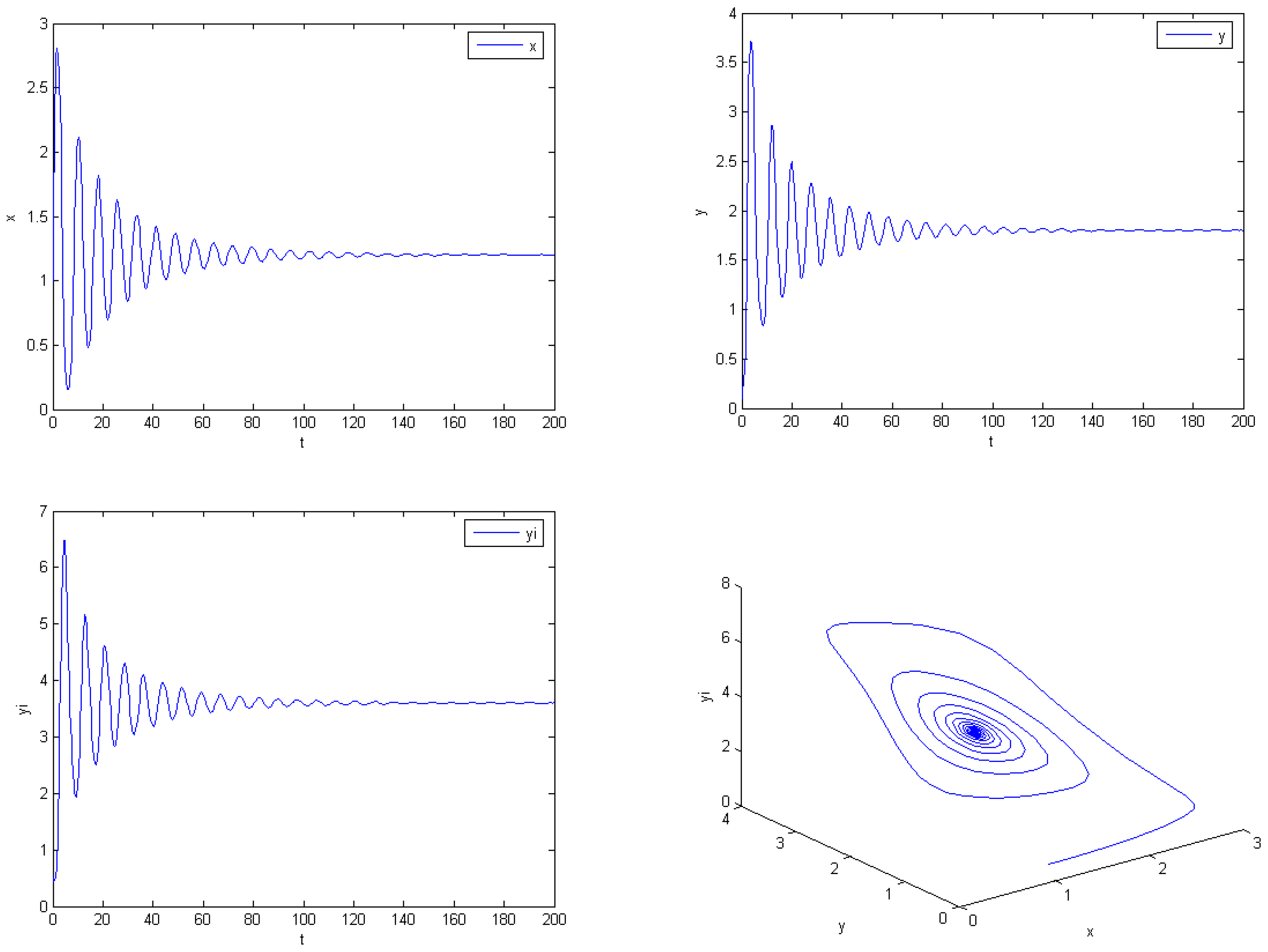
(i) $\tau =1.2,$ $\tau <{\tau }_0$. In this case, the numerical simulation (see Figure 1) shows that the predator and prey populations spiral toward the equilibrium $E^{*}(1.2,1.8,3.6)$;

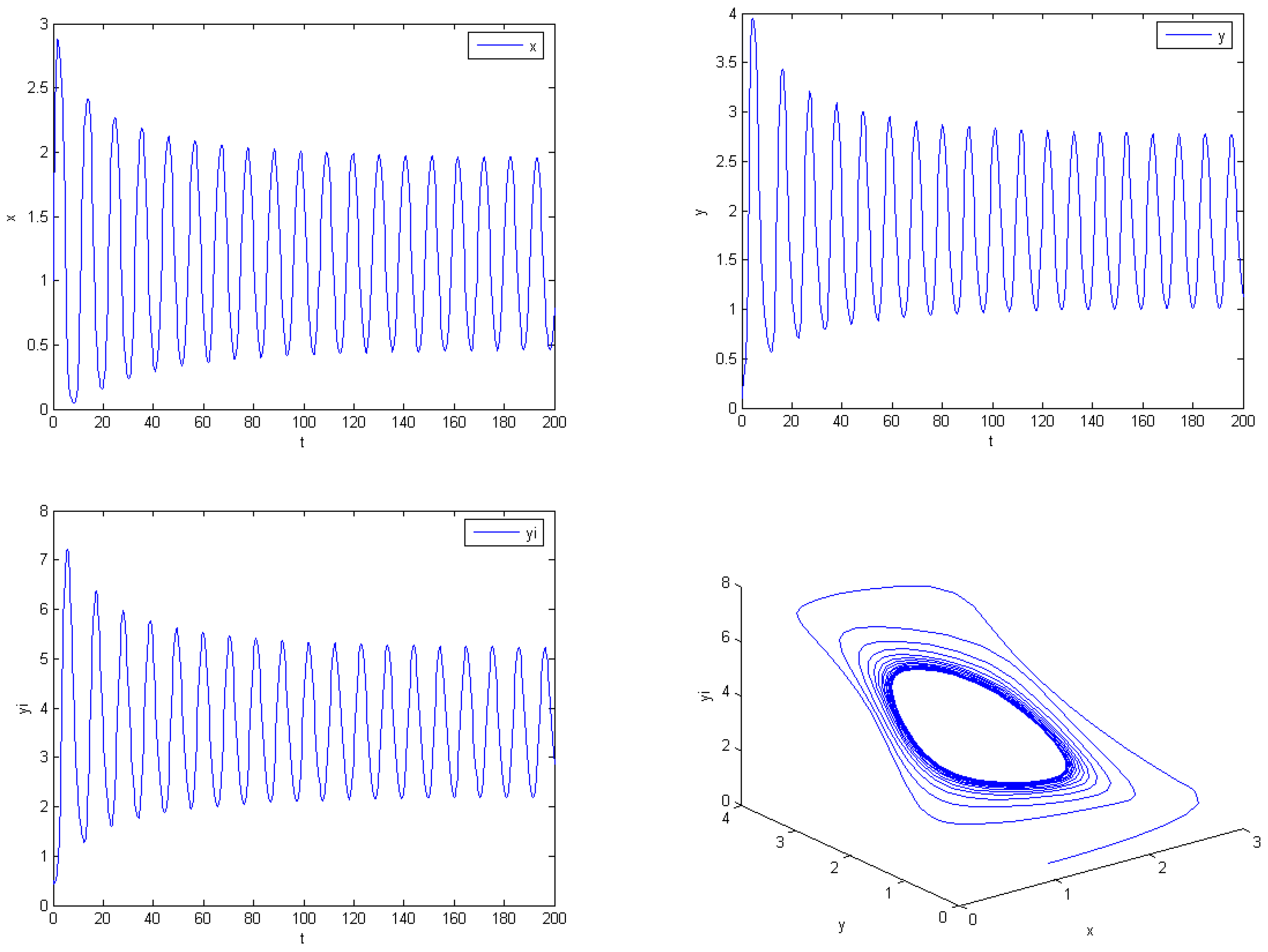
(ii) By calculation, we obtain ${\tau }_0=1.3434655328.$ By Theorem 5.1, a Hopf bifurcation occurs when $\tau ={\tau }_0$. Select $\tau =1.8$. From Figure 2, we can find that both the predator and prey populations reach periodic oscillations around the equilibrium $E^{*}(x^{*},y^{*},y_i^{*})$ in finite time;

(iii) From our calculations, we can see that ${\omega }_0=0.6514262661$ and ${\lambda }^{\prime }({\tau }_0)=0.6127495603$ $+0.4261524984i$. From the formulae (50), we can obtain $c_1(0)=-10.29371206-73.4416490i,$ ${\mu }_2>0,$${\beta }_2<0$ and $T_2>0$. Hence, the Hopf bifurcation is supercritical, the direction of the bifurcation is $\tau >{\tau }_0$ and these bifurcating periodic solutions are stable (see Figure 2).

8. Discussion

In this paper, a new dynamics for a predator–prey model with staged structure and time delay has been analyzed. We discuss the influence of the parameter $\tau$ on the dynamics of the system (3). The system (3) is permanent under some conditions. The local and global stability of the positive equilibrium is presented. By choosing $\tau$ as a bifurcation parameter, we prove that the delay loss of stability phenomenon appears under the conditions $1-\alpha \beta <0$ and $q^2-2ps-l^2>0$. That is to say, there is a critical value ${\tau }_0$ of $\tau$ such that system (3) is stable in the range $\tau \in (0,{\tau }_0)$ at positive equilibrium $E^{*}$ (see Figure 1); when $\tau ={\tau }_0$, a Hopf bifurcation occurs around $E^{*}(x^{*},y^{*},y_i^{*})$; when $\tau >{\tau }_0$, the system is unstable (see Figure 2) and there are always Hopf bifurcations near the positive equilibrium $E^{*}(x^{*},y^{*},y_i^{*})$ when $\tau$ takes other critical values. We derive explicit formulae for determining the properties of Hopf bifurcation at the critical value of ${\tau }_0$ via the ideas of Hassard et al. If we do not consider the staged structure of the predator, system (2) has no periodic solutions, which shows that the staged structure of the predator can severely affect the dynamical behavior of the system. However, for system (3), there is no chaotic behavior of the system (3) by numerical simulations.

References

- Conejero, J.A.; Murillo-Arcila, M.; Seoane, J.M.; Seoane-Sepúlveda, J.B. When Does Chaos Appear While Driving? Learning Dynamical Systems via Car-Following Models. Math. Mag. 2022, 95, 302–313. [Google Scholar] [CrossRef]
- Zhou, X.; Shi, X.; Wei, M. Dynamical behavior and optimal control of a stochastic mathe-matical model for cholera. Chaos Solitons Fractals 2022, 156, 111854. [Google Scholar] [CrossRef]
- Owolabi, K.M. Computational dynamics of predator–prey model with the power-law k-ernel. Results Phys. 2021, 21, 103810. [Google Scholar] [CrossRef]
- Cao, Y.; Alamri, S.; Rajhi, A.A.; Anqi, A.E.; Riaz, M.B.; Elagan, S.K.; Jawa, T.M. A novel piece-wise approach to modeling interactions in a food web model Author links open overlay panel. Results Phys. 2021, 31, 104951. [Google Scholar] [CrossRef]
- Das, B.K.; Sahoo, D.; Samanta, G.P. Impact of fear in a delay-induced predator–prey system with intraspecific competition within predator species. Math. Comput. Simul. 2022, 191, 134–156. [Google Scholar] [CrossRef]
- Liu, Q.; Jiang, D.; Hayat, T. Dynamics of stochastic predator-prey models with distributed delay and stage structure for prey. Int. J. Biomath. 2021, 14, 2150020. [Google Scholar] [CrossRef]
- Alsakaji, H.J.; Kundu, S.; Rihan, F.A. Delay differential model of one-predator two-prey system with Monod-Haldane and holling type II functional responses. Appl. Math. Comput. 2021, 397, 125919. [Google Scholar] [CrossRef]
- Yousef, F.; Semmar, B.; Al Nasr, K. Dynamics and simulations of discretized Caputo-conformable fractional-order Lotka-Volterra models. Nonlinear Eng. 2022, 11, 100–111. [Google Scholar] [CrossRef]
- Yousef, F.; Semmar, B.; Al Nasr, K. Incommensurate conformable-type three-dimensional Lotka–Volterra model: Discretization, stability, and bifurcation. Arab. J. Basic Appl. Sci. 2022, 29, 113–120. [Google Scholar] [CrossRef]
- Chen, L.S.; Song, X.Y.; Lu, Z.Y. Mathematica Models and Methods in Ecology; Sichuan Science and Technology: Chengdu, China, 2003. (In Chinese) [Google Scholar]
- He, X.Z. The Lyapunov functionals for delay Lotka Volterra type models. SIAM J. Appl. Math. 1998, 58, 1222–1236. [Google Scholar] [CrossRef]
- Gopalsamy, K.; He, X.Z. Global stability in n-species competition modelled by “pure-delay type” systems II: Nonautonomous case. Can. Appl. Math. Q. 1998, 6, 17–43. [Google Scholar]
- He, X.Z. Global stability in nonautonomous Lotka–Volterra systems of “pure-delay type”. Differ. Integral Equations 1998, 11, 293–310. [Google Scholar]
- Wang, W.D.; Ma, Z.E. Harmless delays for uniform peristence. J. Math. Anal. Appl. 1991, 158, 256–268. [Google Scholar]
- Cui, J.A.; Chen, L.S.; Wang, W.D. The effect of dispersal on population growth with stage- structure. Comput. Appl. Math. 2000, 39, 91–102. [Google Scholar] [CrossRef] [Green Version]
- Song, X.Y.; Cui, J.A. The Stage-structured predator–prey System with Delay and Harvesting. Appl. Anal. 2002, 81, 1127–1142. [Google Scholar] [CrossRef]
- Aiello, W.G.; Freedman, H. A time-delay model of single-species growth with stage structure. Math. Biosci. 1990, 101, 139–153. [Google Scholar] [CrossRef]
- Cao, Y.; Fan, J.; Gard, T.C. The effects of state-dependent time delay on a stage-structured population growth model. Nonlinear Anal. Theory Methods Appl. 1992, 19, 95–105. [Google Scholar] [CrossRef]
- Walter, W. Ordinary Differential Equations. Graduate Texts in Mathematics; Springer: Now York, NY, USA, 1998; Volume 18. [Google Scholar]
- Hale, J.K.; Waltman, P. Persistence in inffnite-dimensional systems. SIAM J. Math. Anal. 1989, 20, 388–396. [Google Scholar] [CrossRef]
- Kuang, Y. Delay Differential Equations with Applications in Population Dynamics; Academic Press: London, UK, 2004. [Google Scholar]
- Hassard, B.D.; Kazarini, N.D.; Wan, Y.H. Theory and Application of Hopf Bifurcation; London Mathematical Society Lecture Note Series, 41; Cambridge University Press: Cambridge, UK, 1981. [Google Scholar]
Figure 1.
, , , , , , , . The solution tends to the positive equilibrium. The initial value is constant function for .
Figure 2.
Trajectory of the system with same parameters as Figure 1. except that . The solution tends to the periodic solution. The initial value is constant function for .
Publisher’s Note: MDPI stays neutral with regard to jurisdictional claims in published maps and institutional affiliations. |
© 2022 by the author. Licensee MDPI, Basel, Switzerland. This article is an open access article distributed under the terms and conditions of the Creative Commons Attribution (CC BY) license (https://creativecommons.org/licenses/by/4.0/).
Share and Cite
MDPI and ACS Style
Zhou, X. Stability and Hopf Bifurcation Analysis of a Stage-Structured Predator–Prey Model with Delay. Axioms 2022, 11, 575. https://doi.org/10.3390/axioms11100575
AMA Style
Zhou X. Stability and Hopf Bifurcation Analysis of a Stage-Structured Predator–Prey Model with Delay. Axioms. 2022; 11(10):575. https://doi.org/10.3390/axioms11100575
Chicago/Turabian StyleZhou, Xueyong. 2022. "Stability and Hopf Bifurcation Analysis of a Stage-Structured Predator–Prey Model with Delay" Axioms 11, no. 10: 575. https://doi.org/10.3390/axioms11100575
Note that from the first issue of 2016, this journal uses article numbers instead of page numbers. See further details here.