Article

A Reliable Technique for Solving Fractional Partial Differential Equation

1
Department of Mathematical Sciences, Faculty of Sciences, Princess Nourah Bint Abdulrahman University, P.O. Box 84428, Riyadh 11671, Saudi Arabia
2
Department of Mathematics, Abdul Wali Khan University, Mardan 23200, Pakistan
3
Department of Mechanical Engineering, Sejong University, Seoul 05006, Korea
4
FRESLIPS, University College Dublin, D4 Dublin, Ireland
*
Author to whom correspondence should be addressed.
These authors contributed equally to this work and are co-first authors.
Axioms 2022, 11(10), 574; https://doi.org/10.3390/axioms11100574
Submission received: 27 September 2022 / Revised: 10 October 2022 / Accepted: 14 October 2022 / Published: 20 October 2022
(This article belongs to the Special Issue Mathematical Modeling with Differential Equations)

Abstract

:
The development of numeric-analytic solutions and the construction of fractional-order mathematical models for practical issues are of the greatest importance in a variety of applied mathematics, physics, and engineering problems. The Laplace residual-power-series method (LRPSM), a new and dependable technique for resolving fractional partial differential equations, is introduced in this study. The residual-power-series method (RPSM), a well-known technique, and the Laplace transform (LT) are elegantly combined in the suggested technique. This innovative approach computes the fractional derivative in the Caputo sense. The proposed method for handling fractional partial differential equations is provided in detail, along with its implementation. The novel approach yields a series solution to fractional partial differential equations. To validate the simplicity, effectiveness, and viability of the suggested technique, the provided model is tested and simulated. A numerical and graphical description of the effects of the fractional order γ on approximating the solutions is provided. Comparative results show that the suggested method approximates more precisely than current methods such as the natural homotopy perturbation method. The study showed that the aforementioned method is straightforward, trustworthy, and suitable for analysing non-linear engineering and physical issues.

1. Introduction

It has been noted that fractional-order α derivatives, often in the range between 0 and 1, are a helpful tool for describing a variety of events [1]. To obtain the desired order of a fractional derivative, the Caputo fractional derivative computes an ordinary derivative first, then a fractional integral. In reverse order, the Riemann–Liouville fractional derivative is calculated. As a result, although the Riemann–Liouville fractional derivative permits initial conditions in terms of fractional integrals and their derivatives, and the Caputo fractional derivative only enables the involvement of conventional initial and boundary conditions. These two operators coincide under the homogeneous initial condition assumption. Anyone who has studied fundamental calculus is familiar with the differentiation operator D = d d ς . Furthermore, provided that n is a positive integer, the nth derivative of u, denoted by D γ u ( ς ) = d n u ( ς ) d ς n , is well defined for suitable functions u. L’Hôpital asked Leibnitz in 1695 what significance could be assigned to D n u ( ς ) if n were a fraction. However, it was not until 1884 that the theory of generalized operators reached a stage in its evolution that was appropriate for the modern mathematician to use as a starting point. By that time, the theory had been expanded to include operators D v , where m could be real or complex, rational or irrational, and positive or negative [2]. Although derivatives of arbitrary order were discussed by Leibniz, Euler, Laplace, Lacroix, and Fourier, Niels Henrik Abel used fractional operations for the first time in 1823. In order to solve the tautochrone paradox, Abel used fractional calculus [2]. Liouville is to be credited with making what is likely the first sincere attempt to define a fractional derivative logically. He wrote nine articles on the topic between 1832 and 1837, with the latest one in the field appearing in 1855. In recent years, it has been discovered that the fractional calculus is very effective in describing a wide variety of physical phenomena, including damping laws and diffusion processes [2,3,4,5]. Kilbas and Trujillo [1], Caputo [6], Debanth [7], Jafari and Seifi [8], Kemple and Beyer [9], Oldham and Spanier [10], Momani and Shawagfeh [11], and others provide some fundamental works on various elements of the fractional calculus [12,13,14,15,16].
Over the past forty years, fundamental research and advancements on fractional derivatives and differential equations have been made. Traditional differential equations with non-local and genetic significance in material characteristics are generalized as fractional-order differential equations. Fractional partial differential equations are increasingly used in the creation of non-linear models and the analysis of dynamical systems. The theory of fractional-order calculus has been connected to real-world projects and used to examine and investigate a variety of phenomena, such as chaos theory [17], financial models [18], a noisy environment [19], optics [20], and others [21,22,23,24]. The characteristics of non-linear issues that occur in nature are largely described by the solutions of fractional differential equations. Since it is challenging to find an accurate solution for fractional differential equations representing non-linear phenomena, many analytical and numerical techniques are employed [25,26,27,28].
In recent years, scholars and researchers have paid close attention to both the numerical and analytical solutions of PDE systems. For resolving fractional FPDEs such as this, numerous numerical and analytical algorithms have been used, including the first integral method [29], the Elzaki transform decomposition method [30,31], the double Laplace transform method [32], the homotopy perturbation transform method [33,34], the conformable fractional Laplace transform method [35], the Yang transform decomposition method [36,37], the generalized two-dimensional differential transform method [38], the Fourier transform [39], He’s variational iteration method [40], the fractional complex differential transformation method [41], and the fractional variational iteration method [42].
The power-series method (PSM), which results in a closed-form solution of known functions, is well proven as an efficient method for solving linear ordinary-partial differential equations. In the case of nonlinear problems, it is impossible to obtain a closed-form solution, and finding out the series coefficients is a highly challenging task. A modified version of the PSM that treats the coefficients as transformed functions that follow a set of rules and are determined in recurrence relations is introduced to address the aforementioned limitations of the standard PSM. The differential transform method is the name of this improvement (DTM). Different kinds of integro-differential equations and linear-nonlinear equations have both been solved using it. Another advancement is the establishment of the residual-power-series method (RPSM) through the differentiation of the nth ordered coefficient of the PSM’s nth partial sum of the PSM (n-1)-times.
It was necessary to increase the use of the power-series method to deal with fractional difficulties during the modification of the ordinary derivative to a fractional derivative because it is more general. Many significant models that arise in various branches of science and engineering are constructed and solved analytically using the fractional DTM and fractional RPS methodologies. By including the Laplace transform (LT) into the RPSM’s technique, we hope to improve its accuracy in this work. This RPSM promotion is known as the Laplace residual-power-series method (LRPSM). Solving the FPDEs introduces the building of this innovative approach. Accuracy to the necessary level has been attained. The suggested technique has a very easy and uncomplicated process. The findings indicate that, in comparison to other analytical procedures, the current method has the appropriate accuracy.
The framework of the study is detailed as follows. First, we use key FC theory ideas and findings in Section 2. Additionally, several original findings that provide the basis for the innovative technique in Section 2 are provided. The solutions to time-fractional PDEs are then determined in Section 3 using the LRPSM. Some of the problems in Section 4 are solved using LRPSM. A brief conclusion ends Section 6.

2. Preliminaries

Here, we provide some definitions in terms of Caputo and Riemann–Liouville, along with the Laplace transform theorem.
Definition 1.
The fractional derivative in terms of Caputo is stated as [6,43]
C D η γ u ( ς , η ) = J η m γ u m ( ς , η ) , m 1 < γ m , η > 0 ,
where m N and J η γ represents a fractional integral in terms of Riemann–Liouville (RL) as
J η γ u ( ς , η ) = 1 Γ ( γ ) 0 η ( η t ) γ 1 u ( ς , t ) d t .
Definition 2.
The LT is stated as [43]
u ( ς , μ ) = L η [ u ( ς , η ) ] = 0 e μ η u ( ς , η ) d η , μ > γ ,
with inverse LT as
u ( ς , η ) = L η 1 [ u ( ς , μ ) ] = l i l + i e μ η u ( ς , μ ) d μ , l = R e ( μ ) > l 0 .
Lemma 1.
Suppose u ( ς , η ) is a piecewise continuous function with U ( ς , μ ) = L η [ u ( ς , η ) ] , so
1.
L η [ J η γ u ( ς , η ) ] = U ( ς , μ ) μ γ , γ > 0 .
2.
L η [ D η γ u ( ς , η ) ] = μ γ U ( ς , μ ) k = 0 m 1 μ γ k 1 u k ( ς , 0 ) , m 1 < γ m .
3.
L η [ D η n γ u ( ς , η ) ] = μ n γ U ( ς , μ ) k = 0 n 1 μ ( n k ) γ 1 D η k γ u ( ς , 0 ) , 0 < γ 1 .
Proof. 
For proof, see [44]. □
Theorem 1.
Let us assume that u ( ς , η ) is a continuous piecewise on I × [ 0 , ) and that ϑ is the order of the exponential function. Take the function U ( ς , μ ) = L η [ u ( ς , η ) ] with fractional expansion as
U ( ς , μ ) = n = 0 f n ( ς ) μ 1 + n γ , 0 < γ 1 , ς I , μ > ϑ .
So, f n ( ς ) = D η n γ u ( ς , 0 ) .
Proof. 
For proof, see [43]. □
Remark 1.
On taking the inverse LT of Equation (5) as provided in [43]:
u ( ς , η ) = i = 0 D η γ u ( ς , 0 ) Γ ( 1 + i γ ) η i ( ϑ ) , 0 < ϑ 1 , η 0 .
This corresponds to the fractional Taylor’s formula described in [45].
The convergence of the FPS in Theorem (1) is explained and proven by the following theorem.

3. General Methodology of LRPSM

D η γ u ( ς , η ) = c D ς 2 u ( ς , η ) + a u ( ς , η ) b u 4 ( ς , η ) , 1 < γ 2 ,
with initial source
u ( ς , 0 ) = f 0 ( ς ) , u η ( ς , 0 ) = g 0 ( ς ) .
By employing LT to (7),
L D μ γ u ( ς , η ) = c L D ς 2 u ( ς , η ) + a L 2 [ u ( ς , η ) ] b L u 4 ( ς , η ) .
As from the fact that C D 1 a w ( ς , η ) = μ a L [ w ( ς , η ) ] μ a 1 u ( ς , 0 ) μ a 2 u ( ς , 0 ) and by utilizing the initial condition (8), we have
U ( ς , μ ) = f 0 ( ς ) + g 0 ( ς ) μ + c μ a D μ 2 U ( ς , μ ) + a μ a U ( ς , μ ) b μ a L 2 C 1 [ U ( ς , μ ) ] a ,
with U ( ς , μ ) = L [ w ( ς , η ) ] .
We may express the transformed function U ( ς , μ ) in the following manner:
U ( ς , μ ) = n = 0 f μ ( ς ) μ n γ + 1 .
The kth-truncated series of (11) can be expressed as
U k ( ς , μ ) = n = 0 k f μ ( ς ) μ n γ + 1 = f o ( ς ) + g 0 ( ς ) μ + n = 1 k f k ( ς ) μ n γ + 1 .
As provided in [46], from the definition of the Laplace residual function
L R e s k ( ς , μ ) = U k ( ς , μ ) f 0 ( ς ) + g 0 ( ς ) μ c μ γ D μ 2 U k ( ς , μ ) a μ γ U k ( ς , μ ) + b μ γ L L 1 [ U k ( ς , μ ) ] q .
We provide several features that emerge in the common residual power series approach [46]:
  • L Res ( ς , μ ) = 0 and lim k L Res μ k ( ς , μ ) = L Res ( ς , μ ) for each μ > 0 .
  • lim μ μ L Res ( ς , μ ) = 0 lim μ μ L Res ( ς , μ ) = 0 .
  • lim μ μ k γ + 1 L Res ( ς , μ ) = lim μ μ k γ + 1 L Res k ( ς , μ ) = 0 , 0 < γ 1 , k = 1 , 2 , 3 , We will now solve the system below recursively in order to define the coefficient functions f n ( ς ) .
lim μ μ k a + 1 L R e s k ( ς , μ ) = 0 , 0 < γ 1 , k = 1 , 2 , 3 ,
The next step is to take the inverse LT of U k ( ς , μ ) to obtain the kth approximation u k ( ς , η ) .

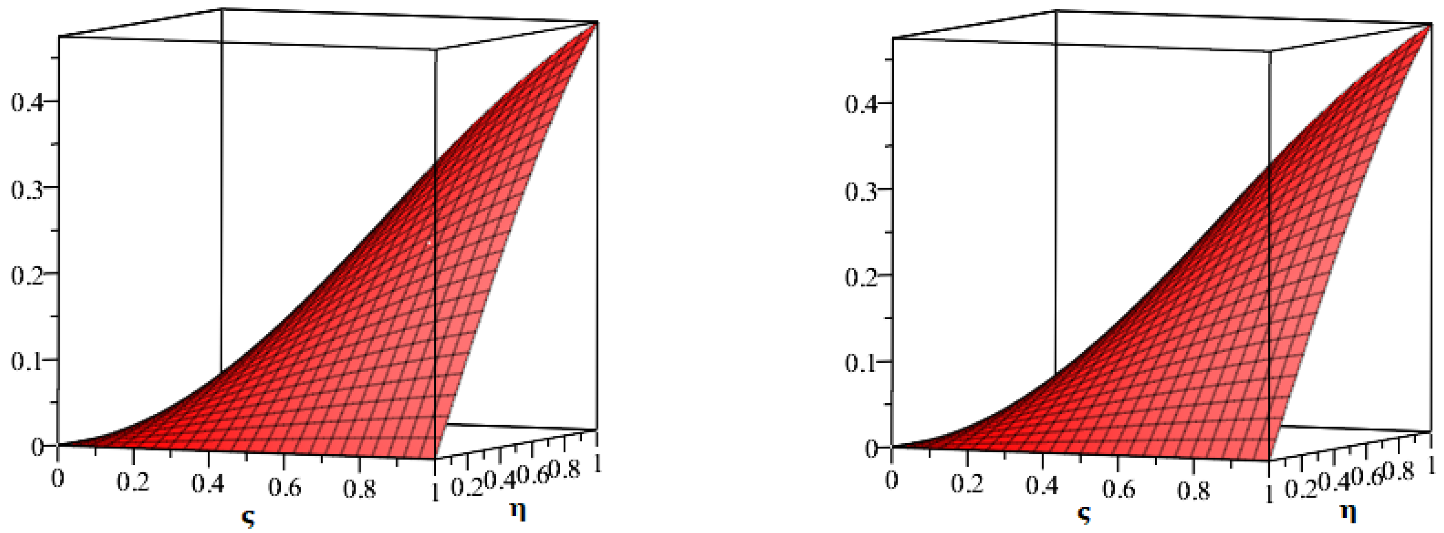
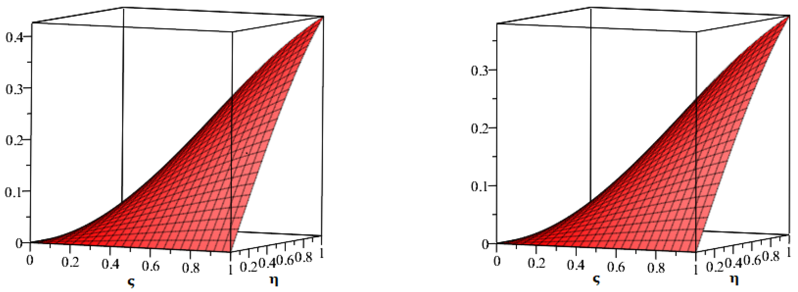
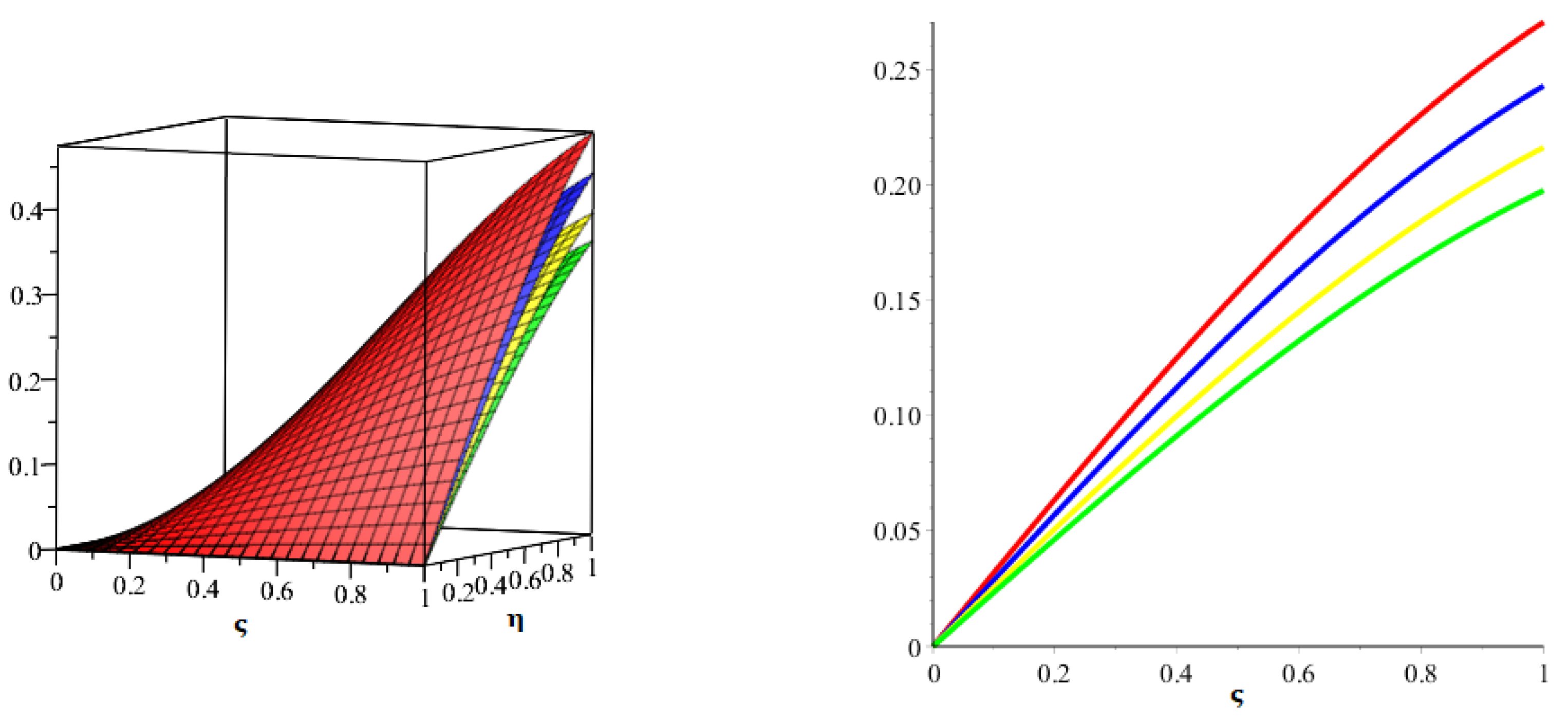
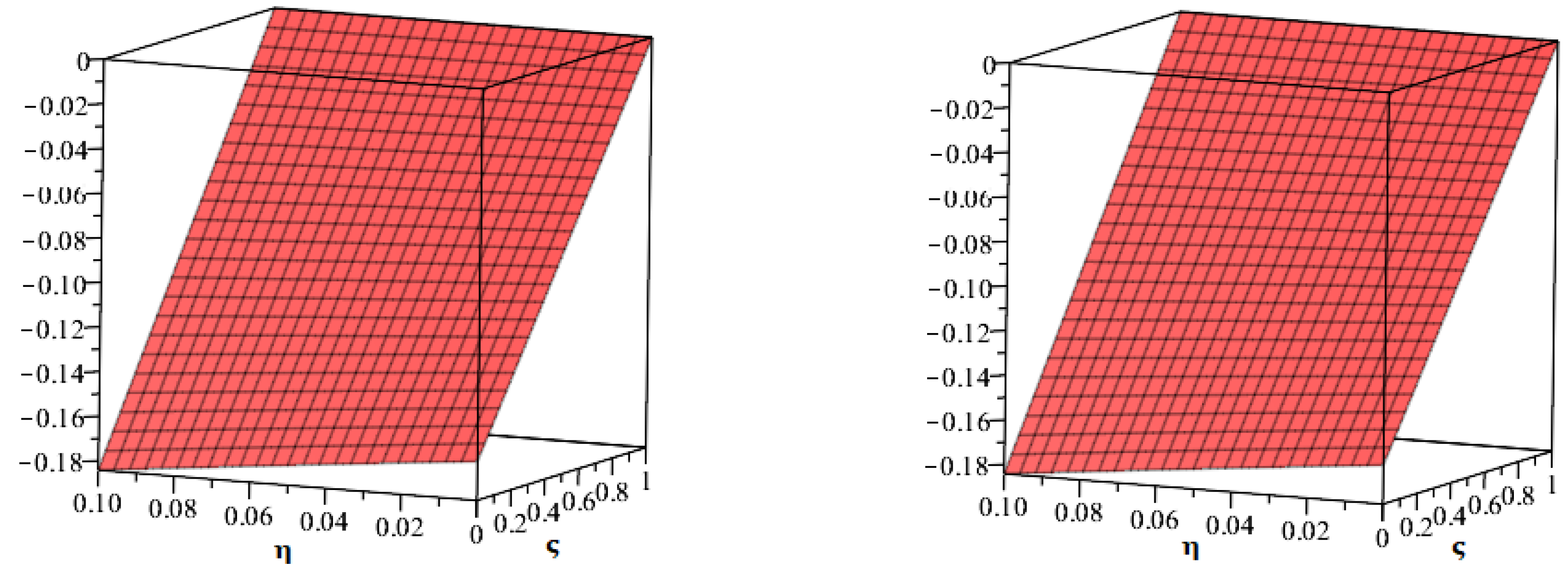
4. Numerical Examples

Here, we solve three problems to show the accuracy of the proposed method.

4.1. Problem

Assume the fractional partial differential equation of the following form:
D η γ u u ς ς 2 u = 0 , 1 < γ 2 ,
with the initial condition
u ( ς , , 0 ) = sin ( ς ) sin ( ) , u η ( ς , , 0 ) = 0 .
By employing LT to Equation (1) and by using Equation (9), we obtain
U ( ς , , μ ) sin ( ς ) sin ( ) μ + 1 μ γ L η L η 1 [ U ς ς ] + L η 1 [ U ] = 0 .
The kth-truncated series can be expressed as
U ( ς , μ ) = sin ( ς ) sin ( ) μ + n = 1 k f n ( ς , , μ ) μ n γ + 1 , k = 1 , 2 , 3 , 4
so the kth-LRFs are
L t R e s u , k ( ς , , μ ) = U k ( ς , , μ ) sin ( ς ) sin ( ) μ + 1 μ γ L η L η 1 [ U ς ς , k ] + L η 1 [ U , , k ] .
The kth-truncated series Equation (17) will be substituted into the kth-truncated residual function Equation (18) to yield f k ( ς , , μ ) . The resulting equation, μ k γ + 1 , will then be multiplied, and the relation lim μ ( μ k γ + 1 L t R e s u , k ( ς , , μ ) ) = 0 , k = 1 , 2 , 3 , . Several terms are as
f 1 ( ς , , μ ) = ( 4 ) sin ( ς ) sin ( ) , f 2 ( ς , , μ ) = ( 4 ) 2 sin ( ς ) sin ( ) , f 3 ( ς , , μ ) = ( 4 ) 3 sin ( ς ) sin ( ) , f 4 ( ς , , μ ) = ( 4 ) 4 sin ( ς ) sin ( ) ,
and so on.
We may now obtain by altering the values of f k ( ς , μ ) , k = 1 , 2 , 3 , , in Equation (17).
U ( ς , , μ ) = sin ( ς ) sin ( ) μ + ( 4 ) sin ( ς ) sin ( ) μ γ + 1 + ( 4 ) 2 sin ( ς ) sin ( ) μ 2 γ + 1 + ( 4 ) 3 sin ( ς ) sin ( ) μ 3 γ + 1 + ( 4 ) 4 sin ( ς ) sin ( ) μ 4 γ + 1 + .
By employing inverse LT, we obtain
u ( ς , η ) = sin ( ς ) sin ( ) 4 sin ( ς ) sin ( ) η γ Γ ( γ + 1 ) + ( 4 ) 2 sin ( ς ) sin ( ) η 2 γ Γ ( 2 γ + 1 ) ( 4 ) 3 sin ( ς ) sin ( ) η 3 γ Γ ( 3 γ + 1 ) + ( 4 ) 4 sin ( ς ) sin ( ) η 4 γ Γ ( 4 γ + 1 ) + .
u ( ς , , η ) = sin ( ς ) sin ( ) 1 4 η γ Γ ( γ + 1 ) + ( 4 η γ ) 2 Γ ( 2 γ + 1 ) ( 4 η γ ) 3 Γ ( 3 γ + 1 ) + ( 4 η γ ) 4 Γ ( 4 γ + 1 ) + .
On putting γ = 1 , we have
u ( ς , , η ) = sin ( ς ) sin ( ) 1 4 η 1 ! + ( 4 η ) 2 2 ! ( 4 η ) 3 3 ! + ( 4 η ) 4 4 ! + , u ( ς , , η ) = sin ( ς ) sin ( ) e 4 η .

4.2. Problem

Assume the fractional partial differential equation of the following form:
D η γ u 6 u ς u + u ς ς ς = 0 , 0 < γ 1 ,
with the initial condition
u ( ς , 0 ) = 1 6 ( ς 1 ) .
By employing LT to Equation (23) and by using Equation (24), we obtain
U ( ς , μ ) 1 6 ( ς 1 ) μ 1 μ γ L η 6 L η 1 [ U ς ] L η 1 [ U ] L η 1 [ U ς ς ς ] = 0 .
The kth-truncated series can be expressed as
U ( ς , μ ) = 1 6 ( ς 1 ) μ + n = 1 k f n ( ς , μ ) μ n γ + 1 , k = 1 , 2 , 3 , 4
so the kth-LRFs are
L η R e s u , k ( ς , μ ) = U k ( ς , μ ) 1 6 ( ς 1 ) μ + 1 μ γ L η 6 L η 1 [ U ς , k ] L η 1 [ U k ] L η 1 [ U ς ς ς , k ] .
The kth-truncated series Equation (26) will be substituted into the kth-truncated residual function Equation (27) to yield f k ( ς , , μ ) . The resulting equation, μ k γ + 1 will then be multiplied, and the relation lim μ ( μ k γ + 1 L t R e s u , k ( ς , , μ ) ) = 0 , k = 1 , 2 , 3 , . Several terms are as
f 1 ( ς , μ ) = ( ς 1 ) 6 , f 2 ( ς , μ ) = ( ς 1 ) 6 , f 3 ( ς , μ ) = ( ς 1 ) 6 ,
and so on.
We may now obtain by altering the values of f k ( ς , μ ) , k = 1 , 2 , 3 , , in Equation (26).
U ( ς , μ ) = 1 6 ( ς 1 ) μ + ( ς 1 ) 6 μ γ + 1 + ( ς 1 ) 6 μ 2 γ + 1 + ( ς 1 ) 6 μ 3 γ + 1 + .
By employing inverse LT, we obtain
u ( ς , η ) = 1 6 ( ς 1 ) + ( ς 1 ) 6 η γ Γ ( γ + 1 ) + ( ς 1 ) 6 η 2 γ Γ ( 2 γ + 1 ) + ( ς 1 ) 6 η 3 γ Γ ( 3 γ + 1 ) + .
On putting γ = 1 , we have
u ( ς , η ) = 1 6 ς 1 1 η .

4.3. Problem

Assume the fractional partial differential equation of the following form:
D η γ u u 3 u ς u = 0 , 0 < γ 1 ,
with the initial condition
u ( ς , 0 ) = a 3 b 2 ς 2 3 .
By employing LT in Equation (31) and by using Equation (32), we obtain
U ( ς , μ ) a 3 b 2 ς 2 3 μ + 1 μ γ L η L η 1 [ U 3 ] L η 1 [ U ς ] L η 1 [ U ] = 0 .
The kth-truncated series can be expressed as
U ( ς , μ ) = a 3 b 2 ς 2 3 μ + n = 1 k f n ( ς , μ ) μ n γ + 1 , k = 1 , 2 , 3 , 4
so the kth-LRFs are
L η R e s u , k ( ς , μ ) = U k ( ς , μ ) a 3 b 2 ς 2 3 μ + 1 μ γ L η L η 1 [ U k 3 ] L η 1 [ U ς , k ] L η 1 [ U k ] .
The kth-truncated series Equation (34) will be substituted into the kth-truncated residual function Equation (35) to yield f k ( ς , , μ ) . The resulting equation, μ k γ + 1 , will then be multiplied, and the relation lim μ ( μ k γ + 1 L t R e s u , k ( ς , , μ ) ) = 0 , k = 1 , 2 , 3 , . Several terms are as
f 1 ( ς , μ ) = b 2 3 a 3 b 2 ς 1 3 , f 2 ( ς , μ ) = b 3 2 a 3 b 2 ς 4 3 , f 3 ( ς , μ ) = b 9 2 a 3 b 2 ς 7 3 15 2 Γ ( 2 γ + 1 ) 2 ( Γ ( γ + 1 ) ) 2 16 ,
and so on.
We may now obtain by altering the values of f k ( ς , μ ) , k = 1 , 2 , 3 , , in Equation (34).
U ( ς , μ ) = a 3 b 2 ς 2 3 μ + b 2 3 a 3 b 2 ς 1 3 μ γ + 1 + b 3 2 a 3 b 2 ς 4 3 μ 2 γ + 1 + b 9 2 a 3 b 2 ς 7 3 15 2 Γ ( 2 γ + 1 ) 2 ( Γ ( γ + 1 ) ) 2 16 μ 3 γ + 1 + .
By employing inverse LT, we obtain
u ( ς , η ) = a 3 b 2 ς 2 3 b 2 3 a 3 b 2 ς 1 3 η γ Γ ( γ + 1 ) b 3 2 a 3 b 2 ς 4 3 η 2 γ Γ ( 2 γ + 1 ) + b 9 2 a 3 b 2 ς 7 3 15 2 Γ ( 2 γ + 1 ) 2 ( Γ ( γ + 1 ) ) 2 16 η 3 γ Γ ( 3 γ + 1 ) + .
On putting γ = 1 , we have
u ( ς , η ) = a 3 b 2 ( ς + b η ) 2 3 .

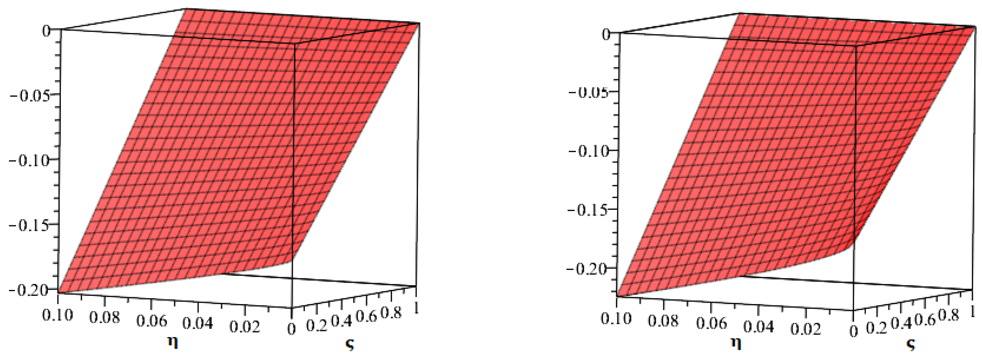
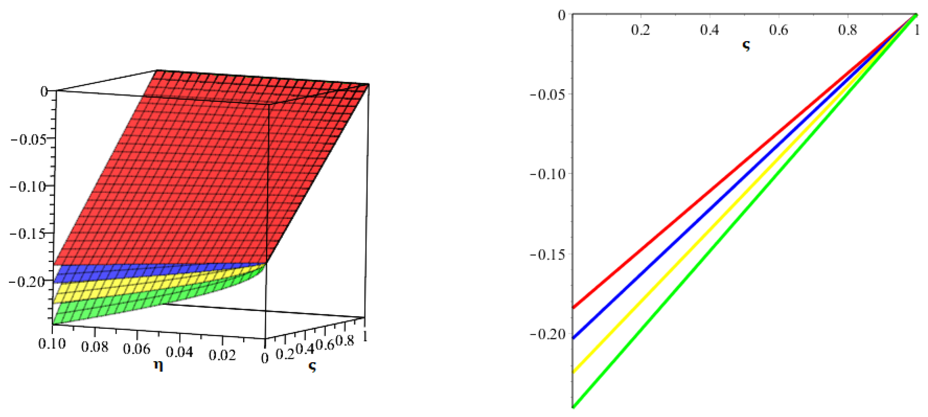
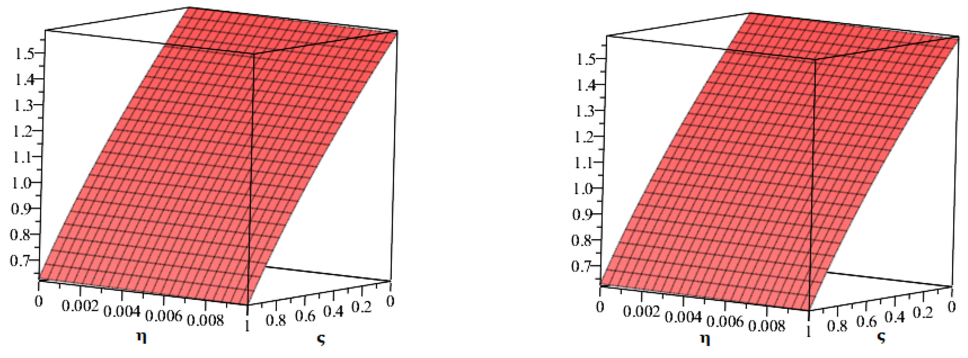
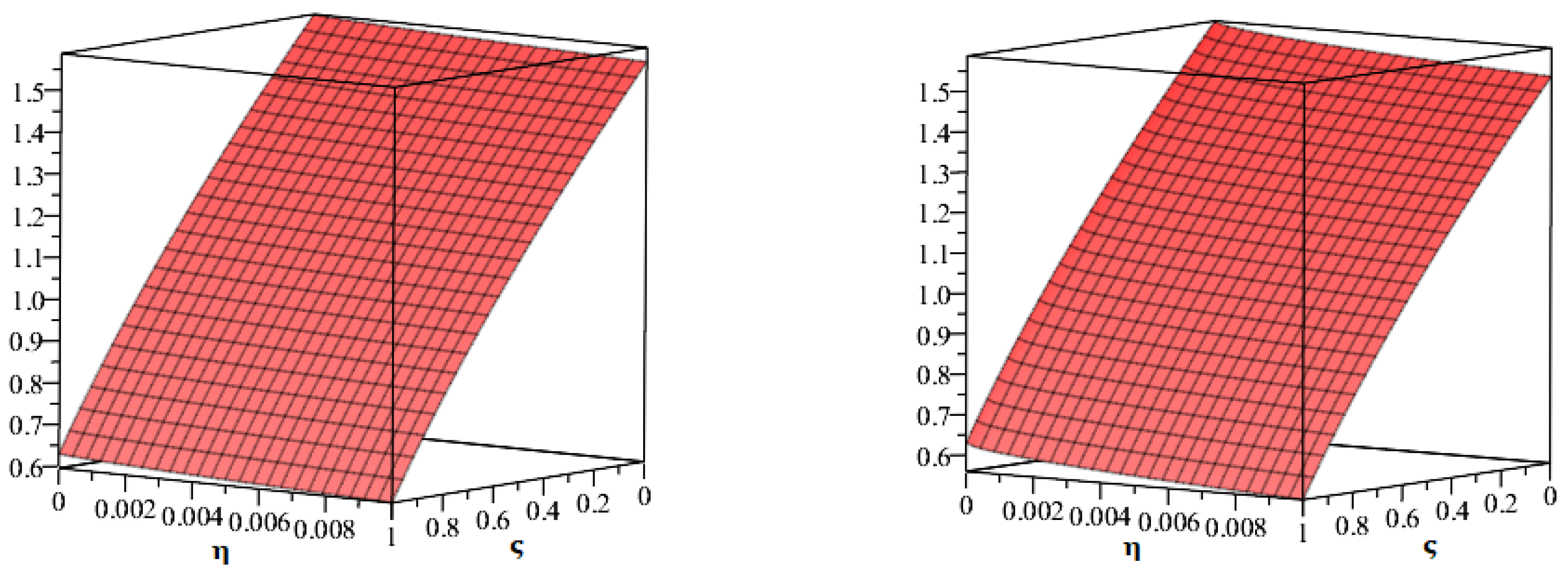
5. Results and Discussion

The numerical analysis between exact and approximative solutions, as shown in Table 1, Table 2 and Table 3, has been investigated in detail and with more precision in this study. The correctness and simplicity of the suggested method are demonstrated by computing the numerical values at different fractional orders. Table 1, Table 2 and Table 3 display the numerical comparison of the accurate and approximative solutions, demonstrating that the series solution soon converges to a small value. As a result, adding more terms for an approximate solution increases the accuracy of the analytical result. Figure 1 shows how the accurate and suggested approaches behave, as well as the characteristics of the approximative solution. For a better understanding of the problem’s characteristics, we also provide the suggested method solution at various fractional orders in Figure 2 and Figure 3. Figure 4 calculates the solution to problem 2 using the suggested and actual method. Figure 5 displays the graphical representations for γ = 0.8 , 0.6 . The behaviour of problem 2 in 2D and 3D for different fractional orders is shown in Figure 6. Similarly, Figure 7 presents the actual and suggested methods’ solutions at γ = 1 , whereas Figure 8 and Figure 9 present the proposed approach solution at different fractional orders. Based on the tables and graphs, we came to the conclusion that the proposed technique solution was in good agreement with the precise solution.

6. Conclusions

In this study, the Laplace residual-power-series method (LRPSM), a powerful new technique for solving fractional partial differential equations, is developed by successfully combining the residual-power-series method (RPSM) and the Laplace transform. The new technique provides a series solution with elegant computational terms that quickly converges to an exact or approximate solution. The fractional derivative is handled in the Caputo sense in this novel analytical technique. With the help of the new analytical technique, fractional partial differential equations are successfully solved precisely. The obtained results via our technique are compatible with the results obtained by the natural homotopy perturbation method. In order to understand the behavior of the provided problems, solutions at different fractional orders are taken and are shown with the help of graphs and tables, which confirm that we get closer to the exact solution as the order of γ goes from fractional-order towards the integercorder. It is clearly proven that the new reliable approach is both straightforward and highly accurate. The Laplace residual-power-series method is a powerful and reliable technique for handling fractional partial differential equations that are both linear and nonlinear.

Author Contributions

Conceptualization, A.S.A. and I.D.; methodology, R.S.; software, N.A.S.; validation, R.S.; formal analysis, I.D.; investigation, R.S.; resources, N.A.S.; data curation, I.D.; writing—original draft preparation, R.S.; writing—review and editing, N.A.S.; visualization, A.S.A.; supervision, I.D.; project administration, N.A.S.; funding acquisition, I.D. All authors have read and agreed to the published version of the manuscript.

Funding

This work was supported by Princess Nourah bint Abdulrahman University Researchers Supporting Project number (PNURSP2022R183), Princess Nourah bint Abdulrahman University, P.O. Box 84428, Riyadh 11671, Saudi Arabia. This work was supported by Sustainable Energy Authority of Ireland (SEAI), with funding by Ioannis Dassios under Grant No. RDD/00681.

Institutional Review Board Statement

Not applicable.

Informed Consent Statement

Not applicable.

Data Availability Statement

Not applicable.

Acknowledgments

This work was supported by Princess Nourah bint Abdulrahman University Researchers Supporting Project number (PNURSP2022R183), Princess Nourah bint Abdulrahman University, P.O. Box 84428, Riyadh 11671, Saudi Arabia. This work was supported by Sustainable Energy Authority of Ireland (SEAI), with funding by Ioannis Dassios under Grant No. RDD/00681.

Conflicts of Interest

The authors declare no conflict of interest.

References

  1. Kilbas, A.A.; Srivastava, H.M.; Trujillo, J.J. Theory and Applications of Fractional Differential Equations; North-Holland Mathematics Studies; Elsevier: Amsterdam, The Netherlands, 2006. [Google Scholar]
  2. Miller, K.S.; Ross, B. An Introduction to the Fractional Calculus and Fractional Differential Equations; Wiley: New York, NY, USA, 1993. [Google Scholar]
  3. Ablowitz, M.J.; Clarkson, P.A. Solitons, Nonlinear Evolution Equations and Inverse Scattering; Cambridge University Press: New York, NY, USA, 1991. [Google Scholar]
  4. Podlubny, I. Fractional Differential Equations: An Introduction to Fractional Derivatives, Fractional Differential Equations, to Methods of Their Solution and Some of Their Applications; Academic Press: New York, NY, USA, 1999. [Google Scholar]
  5. Samko, S.G.; Kilbas, A.A.; Marichev, O.I. Fractional Integrals and Derivatives: Theory and Applications; Gordon and Breach: Yverdon, Switzerland, 1993. [Google Scholar]
  6. Caputo, M. Linear models of dissipation whose Q is almost frequency independent-II. Geophys. J. Int. 1967, 13, 529–539. [Google Scholar] [CrossRef]
  7. Debnath, L. Recent applications of fractional calculus to science and engineering. Int. J. Math. Math. Sci. 2003, 2003, 3413–3442. [Google Scholar] [CrossRef] [Green Version]
  8. Jafari, H.; Seifi, S. Solving a system of nonlinear fractional partial differential equations using homotopy analysis method. Commun. Nonlinear Sci. Numer. Simul. 2009, 14, 1962–1969. [Google Scholar] [CrossRef]
  9. Kemple, S.; Beyer, H. Global and Causal Solutions of Fractional Differential Equations. In Proceedings of the 2nd International Workshop on Transform Methods and Special Functions (SCTP), Varna, Bulgaria, 23–30 August 1996; p. 210. [Google Scholar]
  10. Oldham, K.B.; Spanier, J. The fractional calculus, academic press, new york. In The Fractional Calculus; Academic Press: New York, NY, USA, 1974. [Google Scholar]
  11. Momani, S.; Shawagfeh, N. Decomposition method for solving fractional Riccati differential equations. Appl. Math. Comput. 2006, 182, 1083–1092. [Google Scholar] [CrossRef]
  12. Zhang, L.; Rahman, M.U.; Ahmad, S.; Riaz, M.B.; Jarad, F. Dynamics of fractional order delay model of coronavirus disease. AIMS Math. 2022, 7, 4211–4232. [Google Scholar] [CrossRef]
  13. Shen, W.Y.; Chu, Y.M.; ur Rahman, M.; Mahariq, I.; Zeb, A. Mathematical analysis of HBV and HCV co-infection model under nonsingular fractional order derivative. Results Phys. 2021, 28, 104582. [Google Scholar] [CrossRef]
  14. Zhang, L.; ur Rahman, M.; Arfan, M.; Ali, A. Investigation of mathematical model of transmission co-infection TB in HIV community with a non-singular kernel. Results Phys. 2021, 28, 104559. [Google Scholar] [CrossRef]
  15. Rahman, M.U.; Ahmad, S.; Arfan, M.; Akgül, A.; Jarad, F. Fractional Order Mathematical Model of Serial Killing with Different Choices of Control Strategy. Fractal Fract. 2022, 6, 162. [Google Scholar] [CrossRef]
  16. Xu, C.; ur Rahman, M.; Baleanu, D. On fractional-order symmetric oscillator with offset-boosting control. Nonlinear Anal. Model. Control 2022, 27, 994–1008. [Google Scholar] [CrossRef]
  17. Baleanu, D.; Wu, G.-C.; Zeng, S.-D. Chaos analysis and asymptotic stability of generalized Caputo fractional differential equations. Chaos Solitons Fractals 2017, 102, 99–105. [Google Scholar] [CrossRef]
  18. Sweilam, N.H.; Hasan, M.M.A.; Baleanu, D. New studies for general fractional financial models of awareness and trial advertising decisions. Chaos Solitons Fractals 2017, 104, 772–784. [Google Scholar] [CrossRef]
  19. Liu, D.Y.; Gibaru, O.; Perruquetti, W.; Laleg-Kirati, T.M. Fractional order differentiation by integration and error analysis in noisy environment. IEEE Trans. Autom. Control 2015, 60, 2945–2960. [Google Scholar] [CrossRef]
  20. Esen, A.; Sulaiman, T.A.; Bulut, H.; Baskonus, H.M. Optical solitons to the space-time fractional (1+1)-dimensional coupled nonlinear Schrödinger equation. Optik 2018, 167, 150–156. [Google Scholar] [CrossRef]
  21. Veeresha, P.; Prakasha, D.G.; Baskonus, H.M. New numerical surfaces to the mathematical model of cancer chemotherapy effect in Caputo fractional derivatives. Chaos 2019, 29, 013119. [Google Scholar] [CrossRef]
  22. Shah, N.A.; Agarwal, P.; Chung, J.D.; El-Zahar, E.R.; Hamed, Y.S. Analysis of optical solitons for nonlinear Schrodinger equation with detuning term by iterative transform method. Symmetry 2020, 12, 1850. [Google Scholar] [CrossRef]
  23. Prakash, A.; Veeresha, P.; Prakasha, D.G.; Goyal, M. A homotopy technique for fractional order multi-dimensional telegraph equation via Laplace transform. Eur. Phys. J. Plus 2019, 134, 1–18. [Google Scholar] [CrossRef]
  24. Veeresha, P.; Prakasha, D.G.; Baskonus, H.M. Novel simulations to the time-fractional Fisher’s equation. Math. Sci. 2019, 13, 33–42. [Google Scholar] [CrossRef]
  25. Almutlak, S.A.; Weera, W.; El-Tantawy, S.A.; El-Sherif, L.S. Fractional View Analysis of Swift-Hohenberg Equations by an Analytical Method and Some Physical Applications. Fractal Fract. 2022, 6, 524. [Google Scholar] [CrossRef]
  26. Alshehry, A.S.; Imran, M.; Khan, A.; Weera, W. Fractional View Analysis of Kuramoto-Sivashinsky Equations with Non-Singular Kernel Operators. Symmetry 2022, 14, 1463. [Google Scholar] [CrossRef]
  27. Shah, N.A.; Hamed, Y.S.; Abualnaja, K.M.; Chung, J.D.; Shah, R.; Khan, A. A comparative analysis of fractional-order kaup-kupershmidt equation within different operators. Symmetry 2022, 14, 986. [Google Scholar] [CrossRef]
  28. Shah, N.A.; Alyousef, H.A.; El-Tantawy, S.A.; Shah, R.; Chung, J.D. Analytical Investigation of Fractional-Order Korteweg-De-Vries-Type Equations under Atangana-Baleanu-Caputo Operator: Modeling Nonlinear Waves in a Plasma and Fluid. Symmetry 2022, 14, 739. [Google Scholar] [CrossRef]
  29. Çenesiz, Y.; Baleanu, D.; Kurt, A.; Tasbozan, O. New exact solutions of Burgers’ type equations with conformable derivative. Waves Random Complex Media 2017, 27, 103–116. [Google Scholar] [CrossRef]
  30. Nonlaopon, K.; Alsharif, A.M.; Zidan, A.M.; Khan, A.; Hamed, Y.S.; Shah, R. Numerical investigation of fractional-order Swift-Hohenberg equations via a Novel transform. Symmetry 2021, 13, 1263. [Google Scholar] [CrossRef]
  31. Shah, N.A.; El-Zahar, E.R.; Akgül, A.; Khan, A.; Kafle, J. Analysis of Fractional-Order Regularized Long-Wave Models via a Novel Transform. J. Funct. Spaces 2022, 2022, 2754507. [Google Scholar] [CrossRef]
  32. Özkan, O.; Kurt, A. On conformable double Laplace transform. Opt. Quantum Electron. 2018, 50, 103. [Google Scholar] [CrossRef]
  33. Sunthrayuth, P.; Alyousef, H.A.; El-Tantawy, S.A.; Khan, A.; Wyal, N. Solving Fractional-Order Diffusion Equations in a Plasma and Fluids via a Novel Transform. J. Funct. Spaces 2022, 2022, 1899130. [Google Scholar] [CrossRef]
  34. Qin, Y.; Khan, A.; Ali, I.; Al Qurashi, M.; Khan, H.; Shah, R.; Baleanu, D. An efficient analytical approach for the solution of certain fractional-order dynamical systems. Energies 2020, 13, 2725. [Google Scholar] [CrossRef]
  35. Hashemi, M.S. Invariant subspaces admitted by fractional differential equations with conformable derivatives. Chaos Solitons Fractals 2018, 107, 161–169. [Google Scholar] [CrossRef]
  36. Zidan, A.M.; Khan, A.; Shah, R.; Alaoui, M.K.; Weera, W. Evaluation of time-fractional Fisher’s equations with the help of analytical methods. AIMS Math. 2022, 7, 18746–18766. [Google Scholar] [CrossRef]
  37. Alaoui, M.K.; Fayyaz, R.; Khan, A.; Shah, R.; Abdo, M.S. Analytical investigation of Noyes-Field model for time-fractional Belousov-Zhabotinsky reaction. Complexity 2021, 2021, 3248376. [Google Scholar] [CrossRef]
  38. Liu, J.; Hou, G. Numerical solutions of the space-and time-fractional coupled Burgers equations by generalized differential transform method. Appl. Math. Comput. 2011, 217, 7001–7008. [Google Scholar] [CrossRef]
  39. Sejdić, E.; Djurovixcx, I.; Stankovixcx, L. Fractional Fourier transform as a signal processing tool: An overview of recent developments. Signal Process. 2011, 91, 1351–1369. [Google Scholar] [CrossRef] [Green Version]
  40. Yusufoglu, E.; Bekir, A. Numerical simulations of the Boussinesq equation by He’s variational iteration method. Int. J. Comput. Math. 2009, 86, 676–683. [Google Scholar] [CrossRef]
  41. Özkan, O. Approximate analytical solutions of systems of fractional partial differential equations. Karaelmas Sci. Eng. J. 2017, 7, 63–67. [Google Scholar]
  42. Alderremy, A.A.; Aly, S.; Fayyaz, R.; Khan, A.; Shah, R.; Wyal, N. The Analysis of Fractional-Order Nonlinear Systems of Third Order KdV and Burgers Equations via a Novel Transform. Complexity 2022, 2022, 4935809. [Google Scholar] [CrossRef]
  43. Ahmad, E.-A. Adapting the Laplace transform to create solitary solutions for the nonlinear time-fractional dispersive PDEs via a new approach. Eur. Phys. J. Plus 2021, 136, 1–22. [Google Scholar]
  44. Areshi, M.; Khan, A.; Nonlaopon, K. Analytical investigation of fractional-order Newell-Whitehead-Segel equations via a novel transform. AIMS Math. 2022, 7, 6936–6958. [Google Scholar] [CrossRef]
  45. Arqub, O.A.; El-Ajou, A.; Momani, S. Construct and predicts solitary pattern solutions for nonlinear time-fractional dispersive partial differential equations. J. Comput. Phys. 2015, 293, 385–399. [Google Scholar] [CrossRef]
  46. Alquran, M.; Ali, M.; Alsukhour, M.; Jaradat, I. Promoted residual power series technique with Laplace transform to solve some time-fractional problems arising in physics. Results Phys. 2020, 19, 103667. [Google Scholar] [CrossRef]
  47. Maitama, S.; Abdullahi, I. A new analytical method for solving linear and nonlinear fractional partial differential equations. Progr. Fract. Differ. Appl. 2016, 2, 247–256. [Google Scholar] [CrossRef]
Figure 1. The proposed method solution and accurate solution at γ = 2 .
Axioms 11 00574 g001
Figure 2. The proposed method solution at γ = 1.8 , 1.6 for example 1.
Axioms 11 00574 g002
Figure 3. The proposed method solution for problem 1 at different values of γ .
Axioms 11 00574 g003
Figure 4. The proposed method solution and accurate solution at γ = 1 .
Axioms 11 00574 g004
Figure 5. The proposed method solution at γ = 0.8 , 0.6 for example 2.
Axioms 11 00574 g005
Figure 6. The proposed method solution at different values of γ for example 2.
Axioms 11 00574 g006
Figure 7. The proposed method solution and accurate solution at γ = 1 .
Axioms 11 00574 g007
Figure 8. The proposed method solution at γ = 0.8 , 0.6 for example 3.
Axioms 11 00574 g008
Figure 9. The proposed method solution at different values of γ for example 3.
Axioms 11 00574 g009
Table 1. Comparison of the accurate and suggested technique solution at different values of γ for problem 1.
η ς γ = 1.4 γ = 1.6 γ = 1.8 γ = 2 ( approx ) γ = 2 ( NHPM ) [47] γ = 2 ( exact )
0.20.09141440.09150220.09151020.09151240.09151230.0915124
0.40.17925320.17936220.17937430.17937660.17937650.1793766
0.010.60.26001330.26006430.26008320.26008950.26008940.2600895
0.80.33031340.33041520.33043020.33043350.33043340.3304335
10.38753210.38759310.38760110.38760420.38760410.3876042
0.20.08782310.08791020.08792110.08792420.08792410.0879242
0.40.17223300.17233310.17234120.17234310.17234300.1723431
0.020.60.24976210.24988210.24989010.24989130.24989110.2498913
0.80.31732920.31746090.31747210.31747700.31747690.3174770
10.37231410.37239200.37240210.37240600.37240600.3724060
0.20.08432040.08446020.08447200.08447660.08447650.0844766
0.40.16542310.16557130.16558310.16558540.16558530.1655854
0.030.60.24000150.24008200.24009120.24009290.24009280.2400929
0.80.30500040.30501210.30502420.30502860.30502850.3050286
10.35771160.35779300.35780100.35780380.35780370.3578038
0.20.08101920.08115130.08116140.08116420.08116410.0811642
0.40.15900020.15901050.15909030.15909270.15909260.1590927
0.040.60.23052800.23066960.23067540.23067870.23067860.2306787
0.80.29300010.29305300.29306320.29306820.29306810.2930682
10.34365610.34376310.34377090.34377410.34377400.3437741
0.20.07785610.07797020.07798000.07798170.07798160.0779817
0.40.15272450.15284610.15285020.15285460.15285450.1528546
0.050.60.22158900.22162410.22163120.22163370.22163360.2216337
0.80.28146000.28156530.28157310.28157690.28157680.2815769
10.33013430.33028630.33029160.33029450.33029440.3302945
Table 2. Comparison of the accurate and suggested technique solution at different values of γ for problem 2.
η ς γ = 0.4 γ = 0.6 γ = 0.8 γ = 1 ( approx ) γ = 1 ( NHPM ) [47] γ = 1 ( exact )
0.2  −0.1334995  −0.1334877  −0.1334768  −0.1334668−0.1334669−0.1334668
0.4−0.1001246−0.1001158−0.1001076−0.1001001−0.1001002−0.1001001
0.010.6−0.0667497−0.0667438−0.0667384−0.0667334−0.0667335−0.0667334
0.8−0.0333748−0.0333719−0.0333692−0.0333667−0.0333668−0.0333667
10.00000000.00000000.00000000.00000000.00000000.0000000
0.2−0.1336590−0.1336381−0.1336185−0.1336005−0.1336006−0.1336005
0.4−0.1002443−0.1002286−0.1002139−0.1002004−0.1002005−0.1002004
0.020.6−0.0668295−0.0668190−0.0668092−0.0668002−0.0668001−0.0668002
0.8−0.0334147−0.0334095−0.0334046−0.0334001−0.0334002−0.0334001
10.00000000.00000000.00000000.00000000.00000000.0000000
0.2−0.1338163−0.1337871−0.1337597−0.1337345−0.1337346−0.1337345
0.4−0.1003622−0.1003403−0.1003197−0.1003009−0.1003009−0.1003009
0.030.6−0.0669081−0.0668935−0.0668798−0.0668672−0.0668673−0.0668672
0.8−0.0334540−0.0334467−0.0334399−0.0334336−0.0334337−0.0334336
10.00000000.00000000.00000000.00000000.00000000.0000000
0.2−0.1339721−0.1339352−0.1339005−0.1338688−0.1338689−0.1338688
0.4−0.1004791−0.1004514−0.1004253−0.1004016−0.1004017−0.1004016
0.040.6−0.0669860−0.0669676−0.0669502−0.0669344−0.0669345−0.0669344
0.8−0.0334930−0.0334838−0.0334751−0.0334672−0.0334673−0.0334672
10.00000000.00000000.00000000.00000000.00000000.0000000
0.2−0.1341270−0.1340828−0.1340411−0.1340033−0.1340034−0.1340033
0.4−0.1005952−0.1005621−0.1005308−0.1005025−0.1005026−0.1005025
0.050.6−0.0670635−0.0670414−0.0670205−0.0670016−0.0670017−0.0670016
0.8−0.0335317−0.0335207−0.0335102−0.0335008−0.0335009−0.0335008
10.00000000.00000000.00000000.00000000.00000000.0000000
Table 3. Comparison of the accurate and suggested technique solution at different values of γ for problem 3.
η ς γ = 0.4 γ = 0.6 γ = 0.8 γ = 1 ( approx ) γ = 1 ( NHPM )  [47] γ = 1 ( exact )
0.22.39191912.39201912.39211912.39221952.39221942.3922195
0.42.26079642.26089642.26099642.26109672.26109662.2610967
0.010.62.12575382.12585382.12595382.12605412.12605402.1260541
0.81.98627571.98637571.98647571.98657601.98657591.9865760
11.84171471.84181471.84191471.84201501.84201501.8420150
0.22.39191812.39201812.39211812.39221882.39221872.3922188
0.42.26079542.26089542.26099542.26109612.26109602.2610961
0.020.62.12575282.12585282.12595282.12605342.12605332.1260534
0.81.98627471.98637471.98647471.98657531.98657521.9865753
11.84171371.84181371.84191371.84201421.84201411.8420142
0.22.39191712.39201712.39211712.39221822.39221812.3922182
0.42.26079442.26089442.26099442.26109542.26109532.2610954
0.030.62.12575182.12585182.12595182.12605272.12605262.1260527
0.81.98627371.98637371.98647371.98657461.98657451.9865746
11.84171271.84181271.84191271.84201351.84201341.8420135
0.22.39191612.39201612.39211612.39221752.39221742.3922175
0.42.26079342.26089342.26099342.26109472.26109462.2610947
0.040.62.12575082.12585082.12595082.12605202.12605192.1260520
0.81.98627271.98637271.98647271.98657391.98657381.9865739
11.84171171.84181171.84191171.84201281.84201271.8420128
0.22.39191512.39201512.39211512.39221692.39221682.3922169
0.42.26079242.26089242.26099242.26109412.26109402.2610941
0.050.62.12574982.12584982.12594982.12605142.12605132.1260514
0.81.98627171.98637171.98647171.98657321.98657311.9865732
11.84171071.84181071.84191071.84201201.84201201.8420120
Publisher’s Note: MDPI stays neutral with regard to jurisdictional claims in published maps and institutional affiliations.

