1. Introduction
Smart Grids [
1,
2] are concepts for the next-generation power systems connected to various control and sensing technologies, with efficient transmission and distribution side communication to reliably meet demand. Consumer friendliness, fool proof healing ability, resistance ability during faulty conditions, the potential to use generation options with storage, market dependent well organised operations, and a better power calibre in optimal ways are among the important features [
2] of modern grids. This advanced grid is driven by several technological, socioeconomic, and economic benefits linked to environmental advantages. Demand response (DR) is the term used to describe how end users modify their usual daily electricity usage in response to changes in the price of electricity at the time. The advance definition of DR is provided by “creating the incentive payments to encourage low consumption of electricity at the same time as market prices are high or system reliability is under jeopardy” [
3].
Consumers have three options [
3,
4,
5,
6,
7] for responding: to reduce their consumption, shift their consumption, and use on-site generation.
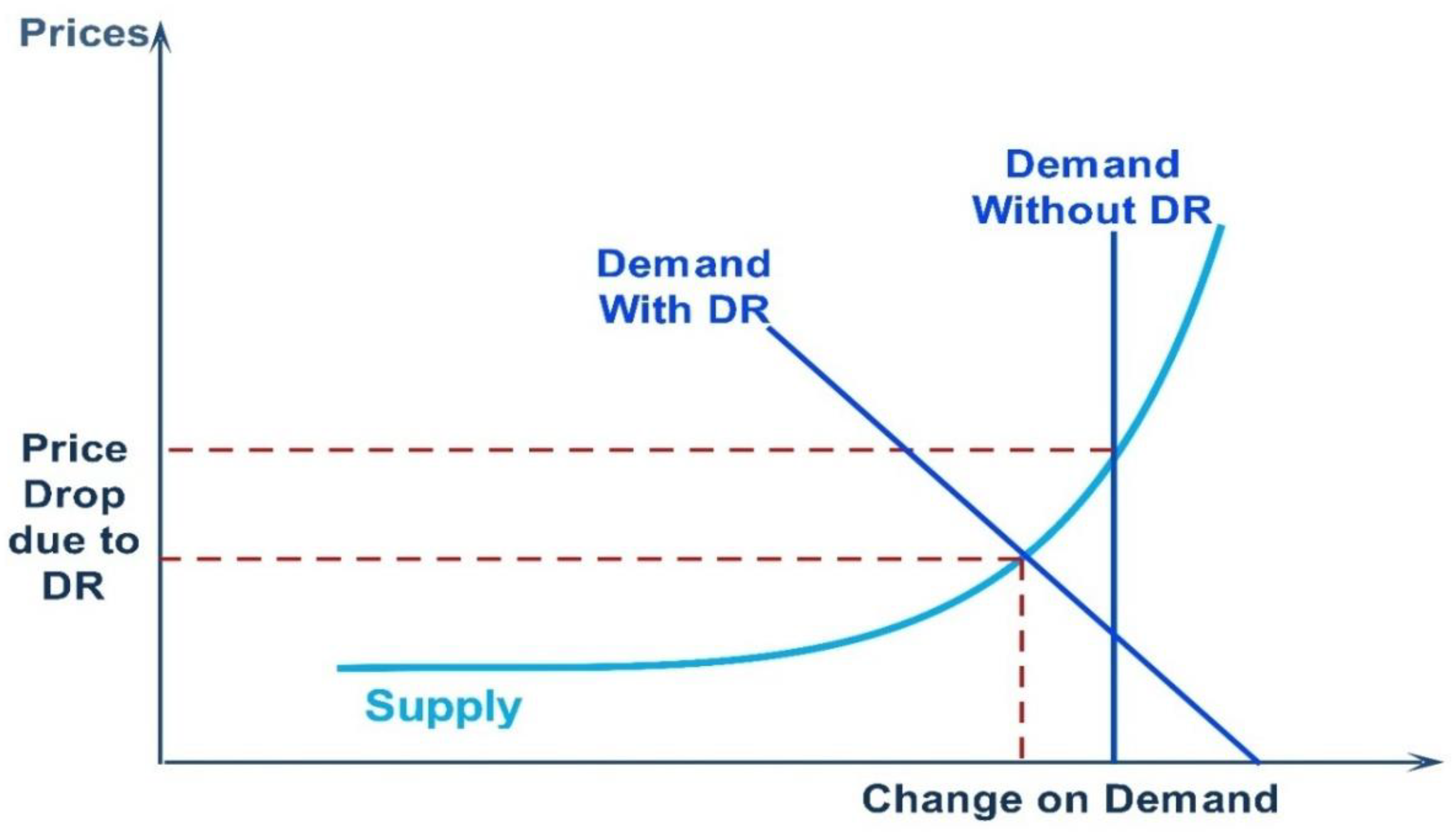
For an efficient operation, the supply and demand in the electricity system must be perfectly synchronised in real time. However, this is not always the case because of the complexity of the system and the fact that supply and demand levels frequently change because of a variety of factors, such as the failure of a generation unit, a transmission or distribution line, or a sudden change in load. DR is one of the least expensive resources available for the system’s best operation because the infrastructure of the power system is substantially capital accelerated [
3]. The decrease in price volatility in the wholesale market is another significant market gain. As illustrated in
Figure 1, a slight decrease in demand would cause a significant decrease in the cost of production and the price of power in real time.
Classifications and Benefits of Demand Response Program
Various DR applications are displayed in
Figure 2. Incentive-based programmes (IBP) and price-based programmes (PBP) are the two basic types into which DR programmes can be categorised [
3,
8]. IBP can also be broken down into two categories: traditional and market based. Direct load control (DLC) and interruptible or curtailable services (I/Cs) are examples of traditional applications. Emergency disaster relief initiatives (EDRP), demand bidding (DB), capacity market programmes (CMP), and ancillary services market programmes are the four categories for market-based programmes (ASMP).
PBP plans are based on spirited pricing rates, which means that electricity costs do not follow a flat rate pattern but instead vary hourly. Time of use (TOU) pricing, real time pricing (RTP), and the critical peak price (CPP), which is further separated into two categories: extreme day price (EDP), extreme CPP, are the three basic categories in which these rates are categorised (ED-CPP).
Figure 3 displays the advantages of DR. They were classified into four groups: market side, participant side, dependability side, and market fulfilment.
The benefits of DR programmes do not just benefit the members’ wellbeing, some of them are also market focused. For instance, a decrease in the total demand lowers the cost of newly installed generating units. Because they have an impact on all programme participants, reliability assets might be regarded as one type of market-focused help [
9].
The final DR programme category is enhancing electricity market fulfilment [
10]. Using market-based programmes and spirited pricing strategies, consumers can manage the power of the market [
11,
12].
Due to the increasing demand, simple remedies to the issue include the construction of new transmission corridors and the bolstering of current power assets. However, they are pricey, take a while to produce, and may not be achievable because of space limitations. Before new or improved grids are available, renewable power plants, such as wind turbines and solar panels, can be quickly commissioned and made ready for electricity generation. Due to this mismatch, newly constructed renewable plants may experience full or partial curtailments, which may have unfavourable technical and economic effects [
13,
14].
This conundrum can be resolved by utilising one of the numerous options provided by the “smart grid” concept to operate current grids with an enhanced flexibility. The dynamic thermal rating (DTR) technique, which safely establishes the thermal limits of power components based on ambient variables, is the subject of this study. DTR is sometimes referred to as real-time thermal rating (RTTR) or flexible thermal rating because the power rating of this system fluctuates over time and appears flexible (FTR) [
13,
14]. Demand response, the dynamic thermal rating system, and battery energy storage systems (BESS) have all become more significant components of global power grids. Without impairing network dependability, DTR and DR lower the requirements for BESS sizing [
15]. The integration of the wind and demand response for the optimum generation reliability, cost, and carbon emissions is given in [
16]. To lessen the network congestion, operating costs, and wind curtailment, the dynamic thermal rating (DTR) system and the battery storage system (BSS) is used. The improved wind penetration and dependability through network topology optimization based on the dynamic thermal rating and battery storage systems is given in [
17].
This paper has certain benefits:
In this paper, load shifting, and strategic conservation techniques have been employed. The residential and commercial sectors have served as test datasets for various DSM techniques:
Using a unique population-based meta-heuristic optimization technique known as the RUNge Kutta optimizer (RUN), the control of the switching of multiple devices of different classes in each test smart grid has been achieved.
Calculated the decrease in operational costs and peak demand and contrasted the output from the RUNge Kutta optimizer (RUN) with the whale optimization algorithm (WOA), slime mould algorithm (SMA), Sine Cosine Algorithm (SCA), and moth–flame optimization (MFO).
Proved the efficacy of RUN over WOA, SMA, SCA, and MFO.
The other sections of the paper are organised as follows:
Section 2 discusses DR approaches,
Section 3 discusses problem formulation and RUN,
Section 4 provides information on the smart grid, and
Section 5 reports the simulation results. The research’s key findings are finally presented in the form of a conclusion.
2. Techniques in Demand Response
To produce the desired changes in the load contour at the distribution side, DSM modifies the power consumption. DSM focuses [
18] on energy-saving techniques, electricity tariffs, financial incentives, and user- and environmentally friendly government policies to prevent the peak demand. Due to an increase in electricity demand, the system becomes unstable. To prevent these instabilities, demand side management has established a worthy objective that could be used to change the load curve’s configuration by reducing and shifting the total load demand at the distribution side during peak load periods to lower the electricity’s final tariff. Peak clipping, load shifting, valley filling, load growth, strategic conservation, and the flexible load curve are six broad techniques that can be used to alter the load configurations that depict the daily electric demands of residential, commercial, and industrial consumers between peak and off-peak times [
18,
19].
Figure 4 depicts these six demand side management topologies. To reduce the fear of smart grid insecurity, peak clipping and valley filling strategies focused on levelling the peak and valley load levels. Direct load control (DLC) is a technique used in the peak clip approach [
18,
19]. Load shifting, which involves moving loads from peak consumption times to off-peak consumption times, is a load management approach that is successfully used throughout the world [
18,
19]. To achieve load shape optimization, strategic conservation [
18] seeks to directly deploy demand curtailment techniques at client residences. Strategic load expansion [
18,
19] is employed in cases of high demand to optimise the daily response, and it roughly equates to the valley fill strategy. Flexible load shape is primarily related to the dependability of the smart grid [
18,
19].
A singular approach to achieving the best result, given the constraints, is optimization. The objective of the optimization procedures should be to maximise profit and reduce loss or effort. In this research, optimization algorithms have been used to minimise the load and lower operational costs. In the context of meta-heuristic algorithms, a useful literature review is provided in the following methods to comprehend the fundamentals of DSM with applications.
In recent years, meta-heuristic algorithms have gained attention thanks to their special ability to apply derivative-free techniques to problems in the actual world. These algorithms’ structures are very simple to apply to actual problems and are based on ideas about life, phenomena, and particle activity.
The adaptability of these algorithms demonstrates their suitability for the application portion. There have been numerous meta-heuristic optimization approaches reported in the literature to solve DSM problems.
The widely accepted Darwinian theory is the foundation of the genetic algorithm (GA), which is utilised all over the world [
10,
11,
12,
20,
21]. To improve the overall efficiency of the smart grid, authors in [
10] minimised the peak to average ratio (PAR), [
11] developed a DSM system for buildings using the GA, [
12] solved the economic load dispatch problem under demand response, and [
20] and [
21] held the energy consumption scheduling which gave the demand response optimization model for home appliances. Evolutionary algorithms [
22,
23] and biogeography-based optimization algorithms [
24,
25] are other examples of these methods. Evolutionary algorithms are employed for residential energy management in [
23] and evolutionary game theory has been used to investigate the various aspects influencing user demand participation in [
22]. To address energy scheduling issues, biogeography-based optimization has been used to smart homes [
24], smart grids [
25], and to achieve countable cost reductions while reducing the peak load [
26]. When discussing these algorithms, the flow begins with the initial solution set and progresses through runs as various operators are incorporated. Particle swarm optimization was used for hourly grid scheduling [
27], an optimal battery energy storage schedule [
28], the demand response for residential consumers [
29], and an economic load dispatch problem [
30]. The cuckoo search optimization algorithm was used for the optimal scheduling of time-shiftable loads [
31,
32], spider monkey optimization (SMO) was used for DG allocation for demand side management [
33], the bat algorithm was used to optimise the cost in the HEM system [
34], firefly optimization used to construct the efficient DSM system [
35], and in this flow, fruit fly optimization was used for the load balancing of the applications of EHR [
18], and the grasshopper optimization algorithm [
19] was used to design an efficient energy management in office. The gravitational search algorithm was used to solve the unit commitment problem for electric vehicles in [
36] and the optimal scheduling of building users’ electricity consumption in [
37]. A hybrid BBBO was used to address the economic load dispatch (ELD) problem [
38] and the Lyapunov optimization strategy was used to explore power efficiency for residential consumers [
39].
In this paper, many shiftable and programmable devices with new load patterns were used. In the same way, this issue is viewed as an optimization issue and a novel population-based metaheuristic optimization algorithm based on the RUNge Kutta method have been applied to solve this kind of challenging issue. In this research, optimization algorithms have been used to minimise the load and operational costs.
3. Used Demand Response Technique
Strategic conservation and load shifting strategies, an advanced DSM methodology, have been applied in this work to govern a future smart grid. Utilized DSM approaches should aim to always reduce peak demand and energy costs. Future smart grid engineers are always working to create an effective load curve optimization to achieve the DSM programmes’ primary objective.
3.1. DSM Problem Formulation
There are so many optimization techniques in the past literatures which may be used to solve complex DR problem [
36]. DSM techniques always tried to bring the load curve as near to the objective curve as possible and optimization algorithms are trying to overlap both to achieve better results [
37]. The mathematical formulation for strategic conservation and the load shifting technique are given below:
Minimization objective:
where abbreviations are:
t = time period
objective (t) = objectives value at time t.
C Load (t) = exact utilization at given time t.
At any instance for strategic conservation, exact utilization, and
C Load (
t) can be drawn by Equation (2):
where abbreviations are:
On-off status of any devices ranging from= i to N,
Specific class of any device given by= j to D.
Z = summation of devices in a specific class.
At any instance for load shifting, exact utilization and
C Load (
t) is given by Equation (3):
where abbreviations are:
= forecast load at time t.
and = amount of loads and at time t.
3.2. Overview of RUNge Kutta Method
To solve ordinary differential equations, the RUNge Kutta method (RKM) is broadly used [
40,
41]. By employing functions without requiring their high-order derivatives, the RKM can be used to produce a high-precision numerical approach [
42]. The following is a description of the RKMs fundamental formulation.
Consider the following first-order ordinary differential equation for an initial value problem:
To define as the slope (S) of the best straight line fitted to the graph at the point, is the primary concept behind the RKM. Using the slope at point , another point can be obtained by using the best fitted straight line: , where . Similarly, . This process can be repeated m times, which yields an approximate solution in the range of .
The RKM is derived from the Taylor series, which is provided by:
The following approximation equation can be produced by removing the higher-order terms.
The first order RUNge Kutta formula, sometimes known as the Euler formula, can be written as follows:
where
and
The central differencing formula shown below can be used to approximate the first-order derivative (
y′(
x)) [
43]:
Thus, Equation (7) can be rewritten as:
The fourth order RUNge Kutta (RK4) [
44] was employed in this work to construct the suggested optimization approach. The RK4 method’s formula, which is based on the weighted average of four increments (as depicted in
Figure 5) is as follows:
are the four weighted factors and their relative values are as follows:
where
is the first increment and uses
to calculate the slope at the start of the range
. In the second increment,
, the slope at the midpoint is specified using
and
, in the third increment,
, the slope at the midpoint is defined using
and
, and in the fourth increment,
, the slope at the end of the interval is specified using
and
. The next value,
is defined by the current value,
plus the weighted average of the previous four increments, according to RK4.
3.3. Introducing the RUNge Kutta Optimizer (RUN)
Meta-heuristic algorithms (MAs) avoid the contingencies of all local optima and allow algorithms to search for optimal solutions in each search area, in contrast to deterministic algorithms which follow the rituals of a lack of randomness that drag into local optima sinking. Some gradient descent methods perform better than MAs in linear optimization issues in terms of efficiency and convergence rate. When there is no need for gradient information, MAs can successfully produce random solutions to real problems in non-linear problems. Among the actual problems, the main one is the potential for the solution space to grow infinitely and become indefinable, making it difficult to identify the top answer in the available search space. In this case, MAs randomly sample the solution space to find the upcoming best solution while adhering to resource limitations or minimising computational complexity. The finest solutions are generated by MAs using physical principles or biological events. These algorithms are based on concepts of life, phenomena, and behaviour particular to that setting and keep relatively simple structures that are straightforward to apply to actual situations without affecting their structure. Because of their versatility, MAs are clearly effective in the application sector.
MAs have the following notable characteristics:
MAs are algorithms that use natural laws to solve challenging real-world issues. They are inspired by nature.
MAs acquire a stochastic nature when random components are added.
Because the algorithm does not use derivatives, it takes less time.
With the help of many control parameters, MAs are customised to the nature of the issue.
This study develops a new swarm-based model with stochastic elements for optimization. With emphasis on the mathematical core as some sets of active rules at the appropriate time, this model removes the cliche inspiration attachment with itself and the recommended RUN technique. Metaphors are not allowed in population-based models since they simply serve to conceal the true nature of the equations used in the optimizers.
RUN explains the fundamental reasoning behind the RK method as well as the population-based evolution of a group of agents. To calculate the slope and resolve the ordinary differential equations, the RK use a particular formulation (the RK4 method) [
40,
41]. The fundamental concept of RUN is the RK method’s recommended estimated slope. The RUN builds a set of rules for the evolution of a population set in accordance with the logic of the swarm-based optimization algorithm by using the calculated slope as a searching logic to explore the potential area in the search space. The next subsections go into more detail into the RUNs mathematical formulation.
3.3.1. Initialization Step
The logic in this step is to select an initial swarm and let it evolve within the permitted number of iterations. For a population of size N, the N locations are produced at random in RUN. Everyone in the population
is a D-dimensional solution to an optimization problem. Generally, the following concept creates the initial positions at random:
where rand is a random number between [0, 1] and
and
are the lower and upper limits of the problem’s
variable (l = 1, 2,..., D). This rule merely produces a limited number of solutions.
3.3.2. Root of Search Mechanism
Any optimizer’s ability to generate the exploration and exploitation patterns iteratively depends on its iterative cores. In the exploration core, an optimization algorithm explores the promising regions of the feasible space using a collection of random solutions with a high unpredictability rate. The exploitation of core solutions and random behaviours exhibit considerably smaller and more gradual fluctuations than the exploration process [
45]. The RK approach is used in this work to conduct a proper global and local search while searching the decision space using a collection of random solutions.
The proposed RUN’s search mechanism was determined using the RK4 approach. The coefficient
, derived by Equation (8), was defined using the first-order derivative. Therefore,
is defined as:
where
, and
are three randomly selected solutions taken from the population, (
), and
are the worst and best solutions acquired at each iteration. Equation (13) can be changed as follows to improve the exploration search and provide a random behaviour:
Overall, finding promising regions and progressing toward the overall best solution are greatly aided by the best solution
. Therefore, in this study, the best solution
is given more weight during the optimization process by using a random parameter
. To specify
in Equation (13), use the formulas:
where
is a parameter and
are the position increment. The step size,
, is established by the difference between
and
. During optimization, parameter
, a scaling factor dictated by the size of the solution space, decreases exponentially. The average of all solutions at each iteration is known as
. The three additional coefficients (i.e.,
) can therefore be expressed as follows:
In this study,
are determined by the following:
Therefore, the leading search mechanism in RUN can be defined as:
3.3.3. Updating Solutions
The RUN algorithm begins the optimization process with a set of random solutions. The RK approach is used to update the solutions’ locations after each iteration. RUN uses a solution and the search algorithm discovered by the RK technique to do this. In this study, the following plan is put into practise to build the position at the subsequent iteration while providing the global (exploration) and local (exploitation) search:
In which, .
Equation (20) is recast as follows to carry out the local search around the solutions
,
and examine the promising regions in the search space:
where
r is an integer that might either be 1 or less than 1. This parameter alters the direction of the search and broadens it. The value of
g is a chance number between [0, 2].
3.3.4. Enhanced Solution Quality
The enhanced solution quality (ESQ) is used in the RUN algorithm to improve the quality of the solutions and avoid local optima in each iteration. The RUN algorithm makes sure that each solution advances toward a higher position by employing the ESQ. In the suggested ESQ, the best position (
) and the average of three random answers (
) are merged to produce a new solution (
). The solution (
) is produced using the ESQ by executing the following scheme:
In which
where
is a random number between [0, 1]. The random number c in this investigation is equal to 5 *rand. The random number w gets smaller as the number of iterations rises. r is an integer that can only be 1, 0, or 1. The best solution explored so far is
. The calculated solution (
) might not be more fit than the existing solution (i.e.,
>
). Another new solution (
) is developed to have a second opportunity at producing a successful solution, and it is defined as follows:
where
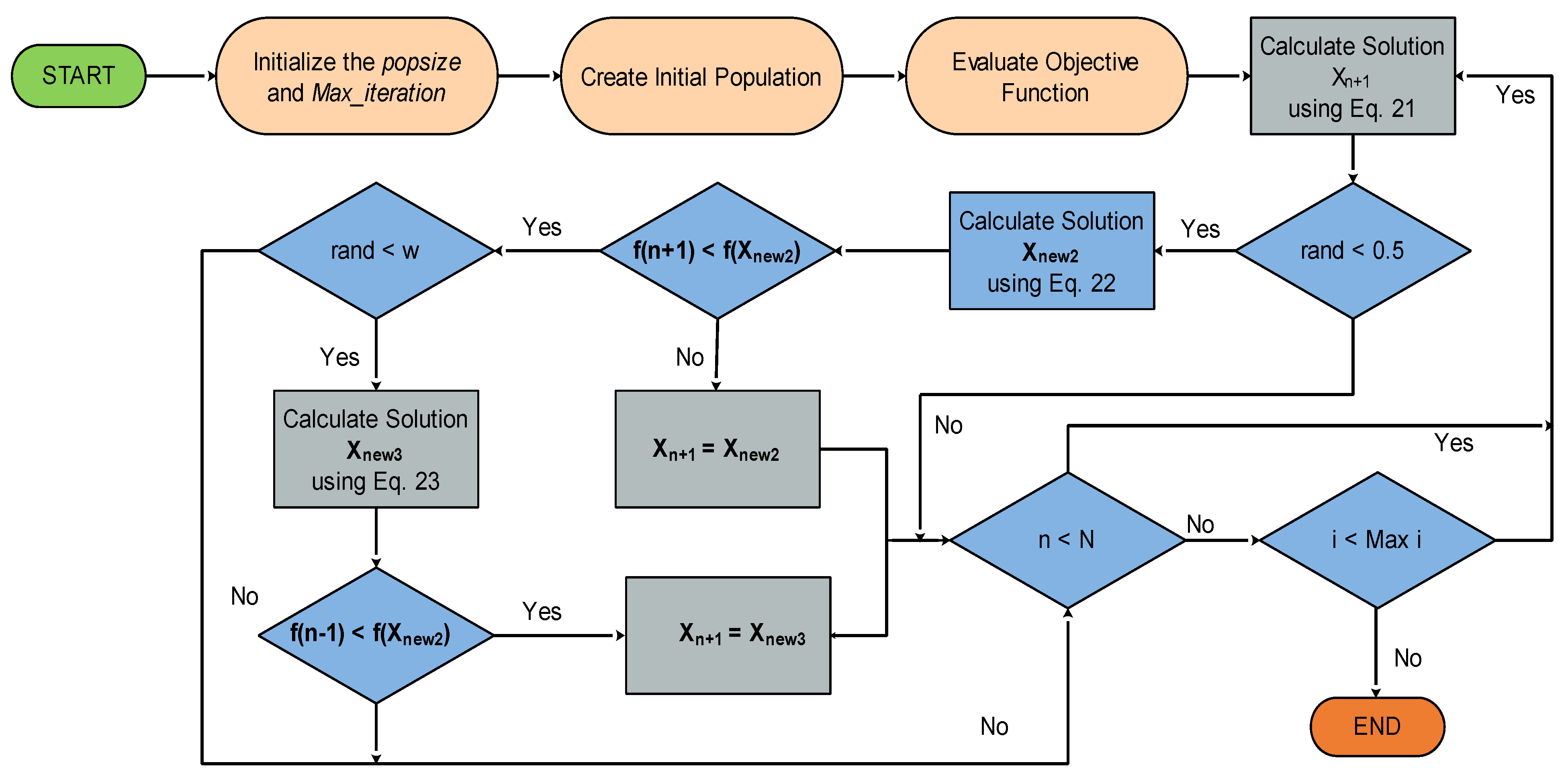
v is a random number with a value of 2*rand. The pseudo-code of the standard RUN is presented in Algorithm 1 and in
Figure 6.
| Algorithm 1. The pseudo-code of RUN [46] |
| Stage 1. Initialization |
| Initialize a and b |
| (n = 1,2, …, N) |
| Determine each population member’s objective function. |
|
| Stage 2. RUN operators |
|
|
|
| Updating solutions |
| using Equation (18) |
| End for |
| Enhance the solution quality |
| |
| using Equation (19) |
|
|
| using Equation (20) |
| End |
| End |
| End |
|
| End for |
|
|
| End |
| Stage 3. Return |
The following qualities theoretically show that the RUN is adept at resolving a range of challenging optimization problems:
The randomised adaption feature of the scale factor (SF) helps RUN further enhance the exploration and exploitation phases. This setting guarantees a seamless changeover from exploration to exploitation.
In the initial iterations, RUNs propensity for exploration can be encouraged by using the average position of solutions.
To improve both exploration and exploitation capabilities, RUN uses a search mechanism based on the RK approach.
The RUN algorithm’s improved solution quality (ESQ) feature makes use of the best solution found so far to increase the solution quality and accelerate convergence.
If the new solution in the RUN algorithm does not place the current solution in a better position, it may be able to identify a new position within the search space to place the current solution in a better position. This method can raise the standard of the solutions and raise the convergence rate.
To highlight the significance of the best solution and progress toward the global best solution, which may successfully balance the exploration and exploitation processes, the search mechanism and ESQ use two randomised variables.
5. Results and Discussion
The utilized DSM technique has enough capability to replicate the load curve with the objective curve, as shown by data tables and figures. The RUN did a great job at handling the minimization problem.
To validate the proposed technique, two test boats have been used.
5.1. Test Boat 1: Strategic Conservation
Appliances that are effective and smart are utilized to decrease load demand in order to maintain the appropriate load shape. Due to the need for a constant supply of electricity in the industrial sector, this technique of demand response is only relevant to residential and commercial consumers.
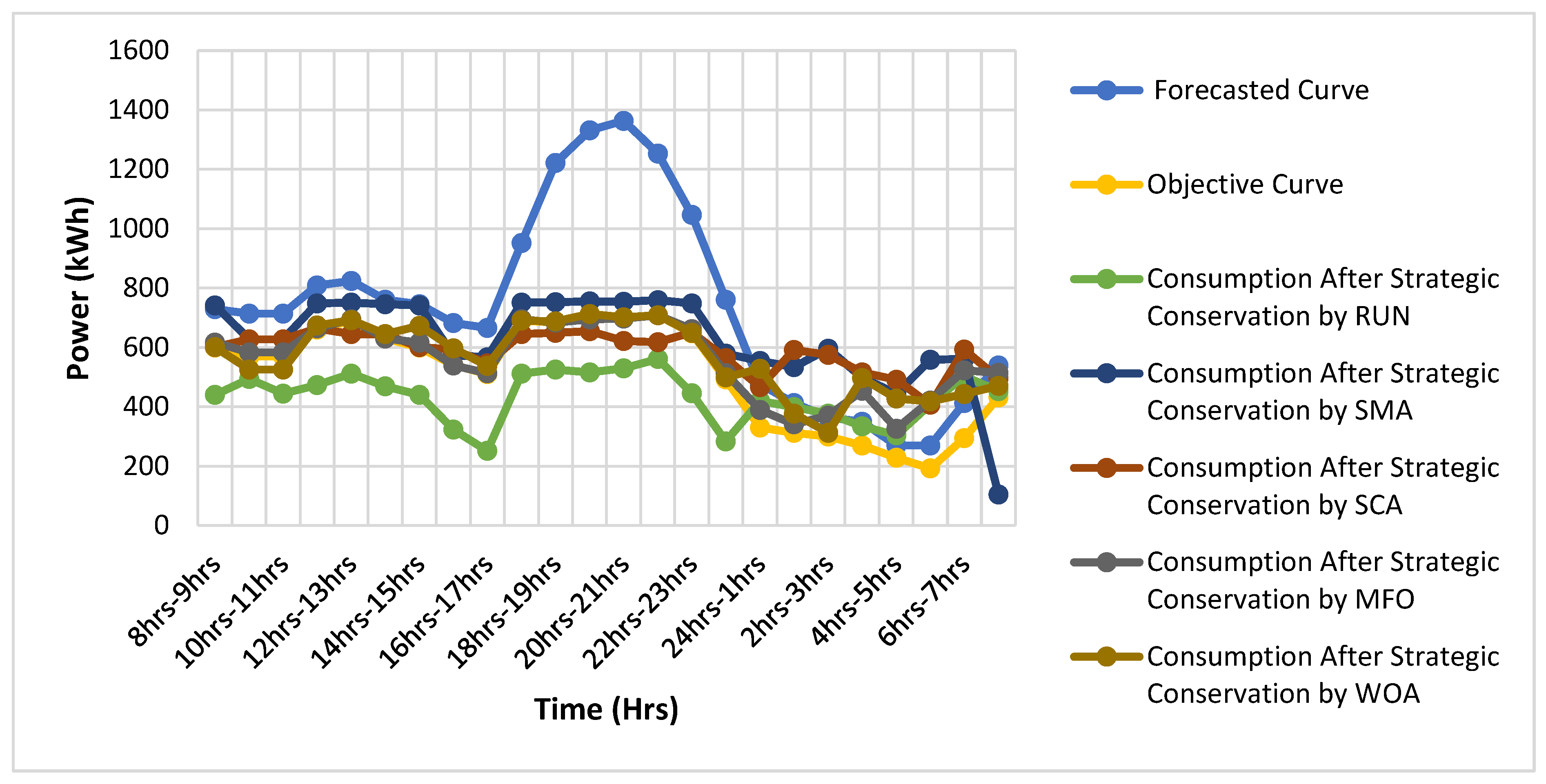
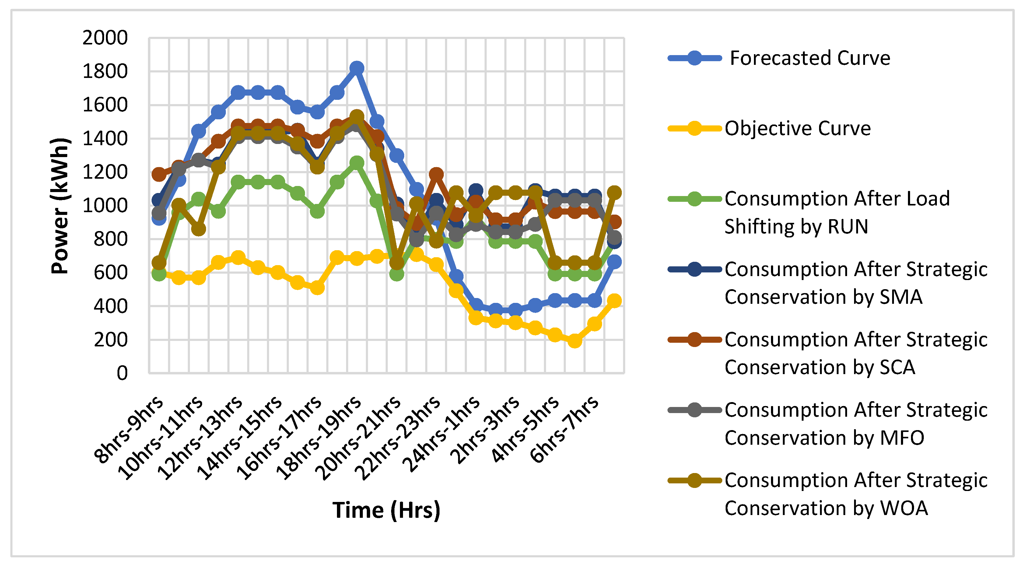
Figure 7 depicted the simulation curves of the residential area from the strategic conservation technique. Table IV shows the comparison of operational cost reduction and peak demand reduction in both areas. For the residential area, curtailment in the cost of the operation using the SMA, SCA, MFO, and WOA is given by 14.73%, 21.79%, 23.77%, and 22.78%, respectively. Here, the RUN proved its efficacy over the SMA, SCA, MFO, and WOA by giving a 42.77% curtailment in the operational cost.
For the commercial area, the curtailment in operational cost using the SMA, SCA, MFO, and WOA is given by 13.94%, 10.47%, 15.35%, and 15.20%, respectively. Here, the RUN again proved its efficacy over the SMA, SCA, MFO, and WOA by giving a 28.90% curtailment in the operational cost. When several devices have been used then proposed, the DSM technique gives the better results.
Figure 8 depicted the simulation curves of the commercial area acquired from the strategic conservation technique.
Table 4 shows the comparison of the operational cost reduction and peak demand reduction in both areas. Several benefits provided when the effective path is selected for the DSM. The reduction in peak demand is the one of the examples of it. For the residential area, the peak reduction using the SMA, SCA, MFO, and WOA is given by 44.67%, 54.42%, 48.87%, and 48.53%, respectively. Here, the RUN proved its efficacy over the SMA, SCA, MFO, and WOA by giving 61.16% in peak reduction.
For the commercial area, the peak reduction using the SMA, SCA, MFO, and WOA is given by 15.85%, 15.85%, 21.71%, and 15.92%, respectively. Here, the RUN again proved its efficacy by giving a 28.87% peak reduction. The peak reduction results in an increase in grid stability and lowers the utility cost.
Figure 9 and
Figure 10 show the reduction in operational cost and peak demand, respectively, for strategic conservation.
5.2. Test Boat 2: Load Shifting:
The load shifting technique is used frequently to shift the load from the peak time to the off-peak time.
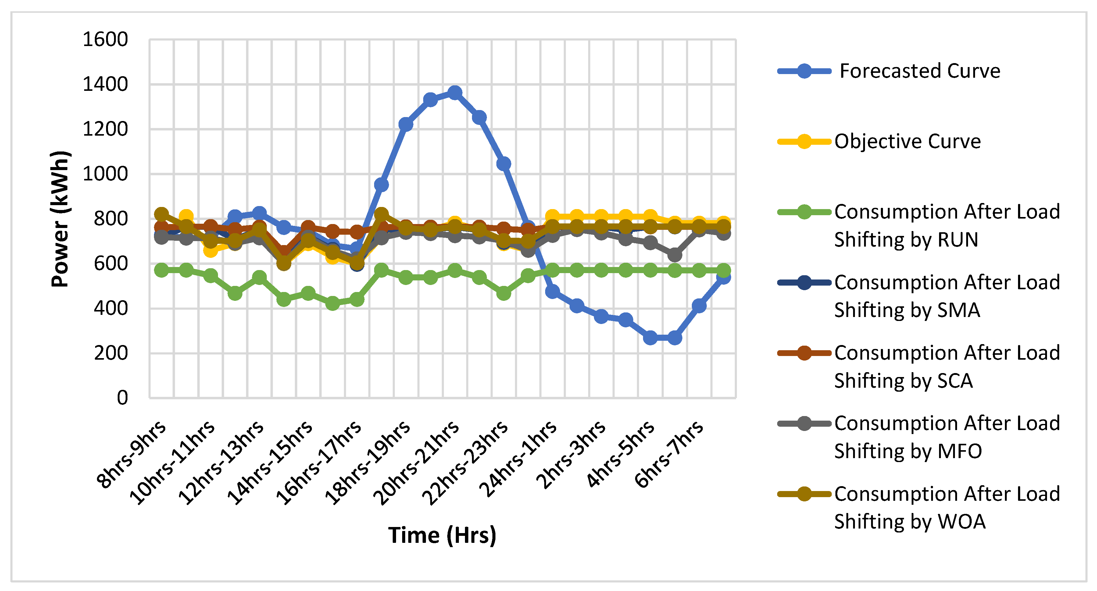
Figure 11 shows the results for residential consumers by using load shifting.
Table 5 encountered the reductions in the operational cost for residential consumers by using the SMA, SCA, MFO, and WOA which is given by 6.26%, 2.36%, 9.40%, and 6.05%, respectively. The RUN proved its iron among other optimization algorithms by giving a reduction in cost by 8.41%. For commercial consumers, a reduction in operational cost by using the SMA, SCA, MFO, and WOA is given by 0.72%, −2.72%, 4.43%, and 6.76%, respectively. The RUN proved its iron over the SMA, SCA, MFO, and WOA by giving a reduction in cost by 16.45%.
Figure 12 reported the simulation results for the commercial area by load shifting. For residential and commercial areas, the peak demand is given by
Table 5. For the residential area, the used DSM technique lowered the peak load by using the SMA, SCA, MFO, and WOA which is given by 44.02%, 43.89%, 46.79%, and 43.89%, respectively. The RUN again gives better results by a 58.26% reduction. For the commercial area, the used DSM technique lowered the peak load by using the SMA, SCA, MFO, and WOA which is given by 15.85%, 15.85%, 18.53%, and 15.92%, respectively. The RUN again gives better results by a 30.97% reduction.
Figure 13 and
Figure 14 show the peak reduction and operational cost, respectively, for load shifting.

 ,
, 


