Article

Some Probabilistic Generalizations of the Cheney–Sharma and Bernstein Approximation Operators

1
Institute of Actuarial Science and Data Analytics, UCSI University, Kuala Lumpur 56000, Malaysia
2
Institute of Mathematical Sciences, Faculty of Science, University of Malaya, Kuala Lumpur 50603, Malaysia
3
Department of Mathematical and Actuarial Sciences, Lee Kong Chian Faculty of Engineering and Science, Universiti Tunku Abdul Rahman, Kajang 43000, Malaysia
4
Department of Mathematics and Statistics, University of Victoria, Victoria, BC V8W 3R4, Canada
5
Department of Medical Research, China Medical University Hospital, China Medical University, Taichung 40402, Taiwan
6
Department of Mathematics and Informatics, Azerbaijan University, 71 Jeyhun Hajibeyli Street, Baku AZ1007, Azerbaijan
7
Section of Mathematics, International Telematic University Uninettuno, I-00186 Rome, Italy
*
Author to whom correspondence should be addressed.
Axioms 2022, 11(10), 537; https://doi.org/10.3390/axioms11100537
Submission received: 22 August 2022 / Revised: 29 September 2022 / Accepted: 29 September 2022 / Published: 8 October 2022

Abstract

:
The objective of this paper is to give some probabilistic derivations of the Cheney, Sharma, and Bernstein approximation operators. Motivated by these probabilistic derivations, generalizations of the Cheney, Sharma, and Bernstein operators are defined. The convergence property of the Bernstein generalization is established. It is also shown that the Cheney–Sharma operator is the Szász–Mirakyan operator averaged by a certain probability distribution.

1. Introduction

Polynomial operators for the approximation of a function have been researched extensively due to the important Weierstrass Approximation Theorem. This theorem states that every continuous function defined on a closed interval can be approximated by a polynomial function. For the approximation of functions, linear positive operators are used because they are computationally simpler. A fundamental operator is the Bernstein operator, defined as follows.
The Bernstein operator of order n, defined on C[0,1], is given by
B n ( f ; x ) = k = 0 n f ( k n ) b n , k ( x ) ,
where f is any real function defined on [ 0 , 1 ] , and b n , k ( x ) is the binomial probability mass function (pmf).
b n , k ( x ) = ( n k ) x k ( 1 x ) n k ,                 k = 0 , 1 , 2 , . , n .
The quantity b n , k ( x ) is also known as the Bernstein basis function.
By starting with the identity (see [1,2])
( 1 x ) α + 1 e ( t x 1 x ) k = 0 L k ( α ) ( t ) x k = 1 ,                     α > 1 ,
Cheney and Sharma [3] defined the operator P n by
  P n ( f ; x ) = ( 1 x ) n + 1 e ( t x 1 x ) k = 0 f ( k k + n ) L k ( n ) ( t ) x k ,
where t 0 ,     0 x 1 and n > 1 , and L k ( n ) ( t ) is the Laguerre polynomial of degree k. The operator P n of Cheney and Sharma corresponds to the pmf
p n , k ( x ; t ) = ( 1 x ) n + 1 e ( t x 1 x ) L k ( n ) ( t ) x k ,                   k = 0 , 1 , 2 ,     ,
which is nonnegative since t 0 and normalized by virtue of (3). When t = 0, Equation (5) reduces to the negative binomial pmf
m α , k ( x ) = ( α + k 1 k ) ( 1 x ) α x k ,                 α = n + 1 > 0 ,     k = 0 , 1 , 2 ,     ,
Then, (4) becomes the Meyer–Konig–Zeller operator:
M n ( f ; x ) = ( 1 x ) n + 1 k = 0 f ( k k + n ) ( n + k k ) x k .
The probabilistic approach to studying approximation operators, in particular, the Cheney–Sharma operator, has been considered, among others, by [4,5]. Cismasiu [6] considered a probabilistic representation of the Szász-Inverse Beta operators. The generalization and construction of approximation operators are still of continuing interest. The main reason for this is that the modified or generalized operators give an improved approximation compared to the original operator. The classic Bernstein operator has been modified and studied by many researchers; see [7,8,9,10]. Some examples of exotic operators are the parametric generalization of Schurer–Kantorovich operators and their bivariate form [11], Baskakov–Schurer–Szász–Stancu operators [12], and Szász–Mirakjan Beta-type operators [13]. In this paper, the probabilistic approach is employed to obtain generalizations of Bernstein and other approximation operators. The motivation for considering this approach is that it provides a systematic method to construct and generalize approximation operators, and the probabilistic setting ensures the positivity of the operators.
In Section 2, we give a probabilistic representation and derivation of the Cheney–Sharma operator. By applying this probabilistic representation to the Bernstein operator (1), we define in Section 3 a generalization of the Bernstein operator (1). The convergence property of this generalization is examined. Further generalizations are also given. Section 4 presents another probabilistic representation of the Cheney–Sharma operator. The Cheney–Sharma operator could also be obtained by averaging the Szász–Mirakyan operator, and this is given in Section 5. Graphical analysis for the generalization of the Bernstein operator is given in Section 6. Section 7 concludes with some remarks.

2. A Probabilistic Representation and Derivation of the Cheney–Sharma Operator

Let N = { N ( λ ) ; λ 0 } be a Poisson process, where N ( λ ) has the pmf given by
p i ( λ ) = e λ λ i i ! ,     λ > 0 ,     i = 0 , 1 , 2 , .  
Let M = { M ( x ; β + i ) ; β 0 ,   0 < x < 1 } be a negative binomial process, with pmf (6) written as a pmf conditional on i:
m β , k ( x | i ) = ( β + i + k 1 k ) ( 1 x ) β + i x k .  
Consider the process P ( x ; β ) = { M ( x ; β + N ( λ ) ) ; λ 0 } , where i varies as a random variable N ( λ ) .This process has pmf given by (5). To see this, consider the unconditional pmf:
m β , k ( x , λ ) = i = 0 m β , k ( x | i ) e λ λ i i ! = e λ ( 1 x ) β x k Γ ( β + k ) k !   Γ ( β ) [ Γ ( β ) Γ ( β + k ) i = 0 Γ ( k + β + i ) Γ ( i + 1 )   Γ ( β + i ) ( λ ( 1 x ) ) i ] = e λ ( 1 x ) β x k   ( β ) k k !   F 1 1   [ β + k ;     β ;     λ ( 1 x ) ] = e λ x ( 1 x ) β x k L k ( β 1 ) ( λ ( 1 x ) )      
where ( β ) k = Γ ( β + k ) Γ ( β ) . Equation (8) is seen as the pmf corresponding to the Cheney–Sharma operator given by (5) with   t = λ ( 1 x ) . To arrive at Equation (8), we have made use of Kummer’s transformation:
F 1 1   [ α ; β ; y ] = e y F 1 1   [ β α ;   β ; y ] .  
and the hypergeometric definition of the generalized Laguerre polynomials:
L n ( α ) ( y ) = ( α + 1 ) n n !   F 1 1   [ n ;   α + 1 ; y ] .  
By applying the above stochastic formulation to the Meyer–Konig–Zeller operator (7), the Cheney–Sharma operator is obtained.
Remark 1.
It is obvious that various generalizations of (6) (and (5)) could be obtained by different choices of the random variable for i. This will then lead to more generalized definitions of the Meyer–Konig–Zeller operator.

3. A Generalization of the Bernstein Operator

Motivated by the probabilistic representation of the Cheney–Sharma operator, we consider a generalization of the Bernstein operator. Let B = { B ( x ; n ) ; n > 0 ,   0 < x < 1 } be a binomial process with pmf (2). As in Section 2, let B = { B ( x ; n + i ) ; n > 0 ,   0 < x < 1 } be a binomial process with pmf:
b n , k ( x | i ) = ( n + i k ) x k ( 1 x ) n + i k ,                     k = 0 , 1 , 2 , , n .  
Let i vary as a Poisson random variable N ( λ ) . By using (10), we obtain the pmf as follows:
q N , k ( x , λ ) = i = 0 b n , k ( x | i ) e λ λ i i ! = ( 1 x ) N k e λ x L k ( N k ) ( λ ( 1 x ) ) x k ,     k = 0 , 1 , 2 , ,
where 0 < x < 1 ,     λ > 0 . We note that, for λ = 0 , (11) reduces to (2), since
L k ( α ) ( 0 ) = ( k + α k ) .  
Rewriting (11) as follows:
q n , k ( y , λ ) = ( 1 y γ ) n k e λ y / γ   L k ( n k ) ( λ ( 1 y γ ) ) ( y γ ) k ,
where y = γ x and γ = 1 + λ n , we define the operator given by
Q n , λ ( f ; y ) = k = 0 f ( k n ) q n , k ( y , λ ) ,
which generalizes the Bernstein operator (1). Operator (13) will be known as the generalized Bernstein operator.
The following theorem considers the convergence property of the operator Q n , λ .
Theorem 1.
If f ϵ C [ 0 , ) and λ n 0 as n , then the sequence of operators { Q n , λ ( f ; y ) } converges uniformly to f(y) on [a, b] where 0 a < b < .
Proof. 
Since Q n , λ is a positive linear operator, we need only to show, using a result of [14] (p. 14), that convergence occurs if f is a quadratic function. We have
k = 0 q n , k ( y , λ ) = 1 ,
k = 0 k q n , k ( y , λ ) = n y ,
k = 0 k 2 q n , k ( y , λ ) = n y γ ( 1 y γ ) + λ y γ + n 2 y 2 .
To derive (14), (15), and (16), consider the moment-generating function of (11):
M ( z ) = k = 0 e z k q n , k ( x , λ ) = [ ( 1 x ) + x e z ] n e ( λ [ ( 1 x ) + x e z 1 ] ) ,
which is easily derived with the help of the following formula ([2] (pp. 84); [15] (p. 189)):
k = 0 L k ( α k ) ( x ) z k = e x z ( 1 + z ) α .
Then, Equations (14)–(16) correspond to M ( 0 ) ,   M ( 0 ) , and M ( 0 ) , respectively, with x = y γ   . The uniform convergence of Q n , λ ( f ; y ) follows from the following observations:
Q n , λ ( 1 ; y ) = 1 , Q n , λ ( s ; y ) = y , Q n , λ ( s 2 ; y ) = y 2 + λ y γ n 2 + 1 n   y γ   ( 1 y γ ) y 2 .
Next, we consider the order of approximation of a function f by the operator Q n , λ .
Theorem 2.
If f ϵ C [ 0 , a ] , then
| f ( y ) Q n , λ ( f ; y ) | 3 2 ω ( 1 + λ n n ) ,
where ω ( δ ) = ω ( f ; δ ) = s u p | f ( x 2 ) f ( x 1 ) | ;   x 2 , x 1 ϵ [ 0 , a ] , such that
| x 2 x 1 | < δ , δ > 0 .
Proof. 
Following [5] (pp. 1185–1186), we obtain
| f ( y ) Q n , λ ( f ; y ) | ( 1 + 1 δ k = 0 q n , k ( y , λ ) | y k n | ) ω ( δ ) { 1 + 1 δ [ k = 0 q n , k ( y , λ ) ( y k n ) 2 ] 1 2 } ω ( δ ) .
By using (14), (15), and (16), we obtain
k = 0 ( y k n ) 2 q n , k ( y , λ ) = y 2 Q n , λ ( 1 ; y ) 2 y Q n , λ ( s ; y ) + Q n , λ ( s 2 ; y ) = 1 n 2 { n y γ ( 1 y γ ) + λ y γ } γ 2 4 n .
The inequalities (17) and (18) lead to
| f ( y ) Q n , λ ( f ; y ) | { 1 + 1 δ γ 2 n } ω ( δ ) ,
and the result follows from choosing δ = γ n .   We can observe that, for λ = 0 , the inequality reduces to the inequality of [16] for the Bernstein operator (1):
| f ( x ) B n ( f ; x ) | 3 2 ω ( 1 n ) .
We next consider immediate generalizations of operators (4) and (13), which are achieved by taking α = β + r I and n = N + r I in (8) and (11), respectively, where r is an integer constant. The generalization of (8) is given by
m β , k * ( x , λ , r ) = ( β ) k k !     e λ x k ( 1 x ) β F r r   [ Δ ( r , β + k ) ;   Δ ( r ,   β ) ; λ ( 1 x ) r ] ,
where Δ ( r ,   α ) stands for the set of r parameters:
    α r   ,   ( α + 1 ) r ,   ,   ( α + r 1 ) r  
and F r r   is the generalized hypergeometric function (see [17]). The following formulas have been employed in evaluating (19) (see [17]):
( a + n ) N = ( a ) N ( a + N ) n ( a ) n , ( a ) k n = ( a k ) n ( ( a + 1 ) k ) n ( ( a + 2 ) k ) n ( ( a + k 1 ) k ) n ( k ) k n
The generalization of (11) is given by
q N , k * ( x , λ , r ) = ( N k ) x k ( 1 x ) N k e λ F r r   [ Δ ( r , N + 1 ) ; Δ ( r , N + 1 k ) ; λ ( 1 x ) r ] .
Let y = x ( 1 + λ r n ) in (20) and define q n , k * ( y , λ , r ) as in (12). The generalized operators of (4) and (13) are given, respectively, by
P n * ( f ; x ) = k = 0 f ( k k + n ) m β , k * ( x , λ , r ) , Q n , λ * ( f ; y ) = k = 0 f ( k n ) q n , k * ( y , λ , r ) .

4. Another Probabilistic Representation of the Cheney–Sharma Operator

Let the logarithmic-series (log-series) distribution [18] with a parameter θ be defined by
p ( k ) = α θ k k ,     k = 1 , 2 , 3 , ,
where 0 < θ < 1   and   α = [ l n ( 1 θ ) ] 1 . We wish to consider a weighted version of the log-series distribution.
Definition. 
Let X be a random variable with pmf p ( k ) . Suppose that the probability of ascertaining the event { X = k } has a weighting factor w ( k ) . Then, the weighted distribution [19] with the weight w ( x ) has pmf given by
P ( k ) = P ( X = k ) = w ( k ) p ( k ) w ( x ) p ( x ) .
Let w ( x ) = k + τ ,   τ 0 be the weight for log-series distribution. The weighted log-series distribution has pmf given by
k   ( τ , θ ) = ( k + τ ) ( 1 θ ) θ k k ( θ τ ( 1 θ ) l n ( 1 θ ) ) .
Suppose that L n ( τ ; θ ) = X 1 + X 2 + X 3 + .     .     . + X n , where X i ,     i = 1 ,   2 ,   .     .     .     . ,   n have pmf (21), that is, L n ( τ ; θ ) is the convolution of n weighted log-series random variables.
Theorem 3.
Let L = { L n ( τ ; θ ) } be the n-convolution weighted log-series process with pmf k   ( τ , θ ; n ) conditional on n as a Poisson random variable N ( λ ) . Then, the unconditional distribution has pmf given by
β , k ( x , λ ) = e λ x ( 1 x ) β x k L k ( β 1 ) ( λ ( 1 x ) )
where x = θ ,   τ = β / λ ( 1 θ ) .
Proof. 
It is simpler to prove the result by using a probability-generating function (pgf). The pgf of the log-series distribution is given by
g ( t ; θ ) = l n ( 1 θ t ) l n ( 1 θ ) ,     i n   t 1 .
It follows that the pgf of the weighted log-series distribution is given by
g ( t ; θ , τ ) = 1 θ θ τ ( 1 θ ) l n ( 1 θ ) { θ t 1 θ t τ l n ( 1 θ t ) } .
The pgf of the n-convolution is g ( t ; θ , τ ) n . The unconditional pgf with n as a Poisson random variable N ( λ ) is given by
g ( t ; θ , τ , λ ) = n = 0 g ( t ; θ , τ ) n e λ λ n n ! = exp { λ ( g ( t ; θ , τ ) 1 ) } .
Let x = θ ,   τ = β / λ ( 1 θ ) in g ( t ; θ , τ , λ ) . Then,
g ( t ; θ , τ , λ ) = g ( t ; x , β , λ ) = exp { λ ( 1 x 1 x t 1 ) } ( 1 x 1 x t ) β .
By applying the generating function (see [2] (pp. 84) and [15]):
k = 0 L k ( α ) ( x ) z k = e x z / ( 1 z ) ( 1 z ) ( α + 1 ) ,
the pmf (22) is obtained. This is the pmf corresponding to the Cheney–Sharma operator. □

5. Cheney–Sharma Operator as Average of Szász–Mirakyan Operator

Consider the operator given by
R n ( f ; x ) = 0 S n ( f ; u ) g ( u ; x ) d u
where g ( u ; x ) is a probability density function (pdf), and S n ( f ; u ) is the Szász–Mirakyan operator (see [20] (p. 553))
S n ( f ; u ) = e n u k = 0 ( n u ) k k ! f ( k n ) .
By rewriting (23) as follows:
R n ( f ; x ) = k = 0 f ( k n ) { 0 e n u ( n u ) k k ! g ( u ; x ) d u } ,
the integral in braces may be thought of as the counting distribution P k ( t ) of a mixed Poisson process with the mixing distribution g ( u ; x ) :
P k ( t ) = 0 e t u ( t u ) k k ! g ( u ; x ) d u
(see [21] (pp. 35–36)).
Clearly, various generalizations of the Szász–Mirakyan operator could be obtained by appropriate choices of g ( u ; x ) . In particular, if
g ( u ; a ) = ( n a ) n + 2 2 ( u λ ) n 2 e ( λ + n a u )   I n [ 2 λ n a u ] ,     a , λ , n , u > 0
is the pdf of the Bessel function distribution of Laha [22], then R n is the Cheney–Sharma operator (4).
Theorem 4.
If g ( u ; a ) is given by (25), then the operator R n ( f ; a ) is given by
R n ( f ; a ) = k = 0 f ( k n ) e λ 1 + a ( 1 1 + a ) k ( a 1 + a ) n + 1 L k ( n ) ( λ a 1 + a ) .
Proof. 
To prove (26), we note from (24) that we only need to evaluate the following integral:
I = 0 e n u ( n u ) k k ! g ( u ; a ) d u .
We thus obtain
I = 0 e n u ( n u ) k k ! g ( u ; a ) d u = e λ ( a 1 + a ) n + 1 ( 1 1 + a ) k ( n + 1 ) k k ! F 1 1   [ n + 1 + k ; n + 1 ; λ a 1 + a ]
by using the following result [23]:
0 e b 2 y 2 y α 1 I v ( c y ) d y = c ν Γ ( α 2 + ν 2 ) 2 ν + 1 b α + ν Γ ( ν + 1 ) F 1 1   [ α 2 + ν 2 ;   ν + 1 ; c 2 4 b 2 ] ,
where R e ( α 2 + ν 2 ) > 0 , with the following substitution:
y = u ,       b = n ( 1 + a )   ,   α = 2 ( k + n 2 + 1 ) ,   c = 2 λ n a   ,   ν = n .
By applying Kummer’s transformation, Equation (9), and the definition of the generalized Laguerre polynomial (10), we obtain
I = e λ 1 + a ( 1 1 + a ) k ( a 1 + a ) n + 1 L k ( n ) ( λ a 1 + a )
This is the Cheney–Sharma operator P n given by (4), if in Equation (26) we set x = 1 1 + a ,     t = a λ 1 + a , and replace k n by k k + n . □
Remark 2.
(i) The sequence of operators R n ( f ; x ) converges uniformly to f ( x ) on [ a , b ] , where 0 a < b < ,     f C [ 0 , ) when λ n 0 as n . This follows from Korovkin’s theorem and
R n ( 1 ; x ) = 1 , R n ( s ; x ) = x n ( n + 1 + λ ) , R n ( s 2 ; x ) = 1 n 2 [ x ( n + 1 + λ ) + x 2 ( n + 1 + 2 λ ) + x 2 ( n + 1 + λ ) 2 ] .
(ii) Adell et al. [24] gave a probabilistic representation of the Cheney–Sharma operator in terms of a suitable multi-indexed stochastic process. This is to facilitate proof of convergence and to show that it preserves monotonicity and global smoothness.
(iii) The pmf in the Cheney–Sharma operator arises from a photon and neural counting model; see [25] and references therein.

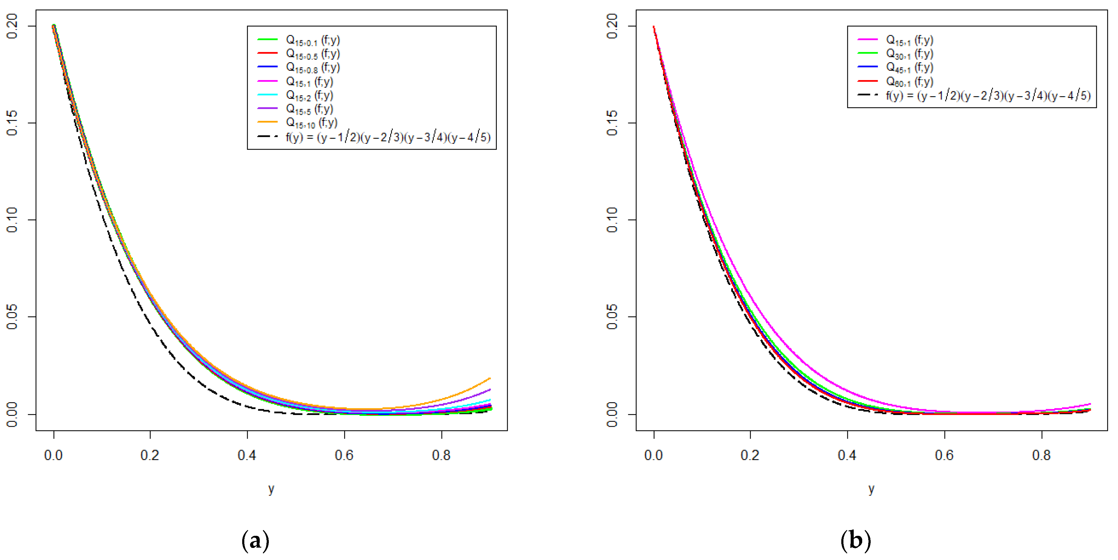
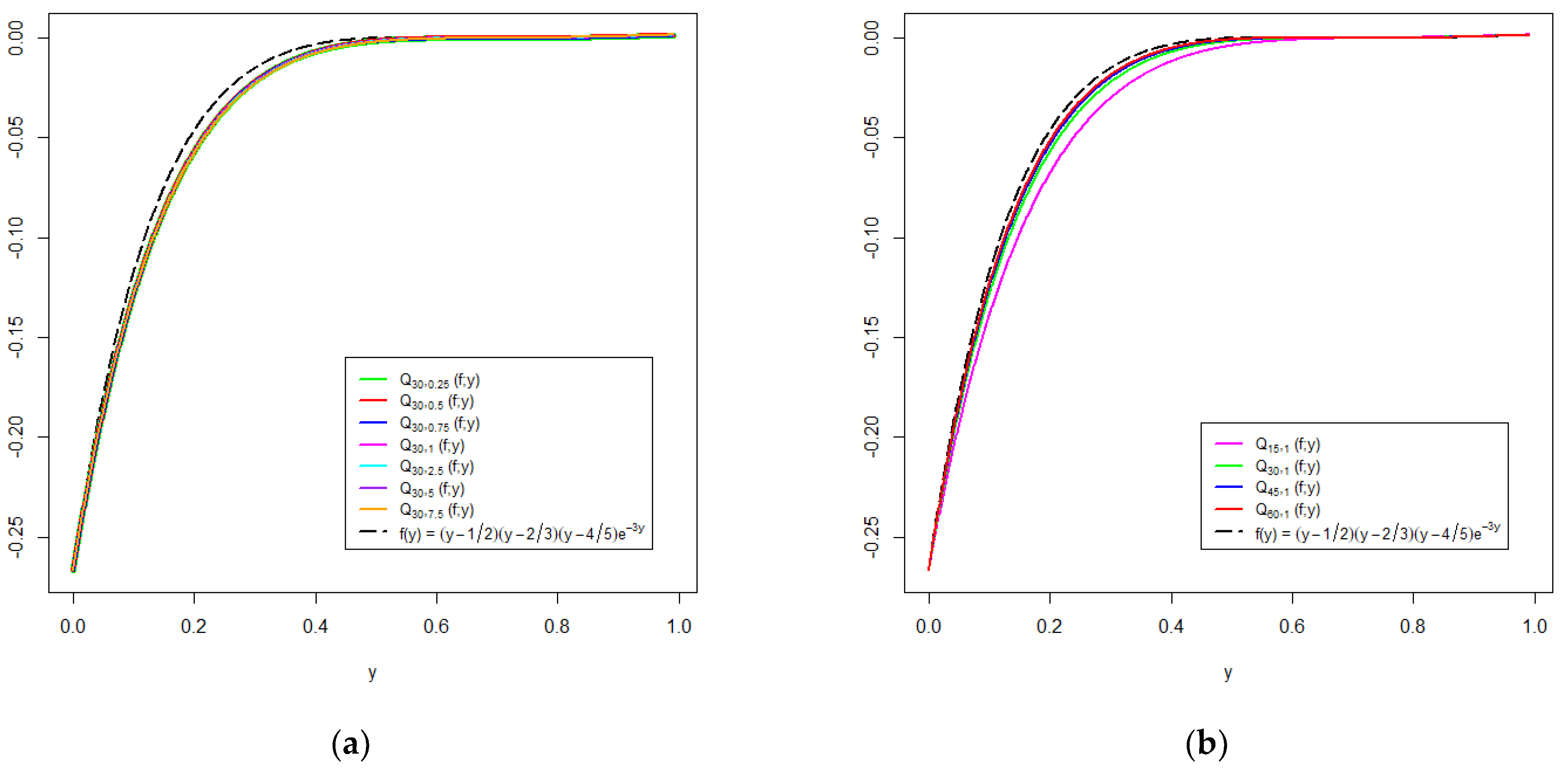
6. Graphical Analysis

The convergence of the generalized Bernstein operator Q n , λ ( f ; y ) given in Equation (13) is demonstrated in this section using the same functions examined in [26]. Taking f ( y ) = ( y 1 2 ) ( y 2 3 ) ( y 3 4 ) ( y 4 5 ) ,   0 y   0.9 , the approximation by Q n , λ ( f ; y ) for the first k = 0 to 125 terms is visualized in Figure 1a for different values of λ , where n = 15 and λ = 0.1 ,   0.5 ,   0.8 ,   1 ,   2 ,   5 ,   10 , and in Figure 1b for different values of n , where λ = 1 and n = 15 ,   30 ,   45 ,   60 .
The maximum error of approximation for Q n , λ ( f ; y ) to the function f ( y ) over the interval [0, 0.9] for different values of λ and n are tabulated in Table 1. It is apparent from these results that the convergence of the operator Q n , λ ( f ; y ) is better when λ / n is smaller.
Next, we examined the approximation to the function f ( y ) = ( y 1 2 ) ( y 2 3 ) ( y 4 5 ) e 3 y over the interval [0, 0.99]. Similarly, the approximation by Q n , λ ( f ; y ) is obtained by taking the sum of the first 125 terms. Figure 2a shows the convergence of Q n , λ ( f ; y ) to the function f ( y ) = ( y 1 2 ) ( y 2 3 ) ( y 4 5 ) e 3 y for different values of λ , where n = 30 and λ = 0.25 ,   0.5 ,   0.75 ,   1 ,   2.5 ,   5 ,   7.5 , while Figure 2b shows the convergence for different values of n , where λ = 1 and n = 15 ,   30 ,   45 ,   60 . Table 2 gives the maximum error of approximation for Q n , λ ( f ; y ) to the function f ( y ) over the interval [0, 0.99] for different values of λ and n . The smallest maximum error of approximation is obtained by taking λ = 0.25 and n = 60 . This combination yields the smallest ratio of λ / n shown in Table 2.

7. Concluding Remarks

In this paper, we have given probabilistic representations of some well-known approximation operators. By extending these probabilistic formulations, generalizations of these approximation operators have been obtained. This probabilistic approach will ensure the positivity of the approximation operators and facilitate the derivation of the moments to prove uniform convergence based on the Korovkin Theorem [14]. This approach also establishes the probabilistic connection between different approximation operators; for instance, the Cheney–Sharma operator as a probabilistic average of the Szász–Mirakyan operator. Further extension of the Cheney–Sharma operator using this averaging process can be constructed by using the results in [27].

Author Contributions

Conceptualization, S.H.O. and C.M.N.; methodology, S.H.O., C.M.N. and H.K.Y.; software, C.M.N.; validation, S.H.O., C.M.N. and H.M.S.; formal analysis, S.H.O., C.M.N., H.K.Y. and H.M.S.; investigation, S.H.O. and C.M.N.; resources, S.H.O. and H.K.Y.; writing—original draft preparation, S.H.O. and C.M.N.; writing—review and editing, S.H.O., C.M.N., H.K.Y. and H.M.S.; visualization, S.H.O. and C.M.N.; supervision, S.H.O.; project administration, S.H.O.; funding acquisition, S.H.O. and H.M.S. All authors have read and agreed to the published version of the manuscript.

Funding

S.H.O. is supported by the Ministry of Higher Education grant FRGS/1/2020/STG06/SYUC/02/1.

Data Availability Statement

Not applicable.

Acknowledgments

The authors wish to thank the reviewers for their insightful comments, which have improved the paper.

Conflicts of Interest

The authors declare no conflict of interest. The funders had no role in the design of the study; in the collection, analyses, or interpretation of data; in the writing of the manuscript; or in the decision to publish the results.

References

  1. Szegö, G. Orthogonal Polynomials; American Mathematical Society Colloquium Publications; American Mathematical Society: Providence, RL, USA, 1959; Volume 23. [Google Scholar]
  2. Srivastava, H.M.; Manocha, H.L. A Treatise on Generating Functions; Halsted Press: Sydney, Australia; Ellis Horwood Limited: Chichester, UK; John Wiley and Sons: New York, NY, USA; Chichester, UK; Brisbane, Australia; Toronto, ON, Canada, 1984. [Google Scholar]
  3. Cheney, E.W.; Sharma, A. Bernstein power series. Canad. J. Math. 1964, 16, 241–252. [Google Scholar] [CrossRef]
  4. Khan, R.A. Some probabilistic methods in the theory of approximation operators. Acta Math. Hung. 1980, 35, 193–203. [Google Scholar] [CrossRef]
  5. Stancu, D.D. Approximation of functions by a new class of linear polynomial operators. Rev. Roum. Math. Pures Appl. 1968, 13, 1173–1194. [Google Scholar]
  6. Cismasiu, C.S. On the Szász-Inverse Beta operators. Stud. Univ. Babeş-Bolyai Math. 2011, 56, 305–313. [Google Scholar]
  7. Wang, M.L.; Yu, D.S.; Zhou, P. On the approximation by operators of Bernstein-Stancu type. Appl. Math. Comput. 2014, 246, 79–87. [Google Scholar] [CrossRef]
  8. Acar, T.; Aral, A.; Gupta, V. On approximation properties of a new type Bernstein-Durrmeyer operators. Math. Slovaca 2015, 65, 1107–1122. [Google Scholar] [CrossRef]
  9. Dong, L.X.; Yu, D.S. Pointwise approximation by a Durrmeyer variant of Bernstein-Stancu operators. J. Inequal. Appl. 2017, 28, 2–13. [Google Scholar] [CrossRef] [PubMed] [Green Version]
  10. Kwun, Y.C.; Acu, A.M.; Rafiq, A.; Radu, V.A.; Ali, F.; Kang, S.M. Bernstein-Stancu type operators which preserve polynomials. J. Comput. Anal. Appl. 2017, 23, 758–770. [Google Scholar]
  11. Nasiruzzaman, M.; Srivastava, H.M.; Mohiuddine, S.A. Approximation process based on parametric generalization of Schurer-Kantorovich operators and their bivariate form. Proc. Nat. Acad. Sci. India Sect. A Phys. Sci. 2022, 92, 301–311. [Google Scholar] [CrossRef]
  12. Braha, N.L.; Mansour, T.; Srivastava, H.M. A parametric generalization of the Baskakov-Schurer-Szász-Stancu approximation operators. Symmetry 2021, 13, 980. [Google Scholar] [CrossRef]
  13. Srivastava, H.M.; İçöz, G.; Çekim, B. Approximation properties of an extended family of the Szász–Mirakjan Beta-type operators. Axioms 2019, 8, 111. [Google Scholar] [CrossRef] [Green Version]
  14. Korovkin, P.P. Linear Operators and Approximation Theory; Hindustan Publishing Corporation: Delhi, India, 1960. [Google Scholar]
  15. Erdélyi, A.; Magnus, W.; Oberhettinger, F.; Tricomi, F.G. Higher Transcendental Functions; McGraw-Hill: New York, NY, USA; London, UK; Toronto, ON, Canada, 1953; Volume 2. [Google Scholar]
  16. Popoviciu, T. Sur l’approximation des function convexes d’ordre supeŕieur. Mathematica 1935, 10, 49–54. [Google Scholar]
  17. Slater, L.J. Generalized Hypergeometric Functions; Cambridge University Press: Cambridge, UK, 1966. [Google Scholar]
  18. Fisher, R.A.; Corbet, A.S.; Williams, C.B. The relation between the number of species and the number of individuals in a random sample of an animal population. J. Anim. Ecol. 1943, 12, 42–58. [Google Scholar] [CrossRef]
  19. Rao, C.R. On discrete distributions arising out of methods of ascertainment. In Classical and Contagious Discrete Distributions; Patil, G.P., Ed.; Statistical Publishing Society: Calcutta, India, 1965; pp. 320–332. [Google Scholar]
  20. Pethe, S.P.; Jain, G.C. Approximation of functions by a Bernstein-type operator. Can. Math. Bull. 1972, 15, 551–557. [Google Scholar] [CrossRef]
  21. Haight, F.A. Handbook of the Poisson Distribution; John Wiley: New York, NY, USA, 1967. [Google Scholar]
  22. Laha, R.G. On some properties of the Bessel function distributions. Bull. Calcutta Math. Soc. 1954, 46, 59–72. [Google Scholar]
  23. Sneddon, I.N. Special Functions of Mathematical Physics and Chemistry; Oliver and Boyd: Edinburgh, UK, 1961. [Google Scholar]
  24. Adell, J.A.; de la Cal, J.; Pérez-Palomares, A. On the Cheney and Sharma operator. J. Math. Anal. Appl. 1996, 200, 663–679. [Google Scholar] [CrossRef]
  25. Ong, S.H.; Toh, K.K.; Low, Y.C. The non-central negative binomial distribution: Further properties and applications. Commun. Stat.-Theory Methods 2021, 50, 329–344. [Google Scholar] [CrossRef]
  26. Sofyalıoğlu, M.; Kanat, K.; Çekim, B. Parametric generalization of the Meyer-König-Zeller operators. Chaos Soliton. Fract. 2021, 152, 111417. [Google Scholar] [CrossRef]
  27. Ong, S.H.; Lee, P.A. On a generalized non-central negative binomial distribution. Commun. Stat.-Theory Methods 1986, 15, 1065–1079. [Google Scholar] [CrossRef]
Figure 1. Convergence of Q n , λ ( f ; y ) to f ( y ) = ( y 1 2 ) ( y 2 3 ) ( y 3 4 ) ( y 4 5 ) for: (a) n = 15 and λ = 0.1 ,   0.5 ,   0.8 ,   1 ,   2 ,   5 ,   10 ; (b) λ = 1 and n = 15 ,   30 ,   45 ,   60 .
Axioms 11 00537 g001
Figure 2. Convergence of Q n , λ ( f ; y ) to f ( y ) = ( y 1 2 ) ( y 2 3 ) ( y 4 5 ) e 3 y for: (a) n = 30 and λ = 0.25 ,   0.5 ,   0.75 ,   1 ,   2.5 ,   5 ,   7.5 ; (b) λ = 1 and n = 15 ,   30 ,   45 ,   60 .
Axioms 11 00537 g002
Table 1. Maximum error of approximation by Q n , λ ( f ; y ) for different values of λ and n over the interval [0, 0.9].
n λ
0.10.50.812510
150.013990.014140.014240.014310.014610.015270.01716
300.007110.007150.007180.007200.007290.007530.00781
450.004770.004790.004800.004810.004850.004970.00513
600.003590.003600.003610.003610.003640.003700.00380
Table 2. Maximum error of approximation by Q n , λ ( f ; y ) for different values of λ and n over the interval [0, 0.99].
n λ
0.250.50.7512.557.5
150.000280.000300.000320.000340.000430.000520.00057
300.000160.000160.000170.000180.000220.000270.00031
450.000110.000110.000120.000120.000140.000170.00019
600.000080.000090.000090.000090.000100.000120.00013
Publisher’s Note: MDPI stays neutral with regard to jurisdictional claims in published maps and institutional affiliations.

