Article

Analytic Representation of Maxwell—Boltzmann and Tsallis Thermonuclear Functions with Depleted Tail

1
Department of Mathematics, Kariavattom Campus, University of Kerala, Thiruvananthapuram 695 581, Kerala, India
2
Office for Outer Space Affairs, United Nations, Vienna International Center, A-1400 Vienna, Austria
*
Author to whom correspondence should be addressed.
Axioms 2021, 10(2), 115; https://doi.org/10.3390/axioms10020115
Submission received: 4 May 2021 / Revised: 1 June 2021 / Accepted: 2 June 2021 / Published: 7 June 2021

Abstract

:
The closed forms of the non-resonant thermonuclear function in the Maxwell–Boltzmann and Tsallis case with depleted tail are obtained in generalized special functions. The results are written in terms of H-function of two variables. The importance of the results in this paper lies in the fact that the reaction rate probability integrals in Maxwell-Boltzmann and Tsallis cases are not obtained by the conventional method of approximation or by means of a single variable transform technique but by means of a two variable transform method. The behaviour of the depleted non-resonant thermonuclear functions are examined using graphs. The results in the paper are of much interest to astrophysicists and statisticians in their future work in this area.

1. Introduction

Thermonuclear reactions taking place in Sun-like stars has received considerable interest in the past few years. The reaction rate probability integrals were obtained in closed forms by using generalized specials functions by many authors, see for example [1,2,3,4]. The evaluation of the reaction rates for low-energy non-resonant thermonuclear reactions in the non-degenerate case is performed using the principles of nuclear physics and kinetic theory of gases [5]. A nuclear reaction in which a particle of type i strikes a particle of type j producing a nucleus p and a new particle q is symbolically represented as i + j p + q . If n i and n j are the number densities of particles i and j, respectively, and if the reaction cross section is denoted by σ ( v ) where v is the relative velocity of the particle and f ( v ) is the normalized velocity distribution, then the thermonuclear reaction rate r i j is obtained by averaging the reaction cross section over the normalized distribution function of the relative velocity of the particles given by [3,6,7].
r i j = n i n j 0 v s . σ ( v ) f ( v ) d v = n i n j σ v i j .
The bracketed quantity σ v i j is the probability per unit time that two particles of type i and j confined to a unit volume will react with each other. For a non-relativistic, non-degenerate plasma of nuclei in thermodynamic equilibrium, the particles in the plasma possess a classical Maxwell–Boltzmann velocity distribution given by [7].
f M B D ( v ) d v = μ 2 π k T 3 2 exp μ v 2 2 k T 4 π v 2 d v ,
where μ is the reduced mass of the particles given by μ = m i m j m i + m j , T is the temperature, k is the Boltzmann constant. Writing in terms of the relative kinetic energy E = μ v 2 2 we obtain the Maxwell–Boltzmann energy distribution as [2,8].
f M B D ( E ) d E = 2 π 1 π k T 3 2 exp E k T E d E .
Using (1) and (3) we have,
r i j = n i n j 8 π μ 1 2 1 k T 3 2 0 E σ ( E ) exp E k T d E .
For a non-resonant nuclear reactions between two nuclei of charges z i and z j colliding at low energies below the Coulomb barrier, the reaction cross section has the form [6,8].
σ ( E ) = S ( E ) E exp 2 π μ 2 1 2 z i z j e 2 E 1 2 ,
where e is the quantum of electric charge, is the Plank’s quantum of action and S ( E ) is the cross section factor which is often found to be constant or a slowly varying function of energy over a limited range of energy given by [3,9].
S ( E ) S ( 0 ) + d S ( 0 ) d E E + 1 2 d 2 S ( 0 ) d E 2 E 2 = ν = 0 2 S ( ν ) ( 0 ) ν ! E ν
Substituting (5) and (6) in (4) we obtain
r i j = n i n j 8 π μ 1 2 1 k T 3 2 ν = 0 2 S ( ν ) ( 0 ) ν ! 0 E ν exp E k T 2 π μ 2 1 2 z i z j e 2 E 1 2 d E .
Putting y = E k T and x = 2 π μ 2 k T 1 2 z i z j e 2 we have
r i j = n i n j 8 π μ 1 2 ν = 0 2 1 k T ν + 1 2 S ( ν ) ( 0 ) ν ! 0 y ν e y x y 1 2 d y .
Thus, the reaction rate probability integral in the Maxwell–Boltzmann case is given by
I 1 ( ν , 1 , x , 1 2 ) = 0 y ν e y x y 1 2 d y .
Let us consider a general form of the integral as
I 1 ( γ 1 , z , x , ρ ) = 0 y γ 1 e z y x y ρ d y , γ C , z > 0 , x > 0 , ρ R + .
Physical situations different from the ideal non-resonant Maxwell–Boltzmann case can be obtained by modification of the cross section σ ( E ) for the reacting particles and/or by the modification of their energy distribution. Some of the non standard physical situations are as follows [4,10,11]:

1.1. Non-Resonant Case with High Energy Cut-OFF

If the thermonuclear fusion plasma is not in a thermodynamic equilibrium then there is a cut-off in the high energy tail of the Maxwell–Boltmann distribution function, then the thermonuclear function to be evaluated takes the form
I 2 d ( ν , 1 , x , 1 2 ) = 0 d y ν e y x y 1 2 d y , x > 0 , d < .
The general form of the integral in this case can be taken as
I 2 d ( γ 1 , z , x , ρ ) = 0 d y γ 1 e z y x y ρ d y , γ C , z > 0 , x > 0 , d < .

1.2. Non-Resonant Case with Depleted Tail

If we consider an ad hoc modification of the Mawell–Boltzmann distribution, this looks like a depletion of the tail of the Maxwell–Boltzmann distribution as suggested by Eder and Motz [12], Clayton et al. [13] and Mathai and Haubold [3], which is given by
I 3 ( ν , 1 , 1 , δ , x , 1 2 ) = 0 y ν e y y δ x y 1 2 d y , x > 0 , δ R + .
We will consider here the general integral of the type
I 3 ( γ 1 , t , z , δ , x , ρ ) = 0 y γ 1 e t y z y δ x y ρ d y ,
where γ C , t > 0 , z > 0 , x > 0 , ρ R + , δ R + .

1.3. Non-Resonant Case with Screening

The electron screening effects for the reacting particles can modify the cross section of the reaction. The reaction rate probability integral in this case will take the form
I 4 ( ν , 1 , b , t , 1 2 ) = 0 x ν e y x ( y + t ) 1 2 d y , x > 0 , t > 0
where t is the electron screening parameter. Here, we consider the general integral as
I 4 ( γ 1 , z , x , t , ρ ) = 0 y γ 1 e z y x ( y + t ) ρ d y , γ C , z > 0 , x > 0 , t > 0 , ρ R + .
The evaluation of the integrals I 1 , I 2 d , I 3 and I 4 in the physical and astrophysical literature are by approximating the integrals by means of the method of steepest descent [6,14,15]. The closed forms of the integrals I 1 , I 2 d , I 3 and I 4 in terms of Fox’s H-function and Meijer’s G-function can be seen in a series of papers by Mathai and Haubold, see for example Haubold and Mathai [7], Mathai and Haubold [4,11] etc. To date, in the literature, the integral I 3 , representing the depleted case, is evaluated in closed form after obtaining approximation of certain terms. In the present paper we will consider the integral I 3 in the depleted case in detail and obtain the closed form evaluation of the function by a different method. Furthermore, we extend the integral to a more general case than the Maxwell–Boltzmann case using the pathway model introduced by Mathai in 2005. Hence the importance of the present study is that it provides the exact analytic solution of I 3 and its pathway extension in closed form.
The paper is organized as follows: In the next section, we consider the general form of the non-resonant reaction rate probability integral in the Maxwell–Boltzmann case with depleted tail and obtain the closed form via the H-function in two variables. A more general form of the depleted non-resonant thermonuclear function is obtained by using the pathway model in Section 3. Section 4 is devoted to studying the behaviour of the depleted non-resonant thermonuclear function in the Maxwell–Boltzmann and Tsallis case and comparing the Maxwell–Boltzmann energy distribution with a more general energy distribution. Concluding remarks are included in Section 5.

2. Standard Non-Resonant Thermonuclear Functions with Depleted Tail

In this section, we evaluate the integral I 3 ( γ 1 , t , z , δ , x , ρ ) and give a representation for it in terms of H-function in two variables. For non-negative integers m 1 , m 2 , m 3 , n 1 , n 2 , n 3 , p 1 , p 2 , p 3 , q 1 , q 2 , q 3 such that 0 m 1 q 1 , 0 m 2 q 2 , 0 m 3 q 3 , 0 n 2 p 2 , 0 n 3 p 3 , for a i , b j , c j , d j , e j , f j C and for α j , β j , A j , B j , C j , D j , E j , F j R + = ( 0 , ) , the H-function in two variables is defined via a double Mellin–Barnes type integral in the form
H x y = H p 1 , q 1 : p 2 , q 2 : p 3 , q 3 m 1 , 0 : m 2 , n 2 : m 3 , n 3 x y ( a j , α j , A j ) 1 , p 1 , ( c j , C j ) 1 , p 2 , ( e j , E j ) 1 , p 3 ( b j , β j , B j ) 1 , q 1 , ( d j , D j ) 1 , q 2 , ( f j , F j ) 1 , q 3 = 1 ( 2 π i ) 2 L 1 L 2 h 1 ( s 1 , s 2 ) h 2 ( s 1 ) h 3 ( s 2 ) x s 1 y s 2 d s 1 d s 2
where
h 1 ( s 1 , s 2 ) = j = 1 m 1 Γ ( b j + β j s 1 + B j s 2 ) j = m 1 + 1 q 1 Γ ( 1 b j β j s 1 B j s 2 ) j = 1 p 1 Γ ( a j + α j s 1 + A j s 2 )
h 2 ( s 1 ) = j = 1 m 2 Γ ( d j + D j s 1 ) j = 1 n 2 Γ ( 1 c j C j s 1 ) j = m 2 + 1 q 2 Γ ( 1 d j D j s 1 ) j = n 2 + 1 p 2 Γ ( c j + C j s 1 )
h 3 ( s 2 ) = j = 1 m 3 Γ ( f j + F j s 2 ) j = 1 n 3 Γ ( 1 e j E j s 2 ) j = m 3 + 1 q 3 Γ ( 1 f j F j s 2 ) j = n 3 + 1 p 3 Γ ( e j + E j s 2 )
and x and y are not equal to zero, and an empty product is interpreted as unity. The contour L 1 is in the s 1 -plane which runs from δ 1 i to δ 1 + i , which separates all the poles of Γ ( b j + β j s 1 + B j s 2 ) and Γ ( d j + D j s 1 ) to the left and all the poles of Γ ( 1 c j C j s 1 ) to the right. The contour L 2 is in the s 2 -plane which runs from δ 2 i to δ 2 + i , which separates all the poles of Γ ( b j + β j s 1 + B j s 2 ) and Γ ( f j + F j s 2 ) to the left and all the poles of Γ ( 1 e j E j s 2 ) to the right. The H-function in two variable given in (17) will have meaning even if some of these quantities are zeros. For details about the contours and existence conditions see Srivastava et al. [16], and Mathai and Saxena [17]. The details of the H-function and G-function in one variable can be seen in [18,19,20].
Let the function f ( x 1 , x 2 ) be defined in R + 2 = ( 0 , + ) × ( 0 , + ) . Then, the Mellin transform of a function f ( x 1 , x 2 ) in points ( s 1 , s 2 ) C 2 is defined as
M f ( s 1 , s 2 ) = 0 0 x 1 s 1 1 x 2 s 2 1 f ( x 1 , x 2 ) d x 1 d x 2
with the inverse
f ( x 1 , x 2 ) = 1 ( 2 π i ) 2 δ 1 i δ 1 + i δ 2 i δ 2 + i M f ( s 1 , s 2 ) x 1 s 1 x 2 s 2 d s 1 d s 2 .
The conditions under which the (21) and (22) are valid have been discussed by Fox [21] and Hai and Yakubovich [22]. Now, consider the integral I 3 ( γ 1 , t , z , δ , x , ρ ) given in (14). We evaluate this integral by using the Mellin transform technique for two variables. Using (21) and
f ( t , z ) = I 3 ( γ 1 , t , z , δ , x , ρ ) = 0 y γ 1 e t y z y δ x y ρ d y ,
we have,
M f ( s 1 , s 2 ) = 0 0 t s 1 1 z s 2 1 0 y γ 1 e t y z y δ x y ρ d y d t d z .
Changing the order of integration due to the uniform convergence of the integral, we obtain
M f ( s 1 , s 2 ) = 0 y γ 1 e x y ρ 0 t s 1 1 e t y d t 0 z s 2 1 e z y δ d z d y = Γ ( s 1 ) Γ ( s 2 ) 0 y γ s 1 δ s 2 1 e x y ρ d y , ( s 1 ) > 0 , ( s 2 ) > 0 .
Putting x y ρ = u we obtain,
M f ( s 1 , s 2 ) = x γ s 1 δ s 2 ρ ρ Γ ( s 1 ) Γ ( s 2 ) Γ s 1 + δ s 2 γ ρ , s 1 + δ s 2 γ ρ > 0 .
Taking the inverse Mellin transform using (22) we obtain,
f ( t , z ) = x γ ρ ρ 1 ( 2 π i ) 2 L 1 L 2 Γ ( s 1 ) Γ ( s 2 ) Γ s 1 + δ s 2 γ ρ ( x 1 ρ t ) s 1 ( x δ ρ z ) s 2 d s 1 d s 2 = x γ ρ ρ H 0 , 1 : 0 , 1 : 0 , 1 1 , 0 : 1 , 0 : 1 , 0 x 1 ρ t x δ ρ z γ ρ , 1 ρ , δ ρ , ( 0 , 1 ) , ( 0 , 1 ) .
where H 0 , 1 : 0 , 1 : 0 , 1 1 , 0 : 1 , 0 : 1 , 0 is an H-function in two variables defined as in (17). If 1 ρ is an integer then put 1 ρ = m , m = 1 , 2 , . Then, using the multiplication formula for gamma function defined by [18,19]
Γ ( m z ) = ( 2 π ) 1 m 2 m m z 1 2 Γ ( z ) Γ z + 1 m Γ z + m 1 m ,
where z C , z 0 , 1 , 2 , . . . and m a positive integer, we have (25) as
f ( t , z ) = m ( 2 π ) 1 m m x m γ m m γ × H 0 , m : 0 , 1 : 0 , 1 m , 0 : 1 , 0 : 1 , 0 x m t m m x m δ z m m δ ( γ , 1 , δ ) , ( γ + 1 m , 1 , δ ) , , ( γ + m 1 m , 1 , δ ) , ( 0 , 1 ) , ( 0 , 1 )
For the non-resonant case with depleted tail, we have γ = 1 + ν , ρ = 1 2 , then, by using the duplication formula for gamma functions, we obtain
I 3 ( ν , 1 , 1 , δ , x , 1 2 ) = 2 π x 2 4 ν + 1 × H 0 , 2 : 0 , 1 : 0 , 1 2 , 0 : 1 , 0 : 1 , 0 x 2 4 x 2 δ 4 δ ( ν 1 , 1 , δ ) , ( ν 1 2 , 1 , δ ) , ( 0 , 1 ) , ( 0 , 1 ) .
Thus, using the H-function in two variables, we have obtained the closed form of the depleted non-resonant thermonuclear function. It is first time ever in the literature the two variable Mellin transform technique has been used to obtain the closed form solution of a non-resonant thermonuclear function and the depleted case in particular, which makes the result important. Next, we obtain the extension of these results by using the pathway model of Mathai which helps in generalizing the present results to a more general framework so that a wider class of integrals are covered, which include the stable as well as the unstable situations.

3. Extension of the Non-Resonant Thermonuclear Function with Depleted Tail

In this section, we try to extend the non-resonant reaction rate probability integrals to a more general case. The extension is done by using the pathway model introduced by Mathai in 2005 [23,24]. This model was first introduced for the matrix variate case but here we make use of the scalar case of the model for extension of the results. By the pathway model, one can move between three different functional forms, namely, the generalized type-1 beta form, generalized type-2 beta form and the generalized gamma form. The pathway model for the real scalar case is defined as follows: The generalized type-1 beta form of the pathway model is given by
f 1 ( x ) = c 1 x γ 1 [ 1 a ( 1 α ) x δ ] 1 1 α , a > 0 , δ > 0 , 1 a ( 1 α ) x δ > 0 , γ > 0 , α < 1
where α is the pathway parameter. This is the case of right tail cut-off. For a = 1 , γ = 1 , δ = 1 we obtain the Tsallis Statistics for α < 1 [25,26,27]. For α > 1
f 2 ( x ) = c 2 x γ 1 [ 1 + a ( α 1 ) x δ ] 1 α 1 , 0 < x <
is a generalized type-2 beta form of the pathway model. Here, also for γ = 1 , a = 1 , δ = 1 we obtain the Tsallis Statistics for α > 1 [25,26,27]. Superstatistics of Beck and Cohen [28] is obtained for a = 1 , δ = 1 . As α 1 the functions given in (29) and (30) will reduce to the generalized gamma form of the model given by
f 3 ( x ) = c 3 x γ 1 e a x δ , x > 0 .
Here, c 1 , c 2 and c 3 are the normalizing constants if we consider the above functions as statistical densities. Many statistical densities come as particular cases of the above three functional forms, see Mathai [23] and Mathai and Haubold [24,29] for details. By using the principles of the pathway model, we can obtain a new energy distribution given by
f P D ( E ) d E = 2 π ( α 1 ) 3 2 ( π k T ) 3 2 Γ 1 α 1 Γ 1 α 1 3 2 E 1 + ( α 1 ) E k T 1 α 1 d E ,
for α > 1 , 1 α 1 3 2 > 0 , which is more general than the Maxwell–Boltzmann energy distribution defined in (3). As α 1 , we obtain the Maxwell–Boltzmann energy distribution. Substituting the pathway distribution (32) in (1) and using (5) and (6), we obtain the reaction rate probability integral in the extended form denoted by r ˜ i j as
r ˜ i j = n i n j 8 π μ 1 2 α 1 k T 3 2 Γ 1 α 1 Γ 1 α 1 3 2 × ν = 0 2 S ( ν ) ( 0 ) ν ! 0 E ν 1 + ( α 1 ) E k T 1 α 1 exp 2 π μ 2 1 2 z i z j e 2 E 1 2 d E .
This is the extended non-resonant thermonuclear function in the Maxwell–Boltzmannian form. Putting y = E k T and x = 2 π μ 2 k T 1 2 z i z j e 2 , we obtain the above integral in a more simplified form as
r ˜ i j = n i n j 8 π μ 1 2 ( α 1 ) 3 2 Γ 1 α 1 Γ 1 α 1 3 2 ν = 0 2 1 k T ν + 1 2 × S ( ν ) ( 0 ) ν ! 0 y ν [ 1 + ( α 1 ) y ] 1 α 1 e x y 1 2 d y ,
for α > 1 , 1 α 1 3 2 > 0 . The integral to be evaluated in this case is of the form
I 1 α ( ν , 1 , x , 1 2 ) = 0 y ν [ 1 + ( α 1 ) y ] 1 α 1 e x y 1 2 d y .
A more general integral to be evaluated in the extended Maxwell–Boltzmann form can be taken as
I 1 α ( γ 1 , z , x , ρ ) = 0 y γ 1 [ 1 + ( α 1 ) z y ] 1 α 1 e x y ρ d y .
Other general integrals to be evaluated are
I 2 α d ( γ 1 , z , x , ρ ) = 0 d y γ 1 [ 1 ( 1 α ) z y ] 1 1 α e x y ρ d y , d < ,
I 3 α ( γ 1 , t , z , δ , x , ρ ) = 0 y γ 1 [ 1 + ( α 1 ) t y ] 1 α 1 e z y δ x y ρ d y ,
I 4 α ( γ 1 , z , x , t , ρ ) = 0 y γ 1 [ 1 + ( α 1 ) z y ] 1 α 1 e x ( y + t ) ρ d y , t > 0 ,
which are the extended cut-off case, extended depleted case and extended screened case, respectively. Among these integrals, the closed form representations of I 1 α ( γ 1 , z , x , ρ ) and I 2 α d ( γ 1 , z , x , ρ ) in terms of Fox’s H-function can be obtained as in [1,2].
I 1 α ( γ 1 , z , x , ρ ) = 1 ρ [ z ( α 1 ) ] γ Γ 1 α 1 H 1 , 2 2 , 1 z ( α 1 ) x 1 ρ | ( γ , 1 ) , ( 0 , 1 ρ ) 1 1 α 1 + γ , 1
and
I 2 α d ( γ 1 , z , x , ρ ) = Γ 1 1 α + 1 ρ [ z ( 1 α ) ] γ H 1 , 2 2 , 0 z ( 1 α ) b 1 ρ | ( γ , 1 ) , ( 0 , 1 ρ ) 1 + γ + 1 1 α , 1 .
For the case of astrophysical interest, the extended Maxwell–Boltzmann case or the Tsallis reaction rate can be obtained as
r ˜ i j = n i n j 8 μ 1 2 π 1 Γ 1 α 1 3 2 ν = 0 2 α 1 k T ν + 1 2 S ( ν ) ( 0 ) ν ! G 1 , 3 3 , 1 ( α 1 ) x 2 4 | 0 , 1 2 , ν + 1 2 1 α 1 + ν
and the extended cut-off case can be obtained as
r ˜ i j d = n i n j 8 π μ 1 2 ( 1 α ) 3 2 Γ 1 1 α + 5 2 Γ 1 1 α + 1 ν = 0 2 1 k T ν + 1 2 × S ( ν ) ( 0 ) ν ! 0 d y ν [ 1 ( 1 α ) y ] 1 1 α e x y 1 2 d y = n i n j 8 π μ 1 2 π 1 Γ 1 1 α + 5 2 ν = 0 2 1 α k T ν + 1 2 × S ( ν ) ( 0 ) ν ! G 1 , 3 3 , 0 ( 1 α ) x 2 4 | 0 , 1 2 , ν + 1 ν + 1 1 α + 2
where G m , n p , q is the Meijer’s G-function, see Mathai [18], Mathai and Saxena [20] or Mathai and Haubold [19] for details. The detailed evaluation of the integrals in terms of H-function and their special cases in Meijer’s G-functions can be seen in Haubold and Kumar [1,2], Kumar and Haubold [30]. The integral I 4 α ( γ 1 , z , x , t , ρ ) can be obtained in terms of I 1 α ( γ 1 , z , x , ρ ) and I 2 α d ( γ 1 , z , x , ρ ) by some basic arithmetic procedure. Here, we will evaluate the integral I 3 α ( γ 1 , t , z , δ , x , ρ ) and obtain the closed form representation in terms of H-function in two variables. For, let us consider the integral
g ( t , z ) = I 3 α = 0 y γ 1 [ 1 + ( α 1 ) t y ] 1 α 1 e z y δ x y ρ d y .
We will evaluate this integral also by using the Mellin transform technique as in the case discussed in the previous section. We have:
M f ( s 1 , s 2 ) = 0 0 t s 1 1 z s 2 1 0 y γ 1 [ 1 + ( α 1 ) t y ] 1 α 1 e z y δ x y ρ d y d t d z .
Changing the order of integration and simplifying using suitable substitution, we obtain
M f ( s 1 , s 2 ) = 0 y γ 1 e x y ρ 0 t s 1 1 [ 1 + ( α 1 ) t y ] 1 α 1 d t 0 z s 2 1 e z y δ d z d y = Γ ( s 1 ) Γ 1 α 1 s 1 Γ ( s 2 ) ( α 1 ) s 1 Γ 1 α 1 0 y γ s 1 δ s 2 1 e x y ρ d y ,
where ( s 1 ) > 0 , ( s 2 ) > 0 , 1 α 1 s 1 > 0 . Then, simplifying exactly as in the previous case we obtain
M f ( s 1 , s 2 ) = x γ s 1 δ s 2 ρ ρ ( α 1 ) s 1 Γ 1 α 1 Γ ( s 1 ) Γ 1 α 1 s 1 Γ ( s 2 ) Γ s 1 + δ s 2 γ ρ ,
where ( s 1 ) > 0 , ( s 2 ) > 0 , 1 α 1 s 1 > 0 , s 1 + δ s 2 γ ρ > 0 . By using (22), we obtain
f ( t , z ) = x γ ρ ρ Γ 1 α 1 H 0 , 1 : 1 , 1 : 0 , 1 1 , 0 : 1 , 1 : 1 , 0 x 1 ρ t ( α 1 ) x δ ρ z 1 1 α 1 , 1 γ ρ , 1 ρ , δ ρ , ( 0 , 1 ) , ( 0 , 1 )
where H 0 , 1 : 1 , 1 : 0 , 1 1 , 0 : 1 , 1 : 1 , 0 is an H-function in two variables defined as in (17). If 1 ρ = m , m = 1 , 2 , then by using (26), we obtain
g ( t , z ) = m ( 2 π ) 1 m m x m γ m m γ Γ 1 α 1 × H 0 , m : 1 , 1 : 0 , 1 m , 0 : 1 , 1 : 1 , 0 x m t ( α 1 ) m m x m δ z m m δ 1 1 α 1 , 1 ( γ , 1 , δ ) , ( γ + 1 m , 1 , δ ) , , ( γ + m 1 m , 1 , δ ) , ( 0 , 1 ) , ( 0 , 1 ) .
For the extended non-resonant case with depleted tail, we have γ = 1 + ν , ρ = 1 2 , we have,
I 3 α ( ν , 1 , 1 , δ , x , 1 2 ) = 2 π Γ 1 α 1 x 2 4 ν + 1 × H 0 , 2 : 0 , 1 : 0 , 1 2 , 0 : 1 , 0 : 1 , 0 x 2 ( α 1 ) 4 x 2 δ 4 δ 1 1 α 1 , 1 ( ν 1 , 1 , δ ) , ( ν 1 2 , 1 , δ ) , ( 0 , 1 ) , ( 0 , 1 ) .
Thus, the integral I 3 α ( ν , 1 , 1 , δ , x , 1 2 ) obtained here creates a wider class of integral including the standard integral I 3 ( ν , 1 , 1 , δ , x , 1 2 ) . In the next section, we compare the standard non-resonant thermonuclear function in depleted tail with the extended depleted case which illustrates the importance of the present study.

4. Comparison of the Extended Results with the Standard Results

Here, we try to compare the results obtained in the standard and extended non-resonant thermonuclear functions in the standard and extended case. In the Mellin–Barnes integral representation of (47) given by
I 3 α ( ν , 1 , 1 , δ , x , 1 2 ) = 2 π Γ 1 α 1 x 2 4 ν + 1 1 ( 2 π i ) 2 L 1 L 2 Γ ( s 1 ) Γ 1 α 1 s 1 × Γ ( s 2 ) Γ s 1 + δ s 2 γ ρ [ x 1 ρ t ( α 1 ) ] s 1 ( x δ ρ z ) s 2 d s 1 d s 2 ,
If we take the limit as α 1 , then by using the asymptotic expansion of gamma function [14,18].
Γ ( z + a ) ( 2 π ) 1 2 z z + a 1 2 e z , z , | a r g ( z + a ) | < π ϵ , ϵ > 0 ,
where the symbol ∼ means asymptotically equivalent to, we obtain (28). Thus, α creates a pathway among the extended depleted case and the standard depleted case by which one can move from several unstable or chaotic situation to the stable situation α 1 . By assuming various values to α , we obtain a more wider class of integral where the limiting case the Maxwell–Boltzmann situation.
Next, we compare the Maxwell–Boltzmann energy distribution with the pathway energy distribution. 
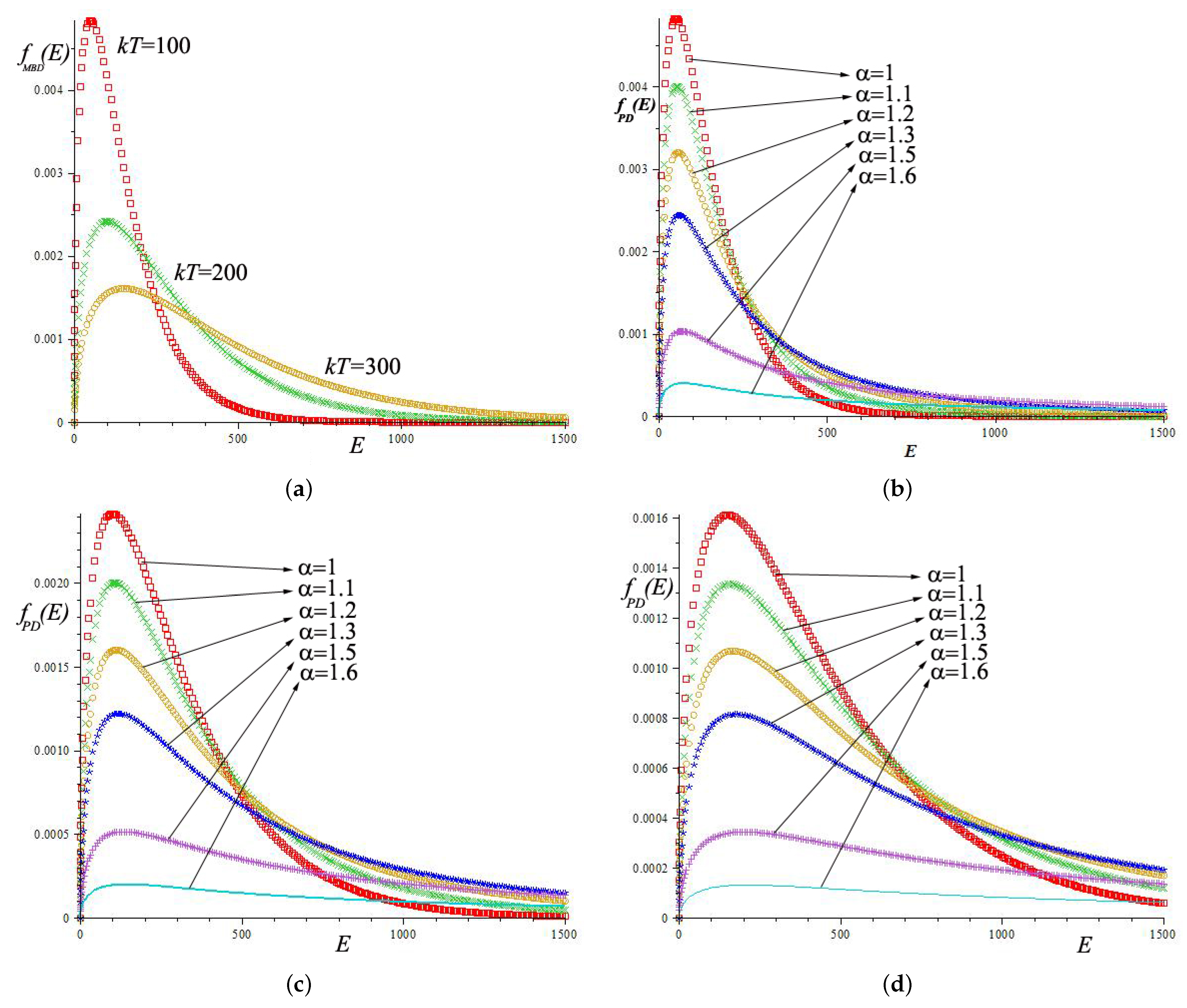
Figure 1a shows the Maxwell–Boltzmann energy distribution for the value of k T = 100 , 200 , 300 . As we increase the value of k T it is observed that the function is heavy tailed and less peaked. Figure 1b–d show the pathway distribution for k T = 100 , 200 , 300 , respectively. f P D ( E ) is plotted for α = 1 , α = 1.1 , α = 1.2 , α = 1.3 , α = 1.5 and α = 1.6 .
From the graphs, it can be observed that the pathway energy distribution ( f P D ( E ) ) is more general than the Maxwell–Boltzmann energy distribution ( f M B D ( E ) ). We can retrieve the Maxwell–Boltzmann energy distribution from pathway distribution as α 1 . As we increase the value of k T in f P D ( E ) we observe that the function becomes thinker-tailed and the peak is reduced.

5. Conclusions

An attempt has been made to change the energy distribution of the ions in the plasma from the Maxwell–Boltzmann case. By this change of using the pathway energy distribution, more unstable and chaotic situations are covered, whereas the standard Maxwell–Boltzmann situation is retrieved by letting α 1 . It may be noted that even a small deviation of the energy distribution with α produces dramatic effects on those nuclear reaction rates whose main contribution comes from the high energy tail of the distribution which can be observed from the Figure. The extended non-resonant thermonuclear functions in the Maxwell–Boltzmann and cut-off case were already obtained in the paper of Haubold and Kumar [1,2] by using the single variable Mellin transform technique. Here, the standard and extended non-resonant thermonuclear functions with depleted tail are evaluated by using the two variable Mellin transform technique which helped to obtain more convenient closed form representations. It is first time ever in the literature the two variable Mellin transform technique and the two variable H-function are utilized to obtain closed form representations of the thermonuclear functions. The generalization technique obtained here by means of the pathway model of Mathai provides a motivation to apply these technique to any other situation were similar circumstances arise, creating a more general class of solutions. The figures are plotted by using Maple 14 under Microsoft Windows XP platform.

Author Contributions

Conceptualization, D.K. and H.J.H.; methodology, D.K. and H.J.H.; software, D.K.; validation, D.K. and H.J.H.; formal analysis, D.K. and H.J.H.; investigation, D.K. and H.J.H.; resources, D.K. and H.J.H.; writing—original draft preparation, D.K. and H.J.H.; writing—review and editing, D.K. and H.J.H.; visualization, D.K.; supervision, H.J.H.; funding acquisition, D.K. Both authors have read and agreed to the published version of the manuscript.

Funding

This research received no external funding.

Institutional Review Board Statement

Not applicable.

Informed Consent Statement

Not applicable.

Data Availability Statement

The study do not report any data.

Acknowledgments

The authors would like to thank the unknown referee for the valuable suggestions which enabled to improve the presentation of the material in the revised form. The first author would like to thank the University of Kerala for providing the financial support under the project No. 1622/2021/UOK to complete this research work.

Conflicts of Interest

The authors declare no conflict of interest.

References

  1. Haubold, H.J.; Kumar, D. Extension of thermonuclear functions through the pathway model including Maxwell-Boltzmann and Tsallis distributions. Astropart. Phys. 2008, 29, 70–76. [Google Scholar] [CrossRef] [Green Version]
  2. Haubold, H.J.; Kumar, D. Fusion yield: Guderley modeland Tsallis statistics. J. Plasma Phys. 2011, 77, 1–14. [Google Scholar] [CrossRef] [Green Version]
  3. Mathai, A.M.; Haubold, H.J. Modern Problems in Nuclear and Neutrino Astrophysics; Academie-Verlag: Berlin, Germany, 1988. [Google Scholar]
  4. Mathai, A.M.; Haubold, H.J. Review of mathematical techniques applicable in astrophysical reaction rate theory. Astrophys. Space Sci. 2002, 282, 265–280. [Google Scholar] [CrossRef] [Green Version]
  5. Haubold, H.J.; John, R.W. On the evaluation of an integral connected with the thermonuclear reaction rate in closed-form. Astron. Nachrichten 1978, 299, 225–232. [Google Scholar] [CrossRef]
  6. Fowler, W.A. Experimental and theoretical nuclear astrophysics:the quest for the origin of the elements. Rev. Mod. Phys. 1984, 56, 149–179. [Google Scholar] [CrossRef] [Green Version]
  7. Haubold, H.J.; Mathai, A.M. Analytic representations of modified non-resonant thermonuclear reaction rates. J. Appl. Math. Phys. 1986, 37, 685–695. [Google Scholar] [CrossRef]
  8. Coraddu, M.; Kaniadakis, G.; Lavagno, A.; Lissia, M.; Mezzorani, G.; Quarati, P. Thermal distributions in stellar plasmas, nuclear reactions and solar neutrinos. Braz. J. Phys. 1999, 29, 153–168. [Google Scholar] [CrossRef]
  9. Fowler, W.A.; Caughlan, G.R.; Zimmerman, B.A. Thermonuclear rection rates. Annu. Rev. Astron. Astrophys. 1967, 5, 525–570. [Google Scholar] [CrossRef]
  10. Ferreir, C.; Lopez, J.L. Analytic expansions of thermonuclear reaction rates. J. Phys. A 2004, 37, 2637–2659. [Google Scholar] [CrossRef]
  11. Haubold, H.J.; Mathai, A.M. On thermonuclear reaction rates. Astrophys. Space Sci. 1998, 258, 185–199. [Google Scholar] [CrossRef]
  12. Eder, G.; Motz, H. Contribution of high-energy particles to thermonuclear reaction rates. Nature 1958, 182, 1140–1142. [Google Scholar] [CrossRef]
  13. Clayton, D.D.; Dwek, E.; Newman, M.J.; Talbot, R.J., Jr. Solar models of low neutrino counting rate: The depeted Mazwellian tail. Astrophys. J. 1975, 199, 494–499. [Google Scholar] [CrossRef] [Green Version]
  14. Erdélyi, A.; Magnus, W.; Oberhettinger, F.; Tricomi, F.G. Higher Transcendental Functions; McGraw-Hill: New York, NY, USA; Reprinted: Krieger, FL, USA, 1953; Volume I. [Google Scholar]
  15. Erdélyi, A. Asymptotic Expansions; Dover Publications: New York, NY, USA, 1956. [Google Scholar]
  16. Srivastava, H.M.; Gupta, K.C.; Goyal, S.P. The H-Functions of One and Two Variables with Applications; South Asian Publishers: New Delhi, Madras, 1982. [Google Scholar]
  17. Mathai, A.M.; Saxena, R.K. The H-Function with Applications in Statistics and Other Disciplines; Halsted Press [John Wiley & Son]: New York, NY, USA, 1978. [Google Scholar]
  18. Mathai, A.M. A Handbook of Generalized Special Functions for Statistics and Physical Sciences; Clarendo Press: Oxford, UK, 1993. [Google Scholar]
  19. Mathai, A.M.; Haubold, H.J. On generalized distributions and pathways. Phys. Lett. A 2008, 372, 2109–2113. [Google Scholar] [CrossRef] [Green Version]
  20. Mathai, A.M.; Saxena, R.K. Generalized Hypergeometric Functions with Applications in Statistics and Physical Sciences; Lecture Notes in Mathematics; Springer: Berlin/Heidelberg, Germany; New York, NY, USA, 1973; Volume 348. [Google Scholar]
  21. Fox, C. Some applications af Mellin transforms to the theory of bivariate statistical distributions. Proc. Camb. Philos. Soc. 1957, 53, 620–628. [Google Scholar] [CrossRef]
  22. Hai, N.T.; Yakubovich, S.B. The Double Mellin-Barnes Type Integrals and Their Applications to Convolution Theory; World Scientific Publishing: Singapore, 1992. [Google Scholar]
  23. Mathai, A.M. A pathway to matrix-variate gamma and normal densities. Linear Algebra Appl. 2005, 396, 317–328. [Google Scholar] [CrossRef] [Green Version]
  24. Mathai, A.M.; Haubold, H.J. Pathway model, superstatistics, Tsallis statistics and a generalized measure of entropy. Physics A 2007, 375, 110–122. [Google Scholar] [CrossRef] [Green Version]
  25. Gell-Mann, M.; Tsallis, C. (Eds.) Nonextensive Entropy: Interdisciplinary Applications; Oxford University Press: New York, NY, USA, 2004. [Google Scholar]
  26. Tsallis, C. Possible generalization of Boltzmann-Gibbs statistics. J. Stat. Phys. 1988, 52, 479–487. [Google Scholar] [CrossRef]
  27. Tsallis, C. Introduction to Non-Extensive Statistical Mechanics; Springer: New York, NY, USA, 2009. [Google Scholar]
  28. Beck, C.; Cohen, E.G.D. Superstatistics. Physics A 2003, 322, 267–275. [Google Scholar] [CrossRef] [Green Version]
  29. Mathai, A.M.; Haubold, H.J. On generalized entropy measures and pathways. Physics A 2007, 385, 493–500. [Google Scholar] [CrossRef] [Green Version]
  30. Kumar, D.; Haubold, H.J. On extended thermonuclear functions through pathway model. Adv. Space Res. 2009, 45, 698–708. [Google Scholar] [CrossRef] [Green Version]
Figure 1. (a) f M B D ( E ) for k T = 100 , 200 , 300 . (b) f P D ( E ) for k T = 100 , α = 1 , α = 1.1 , α = 1.2 , α = 1.3 , α = 1.5 and α = 1.6 . (c) f P D ( E ) for k T = 200 , α = 1 , α = 1.1 , α = 1.2 , α = 1.3 , α = 1.5 and α = 1.6 . (d) f P D ( E ) for k T = 300 , α = 1 , α = 1.1 , α = 1.2 , α = 1.3 , α = 1.5 and α = 1.6 .
Axioms 10 00115 g001
Publisher’s Note: MDPI stays neutral with regard to jurisdictional claims in published maps and institutional affiliations.

