Sparse 3D Seismic Imaging in the Kylylahti Mine Area, Eastern Finland: Comparison of Time Versus Depth Approach

Abstract

A 10.5 km² 3D seismic survey was acquired over the Kylylahti mine area (Outokumpu mineral district, eastern Finland) as a part of the COGITO-MIN (COst-effective Geophysical Imaging Techniques for supporting Ongoing MINeral exploration in Europe) project, which aimed at the development of cost-effective geophysical imaging methods for mineral exploration. The cost-effectiveness in our case was related to the fact that an active-source 3D seismic survey was accomplished by using the receiver spread originally designed for a 3D passive survey. The 3D array recorded Vibroseis and dynamite shots from an active-source 2D seismic survey, from a vertical seismic profiling experiment survey, as well as some additional “random” Vibroseis and dynamite shots made to complement the 3D source distribution. The resulting 3D survey was characterized by irregular shooting geometry and relatively large receiver intervals (50 m). Using this dataset, we evaluate the effectiveness of the standard time-imaging approach (post-stack and pre-stack time migration) compared to depth imaging (standard and specialized Kirchhoff pre-stack depth migration, KPreSDM). Standard time-domain processing and imaging failed to convincingly portray the first ~1500 m of the subsurface, which was the primary interest of the survey. With a standard KPreSDM, we managed to obtain a good image of the base of the Kylylahti formation bordering the extent of the mineralization-hosting Outokumpu assemblage rocks, but otherwise the image was very noisy in the shallower section. The specialized KPreSDM approach (i.e., coherency-based Fresnel volume migration) resulted in a much cleaner image of the shallow, steeply dipping events, as well as some additional deeper reflectors, possibly representing repetition of the contact between the Outokumpu assemblage and the surrounding Kalevian metasediments at depth.

1. Introduction

Mineral exploration using 2D seismic surveys is now more than three decades old [1]. The utilization of 3D seismics for deep mineral targeting started close to the beginning of this century [2] and since then several successful case studies have demonstrated the potential of 3D seismics to image geologically complex environments (e.g., [3,4,5,6,7,8,9] and the references therein). Near surface-heterogeneities, low signal-to-noise ratio and scattering of seismic waves are some of the key challenges in applying seismics in hardrock environment. Moreover, terrain accessibility typically restricts the optimal 3D survey design, which further creates challenges in processing and interpretation due to, e.g., coarse line spacing, inadequate offset and azimuth coverage as well as sparse and irregular geometries leading to significant acquisition footprints [4].

Hardrock seismic data processing needs to be tailored to meet the above challenges. Until recently, the most popular approach has been to apply partial pre-stack migration (dip moveout, DMO) followed by simple post-stack time migration (PoSTM). Pre-stack time migration (PreSTM) is not best suited for complex media, as it inherently assumes a local 1D velocity model. However, when applied to good quality, regular 3D data, it can produce significantly improved images as compared with the DMO-PoSTM approach (e.g., [10]). Pre-stack depth migration (PreSDM) is a standard routine in the oil and gas industry to tackle various imaging problems in the presence of strong subsurface heterogeneities. However, depth imaging in a hardrock environment is often hampered by the fact that conventional velocity model-building tools like reflection tomography or migration-velocity analysis [11] cannot be easily adopted due to the missing coherent reflections. Therefore, they cannot produce accurate velocity models required for migration. Nonetheless, there are some recent successful case studies of PreSDM application to image crystalline rocks in 3D (e.g., [12,13]). Those examples employed a specialized variants of Kirchhoff PreSDM called Fresnel volume migration (FVM) [14,15] or coherency-based FVM (CBFVM) [16] to reduce artefacts related to the migration operator and consequently improve image quality. Those methods are especially applicable and appealing in the case of sparse data, acquired using irregular shooting patterns, which is often the case for seismic investigations in hardrock settings.

In this paper, we evaluate the effectiveness of the standard time-imaging approach (DMO-PoSTM/PoSTM and PreSTM) in comparison to depth imaging (standard Kirchhoff PreSDM and CBFVM) using data from a 10.5-km² 3D seismic survey acquired over the Kylylahti mine area, located within the Outokumpu mineral district in eastern Finland. This dataset was acquired as a part of the COGITO-MIN project, which aimed at the development of cost-effective geophysical imaging methods for mineral exploration [17]. The cost-effectiveness in this case was related to the fact that we used the same receiver grid for the active source 3D survey which was originally designed for a 3D passive survey [18]. Moreover, acquisition of active-source 3D seismic data with regular source line geometry in a populated mining area with abundant lakes, swamps and other restrictions would not have been achievable. In such restricted areas, unconventional, tailored 3D survey geometries are the only option for executing an active-source 3D survey. Furthermore, as the sources form a major part of the costs of a 3D survey, the aim was to test if a sparse active-source 3D survey can provide a significantly cheaper alternative when the financial resources, terrain conditions or permissions do not allow for regular 3D source line geometries. The 3D array recorded Vibroseis and dynamite shots made for the 2D data acquisition [19], vertical seismic profiling (VSP) [20], as well as some additional “random” Vibroseis and dynamite shots made to complement the 3D source distribution. The resulting 3D survey is characterized by an irregular shooting geometry and relatively large receiver intervals (50 m). In this case, the PreSDM approach provided superior results to the PoSTM and PreSTM approaches in terms of imaging the ore-hosting Kylylahti formation.

This paper is organized as follows. In the “Materials and Methods” section, we discuss the geological background of the Kylylahti area, we describe the data acquisition and provide the basic theory behind CBFVM. The “Results” section is split into two parts: first, we present the basic time processing workflow and the time-domain imaging results. Subsequently, we show the depth imaging results, starting from velocity model building, standard Kirchhoff PreSDM and then the preferred CBFVM PreSDM approach. In the “Discussion” section, we provide some interpretation on the Kylylahti structure based on the 3D seismic data.

2. Materials and Methods

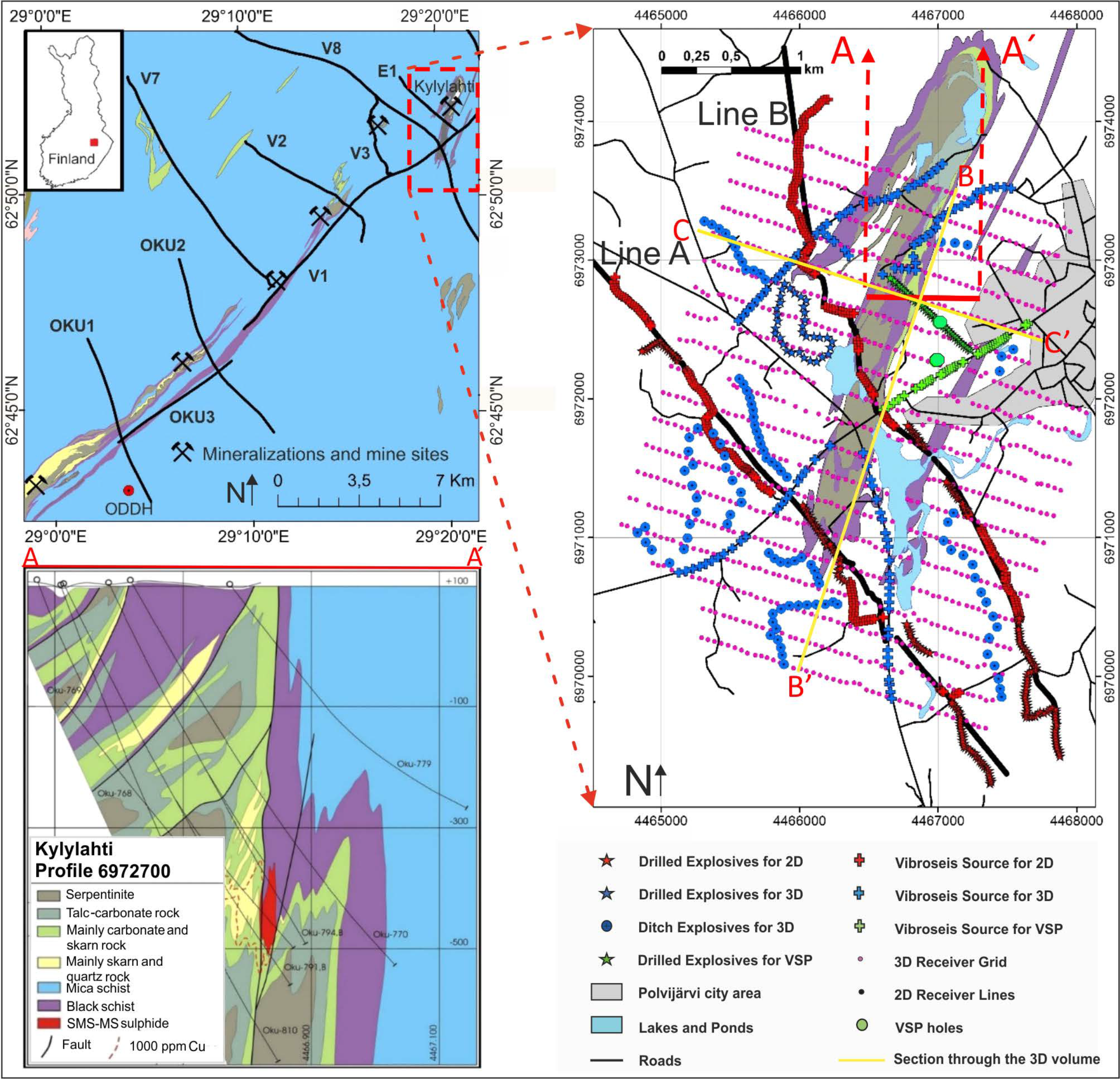
2.1. Geological Background

The Kylylahti polymetallic (Cu-Co-Zn-Ni-Ag-Au) semi-massive to massive sulphide ore deposit is situated in the famous Outokumpu mining district in eastern Finland. The Outokumpu ore belt comprises Paleoproterozoic turbiditic deep-water sediments and ophiolitic slices of upper mantle rocks from oceanic lithosphere forming the Outokumpu nappe. The Outokumpu nappe was thrusted from south-southwest onto the Archaean basement. Following the thrusting, two deformation phases took place. First, by a southeast–northwest compression which resulted in isoclinal recumbent folding. This is responsible for the thickening of Outokumpu ore [21]. The second folding buckled the existing folds into steeper but open antiforms and synforms. The deformation phases produced mainly N, NNE and NE trending upright folds. Due to deformation, the mantle-derived rocks were split into numerous pieces distributed in the upper crust. Metamorphic alteration changed the originally depleted upper mantle rocks into serpentinite–skarn–carbonate–quartz rocks [22,23]. The deposits are polymetallic (Cu-Co-Zn-Ni-Ag-Au) semi-massive to massive sulphide ores systematically hosted by the ophiolite-derived rock assemblage: the serpentinite–skarn–quartz rock association. These assemblages are typically enveloped by iron sulphide and graphite-bearing black schist.

During the past 100 years, the Outokumpu area has hosted several sulphide mines, but currently Boliden’s Kylylahti mine is the only operational sulphide mine in the area. The Kylylahti deposit comprises three north–northeast elongated semi-massive to massive sulphide lenses, with a total length of about 1.5 km, along a contact between carbonate—skarn—quartz rocks and black schists. In Kylylahti, the Outokumpu assemblage rocks (hereinafter referred to as Kylylahti formation) show multiple phases of deformation and strong foliations within a tight synformal fold structure, with the mineralization located along a near-vertical eastern limb (Figure 1). Because of the complex geometry, Kylylahti formation constitutes a difficult target for surface seismic methods. However, rock property measurements [24] indicate strong enough contrasts in acoustic impedances to produce a detectable reflected signal from contacts between the ore-bearing Outokumpu assemblage rocks and the surrounding black schists and turbiditic mica schists (Kalevian metasediments). Additionally, varying acoustic impedances for the Outokumpu assemblage rocks cause reflectivity from internal contacts between Outokumpu ultramafics: the talc-carbonate and serpentinite rock, and altered Outokumpu ultramafics: the carbonate–skarn–quartz rock association in the overall ore-bearing formation.

2.2. COGITO-MIN 3D Seismic Survey

The combined 3D passive/active seismic survey was performed in the Kylylahti mine area during August—September 2016. It was primarily designed to test body-wave reflections seismic interferometry, inspired by the pioneering study from Lalor Lake, Canada [27]. The survey layout includes 19 receiver lines spaced every 200 m with a receiver interval of 50 m (Figure 1). Six 10 Hz vertical-component geophones were bunched together at each receiver station and connected to a wireless recorder, resulting in a stationary spread of 994 active channels. Data were recorded quasi-continuously (20 h per day) with a 2 ms sampling interval for 30 days. During this period, other components of the COGITO-MIN survey took place, i.e., 2D seismic acquisition along two profiles (Line A and Line B) using both Vibroseis and dynamite sources [28] (Figure 1), and vertical seismic profiling (VSP) in underground boreholes, with dedicated Vibroseis and dynamite sources also on the surface [20]. In order to improve source density and create a sparse 3D active-source survey to benchmark results of seismic interferometry, additional Vibroseis and explosive sources were placed wherever permitted (Figure 1). Apart from a group of explosives detonated in drillholes, some charges were also fired in the ditches. Altogether, the 3D survey comprised 738 shot points. The main survey acquisition parameters are listed in

Table 1. Main acquisition parameters of COGITO-MIN 3D seismic survey.

Survey Parameters
Recording System	OYO 1-Geospace GSR 2
No. of Receiver Lines	19 lines
Receiver Line Interval	200 m
Receiver (group) Interval	50 m
Number of Receivers	994
Survey Area	~10.5 km2
Geophones	10 Hz (string of 6, bunched), GS-20
Shot Spacing	20–100 m
Number of Shot Points	738
CDP 3 Bin Size	25 × 25 m
Explosive Source	120–240 g charge in 2 m drilled hole or ditch
Vibroseis Source	2 × INOVA 4 UniVibe trucks (9.5t)
Sweep Parameters/No. of Sweeps	4–220 Hz, 16 s/3 (2D) 3–200 Hz, 20 s/2 (3D random) 30–220 Hz, 16 s/6, low force (VSP) 10–300 Hz, 10 s/6, low force (VSP)
Spread Configuration	Fixed spread, continuous recording
Record Length	6 s
Sampling Interval	2 ms

¹ OYO Geospace Company; ² Geospace Seismic Recorder; ³ Common Depth Point; ⁴ INOVA Geophysical Company.

.

Shot gathers were extracted from the continuous data using recorded GPS time-stamps. Vibroseis records were correlated with the pilot sweep and vertically stacked. The data quality observed in the raw shot gathers is variable: the best quality data are from 2D/3D Vibroseis shots and drilled explosives. Poor quality data resulted from the VSP Vibroseis shots, probably due to the vibrator low-force and single-vibe operations. First breaks are usually observed up to the maximum offset of around 5 km but sometimes it is difficult to correlate them due to the coarse receiver spacing of 50 m. In the complex geological setting, hardly any coherent shallow reflections are identified in the raw shot gathers. On the other hand, deeper reflections (~2 s two-way traveltime) can be clearly distinguished in the raw shot gathers. Figure 2 shows a comparison of data recorded from co-located Vibroseis and dynamite shot. While the dynamite shot exhibits a broader frequency bandwidth (both at low and high frequency ends), the Vibroseis record has a better signal-to-noise ratio (SNR), due to the stacking of multiple sweeps. In the Vibroseis record, there are also hints of a shallow reflection event at 0.3–0.4 s (indicated by arrows in Figure 2b).

2.3. Basic Theory of the Specialized Kirchhoff Pre-Stack Depth Migration

Kirchhoff PreSDM (KPreSDM) is based on the integral solution of the wave equation in the form of the diffraction stack integral [29]. It can be written as:

$$\mathrm{V}\left(i\right)=\frac{-1}{2\mathsf{\pi }}\underset{\mathrm{A}}{{\displaystyle \iint }}\mathrm{w}\left(i,r\right)·\dot{\mathrm{u}}\left(r,{\mathrm{t}}_{\mathrm{s}}+{\mathrm{t}}_{\mathrm{r}}\right)\mathrm{dr}$$

(1)

where V represents the solution of the Kirchhoff integral which is given by the weighted sum over the diffraction surface A. Here i = i(x,y,z) is the image point, ${\mathrm{t}}_{\mathrm{s}}$ is the traveltime from source to the image point, ${\mathrm{t}}_{\mathrm{r}}$ is the traveltime from image point to the receiver, $\dot{\mathrm{u}}$ is the time derivative of the wavefield and r is the distance from image point to the receiver. V is an image value for an arbitrary image point (i) in the subsurface. The function w(i,r) represents a weighting term of the amplitudes along the diffraction curve (${\mathrm{t}}_{\mathrm{s}}+{\mathrm{t}}_{\mathrm{r}}$) and accounts for the directivity and amplitude loss due to spherical divergence. The time derivative of the wavefield $\dot{\mathrm{u}}$ is integrated using this weighting term over the aperture A along the diffraction surface (${\mathrm{t}}_{\mathrm{s}}+{\mathrm{t}}_{\mathrm{r}}$) and yields the image value V. The same process is performed for each point in the subsurface.

To further improve the KPreSDM technique, two additional weighting factors: f(i,r) and ${\mathrm{C}}^{\mathrm{p}}\left(i,r\right)$ can be added which will be dependent on the actual image point (i) and the receiver location (r) as shown in Equation (2).

$$\mathrm{V}\left(i\right)=\frac{-1}{2\mathsf{\pi }}\underset{\mathrm{A}}{{\displaystyle \iint }}\mathrm{f}\left(i,r\right)·{\mathrm{C}}^{\mathrm{p}}\left(i,r\right)·\mathrm{w}\left(i,r\right)·\dot{\mathrm{u}}\left(r,{\mathrm{t}}_{\mathrm{s}}+{\mathrm{t}}_{\mathrm{r}}\right)\mathrm{dr}$$

(2)

One way of implementing the weighting term f(i,r) in the depth domain is by using FVM [15] which restricts the migration operator to the physically relevant part along the two-way traveltime isochrones as shown in Equation (3). In order to do so, first the emergent angle of the wavefield at the receiver is determined for each time sample of the recorded trace. A local slowness analysis is performed e.g., by a slant-stack technique, which is based on the coherency of the wavefield in order to obtain a reliable emergent angle in the case of single component data. A semblance coefficient is evaluated in a time window around each sample to be migrated and is used as an additional weighting factor within the Kirchhoff integral. In the second step, a ray is back propagated into the subsurface in the direction of the emergent angle as an initial condition. Furthermore, a paraxial Fresnel volume is constructed along this ray and the migration operator is restricted to this Fresnel volume. The Fresnel volume itself includes all the image points whose two-way traveltime is less than ${\mathrm{t}}_{\mathrm{s}}+{\mathrm{t}}_{\mathrm{r}}$ plus half the dominant time period of the source signal T.

$$\mathrm{f}\left(i,r\right)=\left\{\begin{array}{ccc}1& \mathrm{if}& \mathrm{d}\le {\mathrm{r}}_{\mathrm{f}}\\ \frac{\mathrm{d}-\sqrt{2}{\mathrm{r}}_{\mathrm{f}}}{{\mathrm{r}}_{\mathrm{f}}\left(1-\sqrt{2}\right)}& \mathrm{if}& {\mathrm{r}}_{\mathrm{f}}<\mathrm{d}<\sqrt{2}{\mathrm{r}}_{\mathrm{f}}\\ 0& \mathrm{if}& \mathrm{d}\ge \sqrt{2}{\mathrm{r}}_{\mathrm{f}}\end{array}\right\}$$

(3)

Here, d is the orthogonal distance from the image point to the ray and ${\mathrm{r}}_{\mathrm{f}}$ is the radius for the Fresnel volume taken into account. The weighting term equals 1 within the first Fresnel volume. It is tapered between the first and second Fresnel volume and is set to zero outside of the Fresnel volume.

The second weighting term is incorporated to further suppress the random, incoherent noise in the data by taking advantage of the nearby receivers. The weighting factor is computed as a semblance coefficient which is defined as the ratio of coherent to total energy within a time window over a certain number of neighboring traces. Mathematically it can be written as in Equation (4) [30,31].

$${\mathrm{C}}^{\mathrm{p}}\left(i,r\right)={\left(\frac{{\int }_{-\mathrm{T}/2}^{\mathrm{T}/2}{\left|{\sum }_{\mathrm{j}=0}^{\mathrm{N}-1}{\mathrm{u}}_{\mathrm{j}}\left({\mathrm{t}}_{\mathrm{s}}+{\mathrm{t}}_{{\mathrm{r}}_{\mathrm{j}}}+\mathrm{t}\right)\right|}^2\mathrm{dt}}{\mathrm{N}{\int }_{-\mathrm{T}/2}^{\mathrm{T}/2}{\left|{\sum }_{\mathrm{j}=0}^{\mathrm{N}-1}{\mathrm{u}}_{\mathrm{j}}\left({\mathrm{t}}_{\mathrm{s}}+{\mathrm{t}}_{{\mathrm{r}}_{\mathrm{j}}}+\mathrm{t}\right)\right|}^2\mathrm{dt}}\right)}^{\mathrm{p}}$$

(4)

As the semblance coefficient is a normalized value, ranging from 0 to 1, it can be directly used as an additional weighting factor in the Kirchhoff integral. The resulting image depends upon three parameters: the value of exponent p, the number of neighboring traces N and the time window length T. The most important parameter on which the result largely depends is the number of neighboring traces taken into account and the aperture spanned by the receivers. For this reason, it is beneficial to define a maximum offset distance between the source and the corresponding receivers for the semblance coefficient calculation instead of a fixed number of traces. This approach is much more relevant for surveys with irregular geometry. Therefore, an approximated first Fresnel zone radius is computed for each image point as per Equation (5).

$${\mathrm{r}}_{{\mathrm{F}}_{\mathrm{pro}}}=\sqrt{\left({\mathrm{dx}}^2+{\mathrm{dy}}^2+{\mathrm{dz}}^2\right)}\sqrt{2\frac{{\mathrm{t}}_{\mathrm{dom}}}{{\mathrm{t}}_0}}\sqrt{\frac{{\mathrm{dx}}^2+{\mathrm{dy}}^2}{{\mathrm{dz}}^2}+1}$$

(5)

The first term shows the distance of the image point i(x,y,z) to the receiver (r), ${\mathrm{t}}_{\mathrm{dom}}$ denotes the dominant time period of the source signal and ${\mathrm{t}}_0$ equals twice the traveltime between the image point and the receiver (${\mathrm{t}}_0=2{\mathrm{t}}_{\mathrm{r}}$). The first and second term combined represents the radius to the Fresnel zone approximation. The third term represents the projection of the paraxial Fresnel zone to the surface. By computing Equation (5), we are computing the second local boundary condition for the maximum distance to the comparison traces. If the computed traveltimes coincide with the observed two-way traveltimes of a recorded arrival, the semblance window aligns around the recorded arrival and yields a high-semblance value. In contrast, a low-semblance value is obtained when the computed traveltimes do not match the observed two-way traveltimes. The traveltimes from the source and receiver locations to the image points are calculated using a finite difference solution of the eikonal equation [32]. For more details, readers are referred to [16].

3. Results

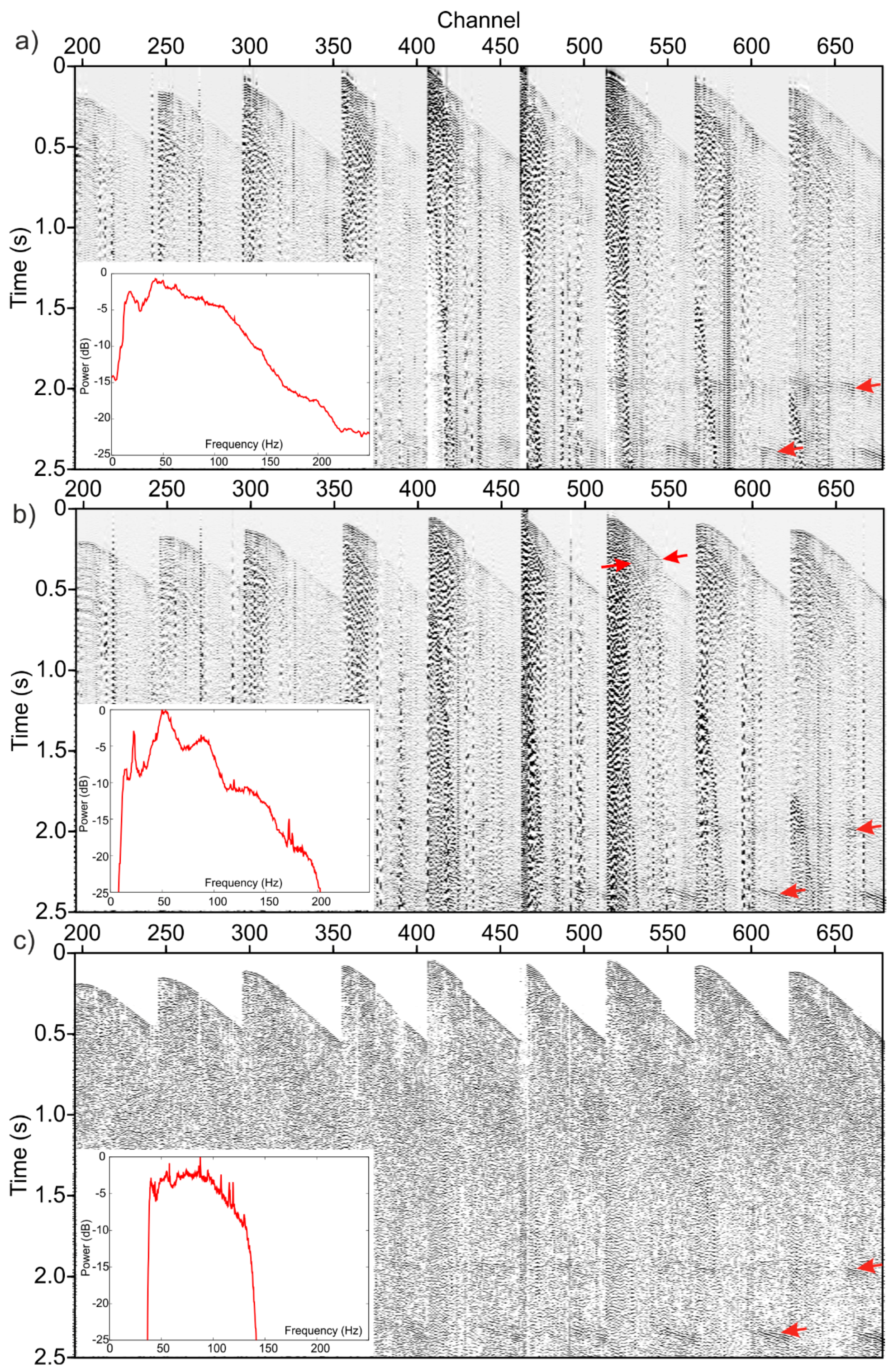
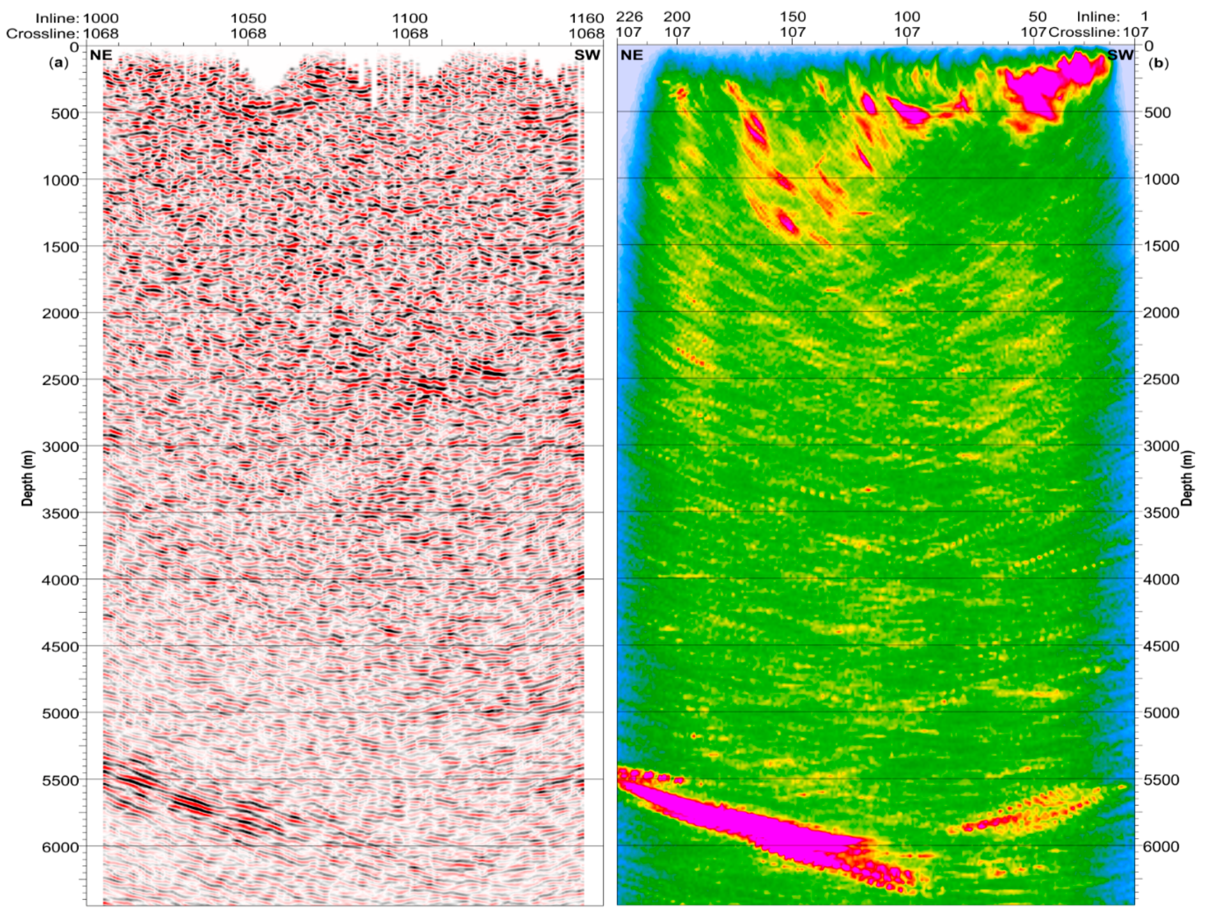
3.1. Data Processing and Time-Domain Imaging

The data processing employed procedures typically used in processing hardrock seismic data. Our processing sequence is summarized in

Table 2. Processing steps for COGITO-MIN 3D survey (dip moveout–post-stack time migration (DMO–PoSTM/PoSTM)).

Process	Parameter
1. First-Stage Processing Flow
Data read	3.0 s SEG–Y 1 data
Match Filter	Match dynamite to Vibroseis
Geometry	3D, 25 × 25 m bins
Refraction Statics	2-layer model, replacement velocity 5000 m/s
Fixed Datum	100 m above sea level
Geometrical Spreading Compensation	v2t function
Amplitude Balance	Surface consistent, 0-2 s window
Notch Removal	50/100 Hz
Deconvolution	Single Trace Predictive, filter length 80 ms–gap 14 ms
Airwave mute	330 m/s
Band-pass Filter	35-40-130-150 Hz
AGC 2	250 ms
Top Mute	30 ms below V = 5500 m/s
2a. First Approach
Residual Statics Analysis	3 passes
Velocity Analysis	2 passes
NMO 3 corrections	with 2nd pass velocities
Top Mute	angle mute 35 degrees
Stack	Sqrt-fold normalization
2b. Second Approach
DMO corrections	3D Kirchhoff DMO
Velocity analysis	1 pass
Top mute	angle mute 35 degree
Stack	Sqrt-fold normalization
3. Migration and Post-Processing
Migration	3D Stolt, V = 5400 m/s
Coherency Filter	F-XY Decon. 3IL × 3XL 100 ms window
Band-pass Filter	20-30-95-105 Hz
Trace Balance	Whole Trace Balance
Resampling	4 ms
Time-Depth Conversion	V = 5400 m/s or tomography
Output Data	SEG-Y

¹ Standard data storage format from Society of Exploration Geophysicists (SEG); ² Automatic Gain Control; ³ Normal moveout.

. Because of the irregular shot lines and the variable shot spacing (20–100 m) along the lines, we decided to use square bins of 25 × 25 m during the geometry setup. A special emphasis has been put in the refraction statics based on a two-layer model using the first break picks for the full offset range. In a hardrock environment setting, the near-surface low-velocity layer can have a significant impact on the misalignment of the reflections. To calculate the refraction statics, close to half a million traces were handpicked.

Ground roll and direct shear wave energy was mostly attenuated using band-pass filtering (compare raw and processed shot in Figure 2b,c). A single trace predictive deconvolution, with an operator length of 80 ms and a gap length of 14 ms, was found most effective in enhancing shallow reflectivity. Normal moveout (NMO) correction was carried out with two passes of velocity analysis done on every fifth inline and crossline. Stacking velocities were in the range of 5300–6500 m/s. After the two passes of velocity and residual statics analysis, three different approaches were performed to obtain final migrated stacks. In the first approach, a final NMO stack was migrated using 3D Stolt migration (PoSTM) with a constant velocity of 5400 m/s (combination of steps 2a and 3 in Table 2). We chose the velocity of 5400 m/s based on processing of COGITO-MIN 2D seismic data [28]. In case of 2D data, this velocity provided better fit between mapped geological contacts at the surface and the migrated reflections. Also, the same velocity had been applied during the processing of the legacy HIRE (High Resolution Reflection Seismics for Ore Exploration 2007–2010) data [33]. In the second approach, a 3D integral DMO was applied before PoSTM. This involved another pass of velocity analysis on the gathers after the DMO correction (see step 2b in Table 2). The third approach employed PreSTM. After some initial testing, no velocity analysis was performed on the migrated gathers. PreSTM was tested using both the final NMO velocity model and the post-DMO velocities.

The reflectivity observed in all the approaches down to the depths of ~1200 m is generally incoherent (Figure 3), although the extent of these piece-wise continuous reflectors are co-relatable when investigated in the whole area (Figure 4). There is a zone of increased reflectivity between 2000–3000 m depth, which continues up dip. A strong reflection package is observed at ~4500–5000 m depth.

3.2. Depth-Domain Imaging

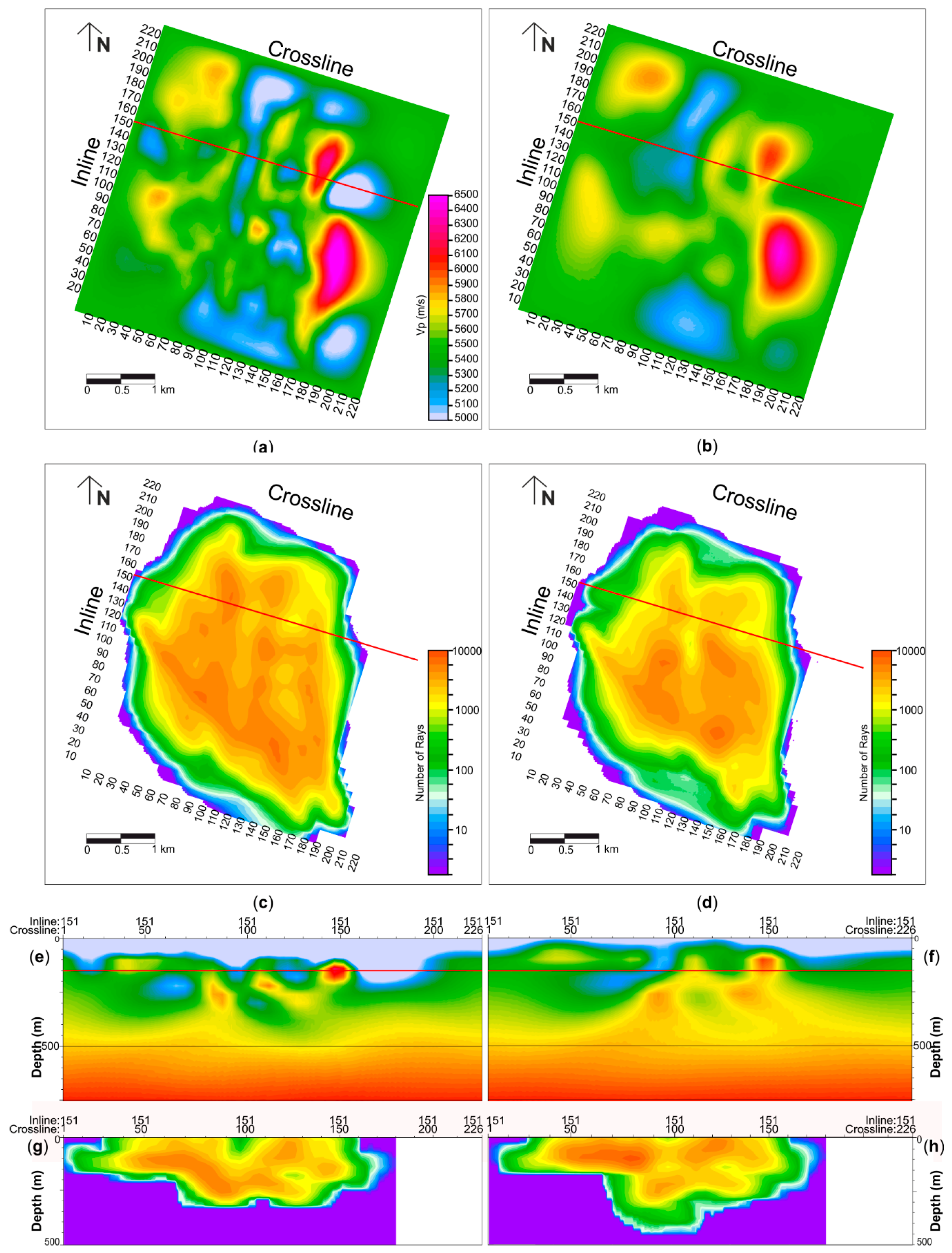
3.2.1. Velocity Model Building

The quality of depth imaging depends on the ability to derive a reliable interval velocity model. Earlier attempts to perform depth migration with a constant velocity model produced substantially degraded images for the target depths. Since the coherency of reflections in the Kylylahti area is very low, standard reflection tomography is not applicable. Therefore, we performed first-arrival traveltime tomography (FAT) to derive the velocity model using the FAST package [34]. Close to 380,000 handpicked first breaks were used in the inversion. A grid with cubic 20 × 20 × 20 m cells was used for traveltimes calculations in the forward modelling step. The inversion was parameterized on a grid with 100 × 100 × 40 m cells. We used two approaches in running FAT. In the first approach, we run tomography with the raw picks. In the second approach, before running the inversion, we corrected the picks by the same refraction statics as applied during data processing. The idea behind the second approach is to correct for the thin near-surface weathering layer, which is producing traveltime shifts and, which cannot be accurately modelled unless a very fine model discretization is used. This could also be resolved during FAT with an additional statics term being calculated simultaneously with the model update during the inversion [7,35], however, such an approach was not attempted here. Instead, we followed a simpler approach by just correcting the picks before inversion. In both cases, the inversion was run with 3 non-linear iterations and up to 7 iterations of testing the trade-off parameter between the data fit and model smoothness [34]. A normalized misfit value of 1 is expected once the inversion is complete, which means that the data fitting is within the picking uncertainty. In the first approach, the normalized misfit value dropped from ~9 to ~2.5 (Root-mean square (RMS) traveltime residual of ~8 ms). In the second approach, the normalized misfit value dropped from ~10 to ~1 (RMS traveltime residual of ~5 ms). As expected, the picks corrected by refraction statics resulted in better convergence. Figure 5 shows the comparison of velocity model built from both approaches and ray-density coverage through a depth slice at 150 m depth (below the datum of 100 m above the sea level) and a vertical cross-section along the inline marked by red line in Figure 5a,b. Figure 5a,b shows the P-wave velocity model built using FAT with raw picks and picks corrected using refraction statics, respectively. The corresponding ray-density coverage maps associated with both models are shown in Figure 5c (raw picks) and Figure 5d (picks corrected with refraction statics). The vertical cross-section along the inline position is illustrated in Figure 5e,f with respective ray-density plots in Figure 5g,h. The models appear quite different, with short-scale perturbations in case of the model built from the raw picks. This means that the near-surface anomalies are affecting the recovery of the bedrock velocities. Ray-coverage map relates directly to the source locations. From Figure 5e,f, it can be deduced that the meaningful velocity perturbations are observed down to a maximum depth of ~500–600 m, however the majority of rays reach as deep as 300 m only. There is a slightly better ray penetration in case of the FAT run with the corrected picks (reaching 450 m depth), which can be probably attributed to the smoother velocity model, which is preventing the rays from channeling at localized velocity contrasts.

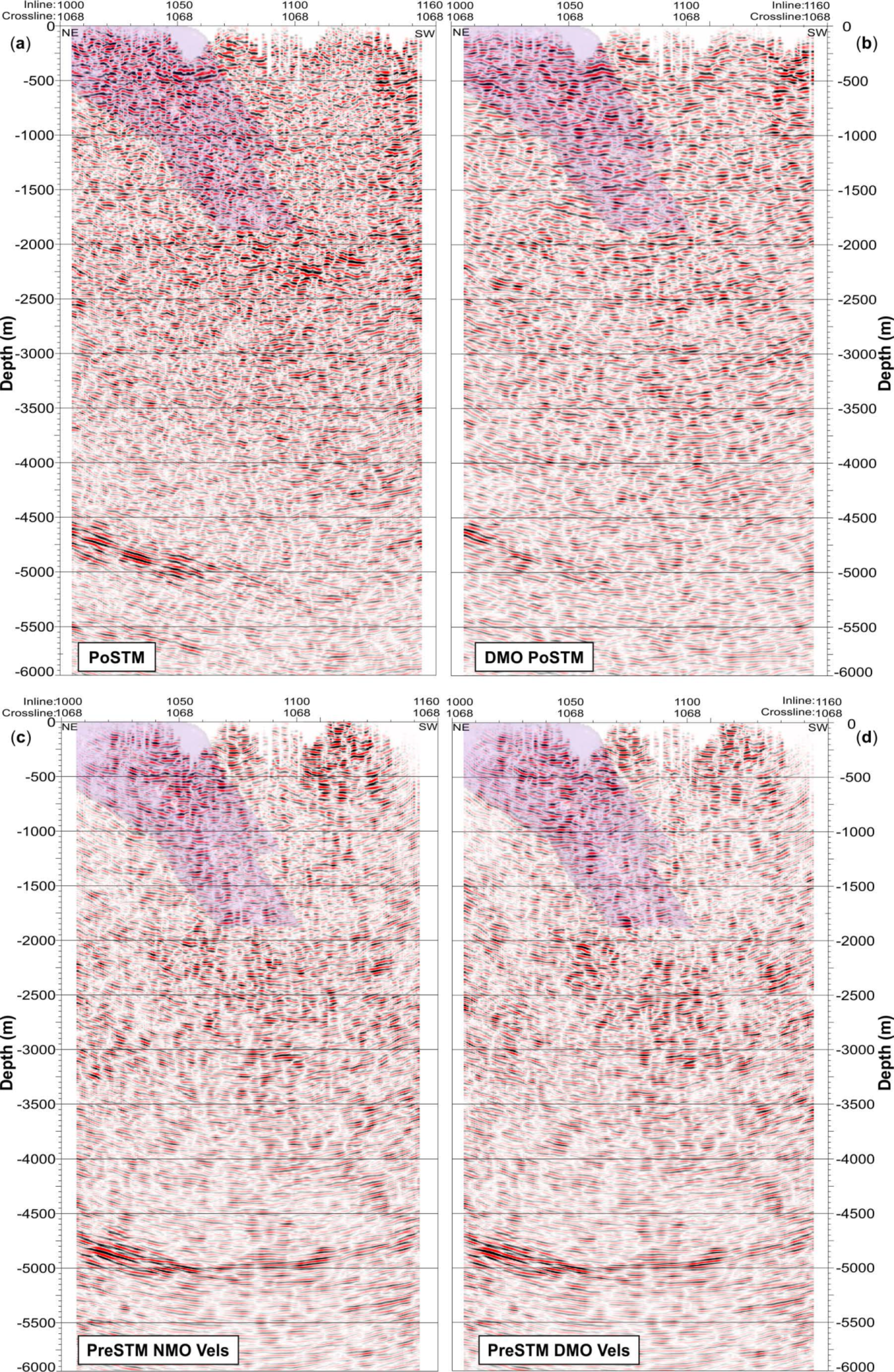
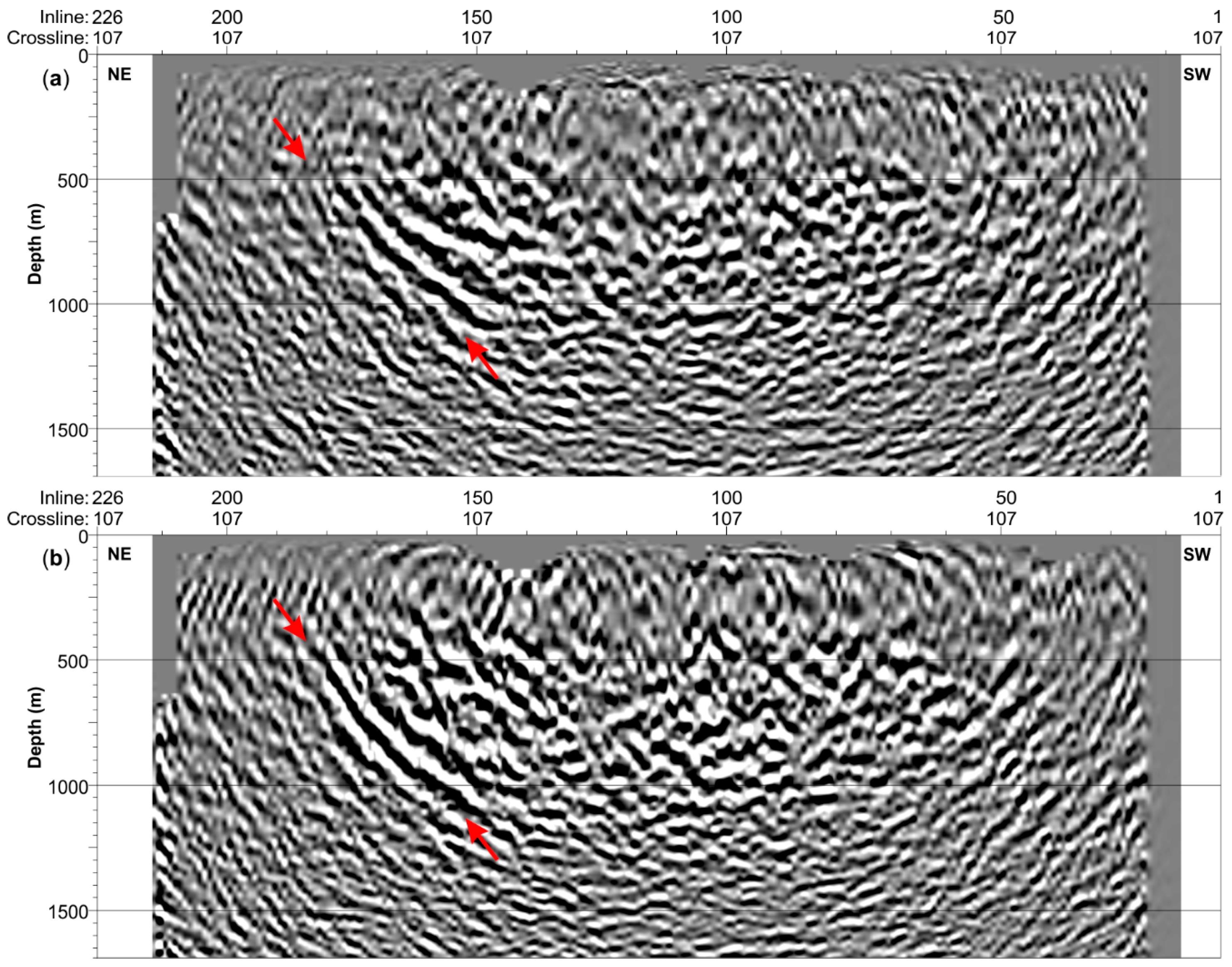
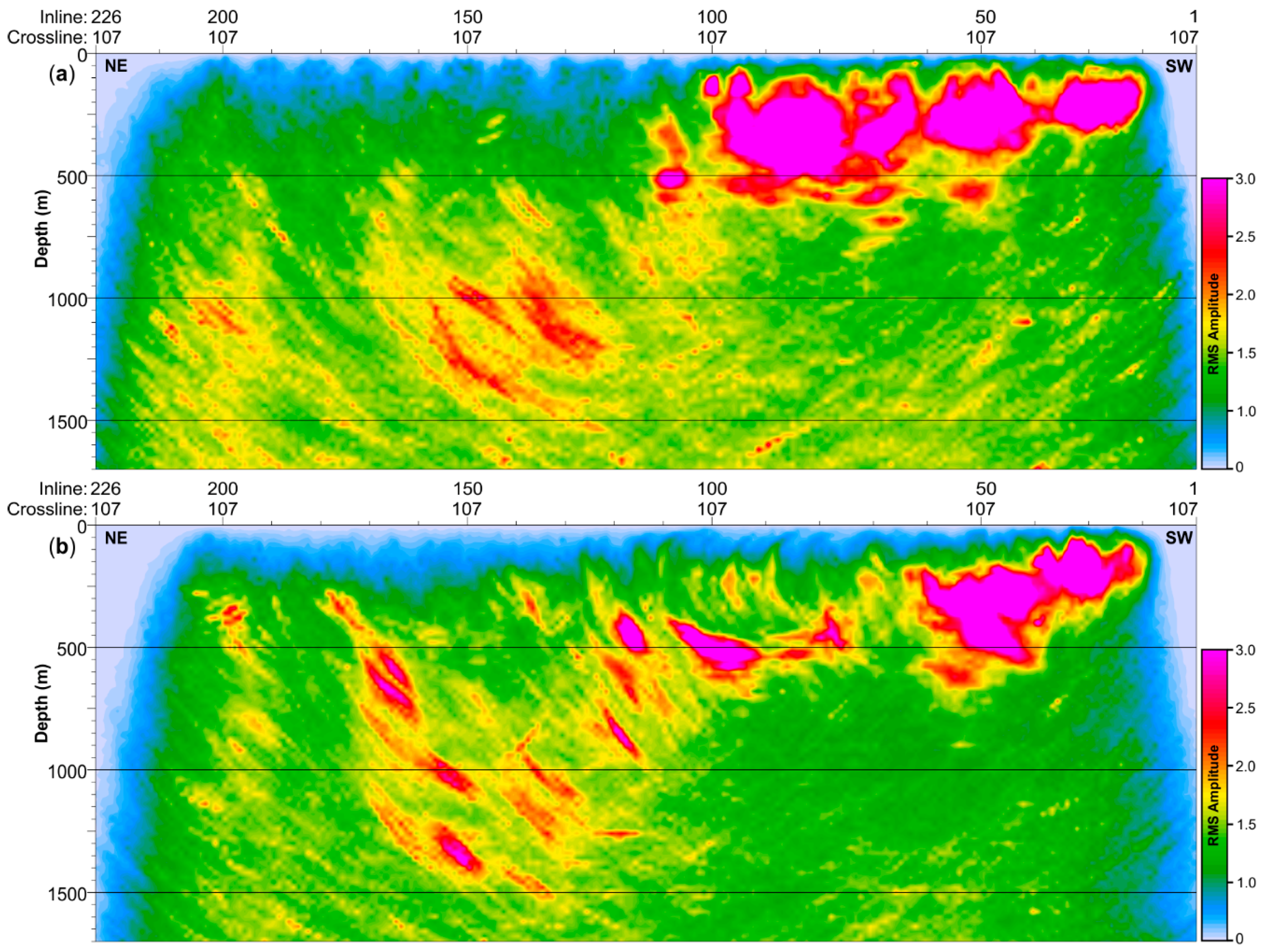
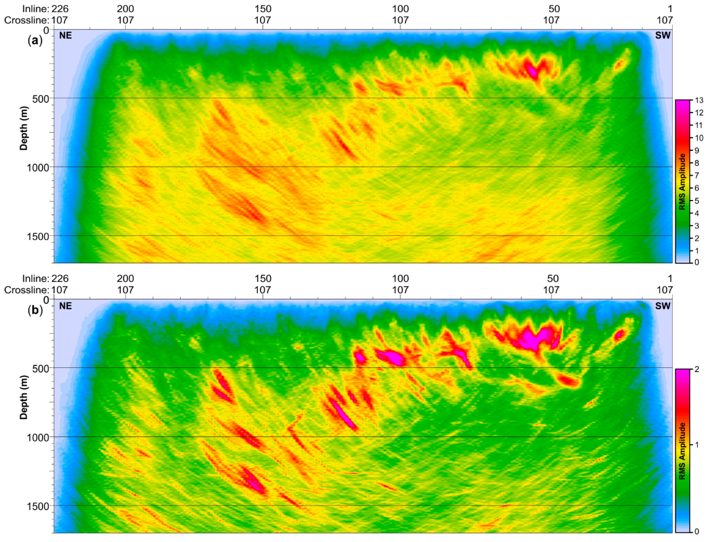
3.2.2. Standard Kirchhoff Pre-Stack Depth Migration (KPreSDM)

The first approach used for the depth imaging was KPreSDM. It was run using an industry-standard algorithm (TSUNAMI software by Tsunami Development, Inc. based in Houston, Texas, USA) operating on common-offset planes and producing standard common-image gathers (CIG). The input to migration was the same as for PreSTM, except for the application of residual statics. CIGs were produced every 100 m for offsets between 0 to 5000 m. After some testing, we used the full aperture defined by 90-degree angle of the migration operator (from vertical) and 3000 m distance. An anti-alias filter was also applied to the operator to improve imaging of steep dips. Migration was performed with traveltimes calculated using the velocity models discussed above. We retained the original velocity model parameterization (20 × 20 × 20 m cells) and, therefore, we output the CIGs at 20 × 20 m bins (which differs from the binning used for time imaging). It turned out that the velocity model build with the picks corrected for refraction statics resulted in an image which is better focused (compare sections in Figure 6) and better positioned at depth, as verified against borehole-derived constraints (see Section 4). Migrated CIGs were subjected to post-processing including a coherency and band-pass filter, as well as an angle mute before stacking. An f-k filter suppressing sub-horizontal artefacts was run on the stacked volume. Figure 6 shows the results of KPreSDM.

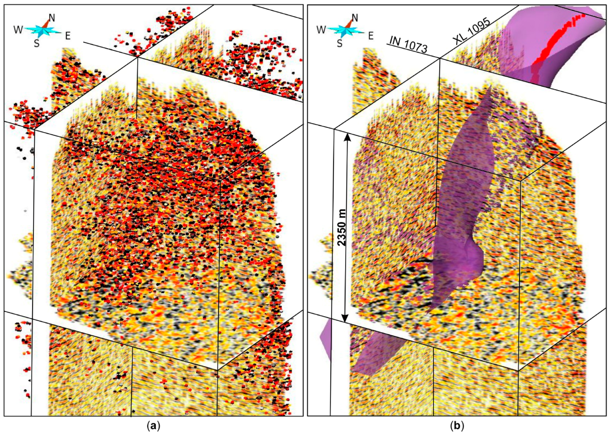
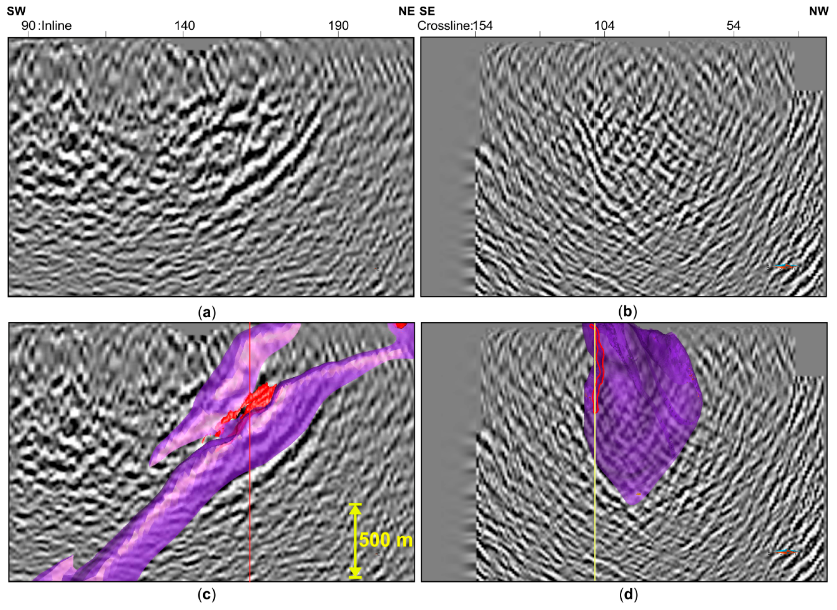
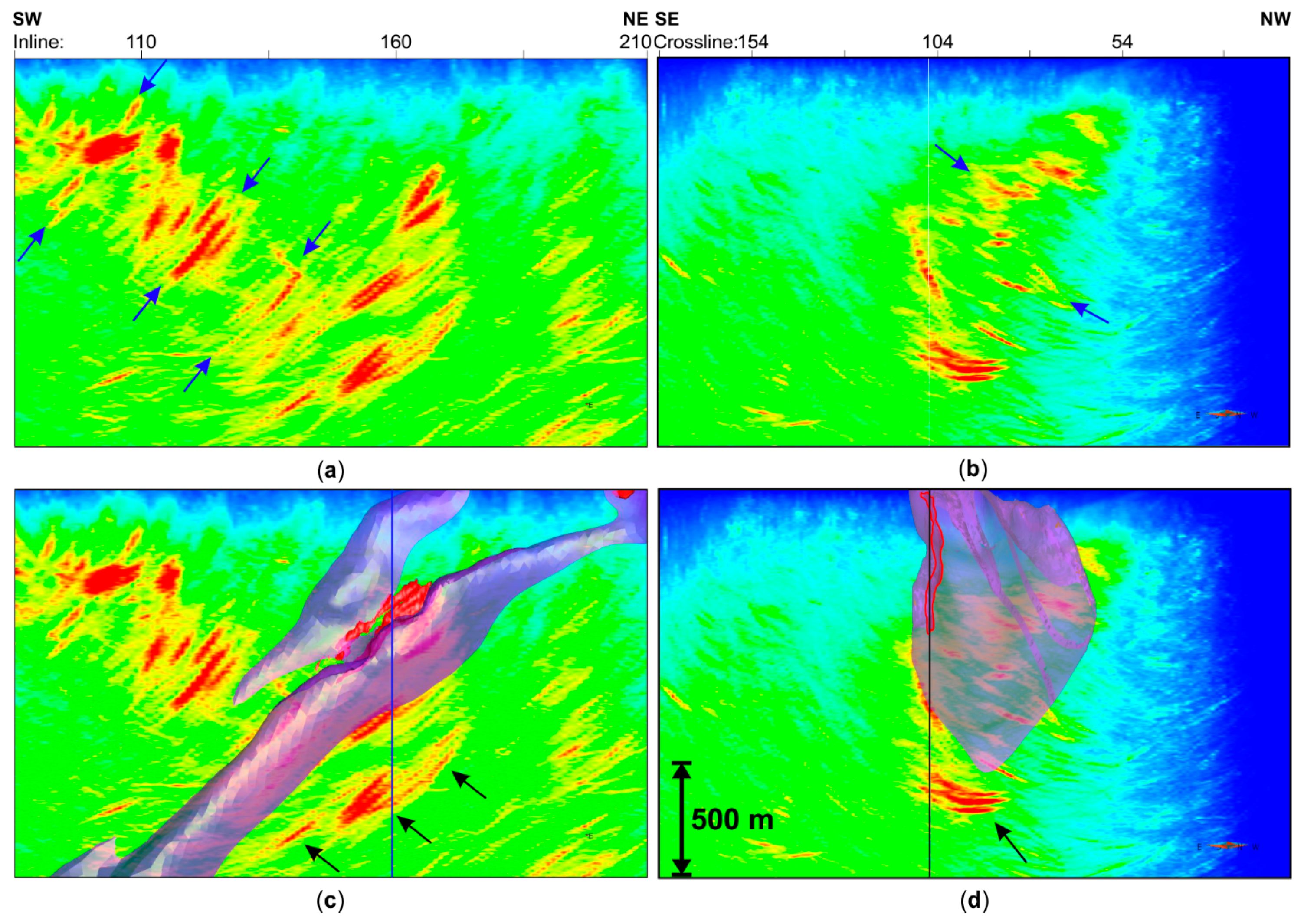
3.2.3. Specialized Kirchhoff PreSDM

Encouraged by the imaging results of the KPreSDM as compared to the time imaging, we investigated if the specialized form of KPreSDM, i.e., CBFVM as described in Section 2.3, can bring further improvements. After some initial testing with the constant velocity model, we concluded that qualitatively best results are obtained from CBVFM among other approaches (e.g., FVM alone). This was also suggested by previous studies performed in crystalline environments (e.g., [12,13,16,30]). Therefore, here we focus on the results of the CBFVM approach.

Similar to KPreSDM, we tested two velocity models. Initially, the migration volume was sampled at 20 × 20 × 20 m, i.e., the same sampling as the velocity model (Figure 7). Having relatively coarse vertical sampling reduced the computational time, which is significantly higher for the CBFVM (~26hrs on 96 cores using 20 m vertical sampling) as compared to the KPreSDM (2 h on 48 cores using 5 m vertical sampling). The main overhead is related to the additional ray-tracing performed in the FVM, as well as the slowness calculation. There are several parameters that need to be set in CBFVM. The most important ones are related to the semblance calculation (Equation (4)). We computed the semblance coefficient for the estimation of emergent angle using 21 receiver traces. Then, we used a maximum offset distance of 290 m (circular radius), and a maximum of neighboring receivers set to 27 in order to determine the weighting for each image point. While taking into account the actual dominant frequency content in the data close to ~40 Hz, we tested different values of dominant frequencies ranging from 40 to 100 Hz, but the lower dominant frequencies did not bring much improvements in the results. So we decided to use 0.01 s as the preferred dominant time period in our case (Equation (5)). Also, as discussed earlier, result depends on the power value “p” (Equation (4)), and therefore we also tested two different values of p = 1 and p = 2 (Figure 8).

The input data were the same as for KPreSDM, i.e., time-preprocessed data as prepared for PreSTM, except for the residual statics. Unlike the KPreSDM implementation used in Section 3.2.2, which is acting on common-offset planes and producing CIGs, our implementation of CBFVM is run on shot gathers. The resulting migrated shot gathers are stacked. No muting or other post-processing was applied. A root-mean square of the amplitudes is computed before stacking.

It is clear from Figure 7 that the CBFVM run using the velocity model build with the picks corrected with refraction statics is superior in terms of image focusing. Therefore, the velocity model built with the corrected picks was considered as preferred one for further testing. In the CBFVM run with the velocity model built from the raw picks, migration noise is appearing between inlines 1–100 down to 500 m depth (Figure 7a). It might be due to the presence of high velocity contrast in the shallow section and higher density of shots with a spacing of 20 m (shots used in 2D acquisition). Based on single shot analysis and considering the contribution of each shot to the image, it appears that the noise can be heavily reduced by skipping a few of the shots during stacking which are not contributing significantly in the target area. However, at the same time we will lose image quality in other parts of the area, so it is a trade-off between number of shots and imaging of the reflectors. We changed the migration grid interval to 5 m (as in KPreSDM) and tested the semblance exponent values (Equation (4)). A value of p = 2 (Figure 8b) is enhancing the coherent signal much more effectively than the p = 1 version (Figure 8a). This is probably due to the fact that the reflections present in our data are very weak. On the other hand, taking a very large “p” value might create some artefacts, so we decide not to further increase it. However, it is worth noting the significance of choosing different grid dimensions for migration and its effect on depth imaging results (compare Figure 7b and Figure 8b). The migration noise has been significantly reduced in the upper ~500 m.

4. Discussion

One of the main anticipated outcomes of the COGITO-MIN 3D survey was a better understanding of the complex geological setting and imaging of the steeply dipping and tightly folded Kylylahti formation with a sparse and irregular shooting pattern. It is clear from Figure 9a that down to depth of ~1500 m the time-domain approach (PoSTM) failed to provide a convincing image of the Kylylahti structure, showing only sparse piece-wise continuous reflectivity. On the other hand, these sparse reflections are trackable in a 3D volume and can be used as a proxy to delineate the overall extent of the Kylylahti formation (Figure 4). On the contrary, the CBFVM results (Figure 9b) show abundant reflectivity in the shallower section, with dips in agreement with the expected geological structure. However, deeper down, there is an increase in reflectivity between 2000 to 3000 m depth observed in the PoSTM (Figure 9a), followed by a more transparent zone. This may represent deeper extension of the Outokumpu assemblage rocks, as indicated by the regional HIRE profiles [17,33]. Such increased subhorizontal reflectivity is absent in the CBFVM image (Figure 9b). A coherent southwest-dipping reflective package can be tracked in the depth range of 5200 to 6000 m in both imaging versions, likely representing the mafic dykes on top of the Archean basement as confirmed earlier from the regional HIRE profiles (e.g., [33]).

Focusing more on the first ~1500 m, we can use available geological constraints, i.e., extensive drillhole data and the geological model provided by Boliden for seismic data interpretation. This model was primarily based on the drillhole data, but includes constraints from results obtained by electromagnetic and potential field methods. In Figure 10, a crossline and an inline from the KPreSDM performed with the velocity model built with the picks corrected using refraction statics (same as in Figure 6b) are shown. When we compare seismic data with the surface representing the contact of the ophiolite sequence (Outokumpu assemblage rocks) with the black schists (i.e., the base of the Kylylahti formation), we can note a very good correlation with a proper depth positioning of reflectors, indicating that the velocity model used for migration was appropriate. The eastern flank of the formation (Figure 10b,d) is better imaged when compared to the western flank. It is probably due to the survey layout, i.e., both the receiver line extension and the shot locations with respect to the dip of the strata. The city of Polvijärvi is located in the east (Figure 2), so no shot points were allowed there. The reflectivity pattern shows no clear correlation with the projected model of semi-massive to massive ore (red surface in Figure 10c,d).

The CBFVM image (Figure 11) is much cleaner, as noise produced due to migration and sparse coverage has been heavily reduced. There are coherent, steeply dipping reflectors present at shallower depths (Figure 11a, blue arrows), which are obscured in the KPreSDM results (Figure 10). However, a shorter segment of the Kylylahti formation base is imaged (Figure 11) when compared with the KPreSDM (Figure 10), both along the crossline and inline direction. The flanks of the formation are not easy to interpret when looking at the inline (compare Figure 10b,d with Figure 11b,d); apart of the imaging of a short segment of the eastern flank, bright reflectivity is confined within an area enveloped by the surface representing a contact between the Outokumpu assemblage rocks and surrounding black schists (Figure 11b,d). Those reflectors can be attributed to the complex internal architecture of the Kylylahti formation. Similar to the KPreSDM, there is no clear correlation of the reflectors with the projected ore deposit model (red surface in Figure 11c,d). Although, it is worth noting the smearing of the reflectors along the inline direction (Figure 11b, blue arrows). This might be due to the fact that the weighting for each image point is being calculated using semblance coefficient within a circular distance. A large crossline spacing of 200 m results in less contribution in the crossline direction as compared to more number of geophones in the inline direction. Hence, larger weighting in the inline direction is smearing the reflectors in that direction. Interestingly, some reflectors with hints of increased reflectivity at depth visible in the time imaging (Figure 9a), occurring ~300 m below the base of the ophiolite sequence (marked by black arrows in Figure 11) are not observed in the KPreSDM. At present the origin of these deeper reflectors has not been verified as no boreholes are drilled to reach these depths. One possible explanation is that it is a repetition of the Outokumpu assemblage rocks and the surrounding Kalevian metasediments at depth. They can also be related to sulphide-bearing black schist interlayers within mica schists.

5. Conclusions

Three-dimensional seismic reflection data were acquired with a sparse and irregular source pattern in the Kylylahti polymetallic mining and exploration area in eastern Finland to explore the depth extent of lithologies hosting the mineralization. We evaluated the effectiveness of the standard time-imaging approach (DMO-PoSTM/PoSTM and PreSTM) in comparison to depth imaging including industry-standard KPreSDM, as well as CBFVM. Standard time-domain processing and imaging failed to convincingly portray the first ~1500 m, which are the primary target depths of the survey. With KPreSDM, we managed to obtain a good image of the contact of the ophiolite rocks (Outokumpu assemblage) with the black schists (i.e., the base of the Kylylahti formation), but otherwise the image was very noisy in the shallower section. The CBFVM approach resulted in a much cleaner image of the shallow subsurface, including steeply dipping reflectors, as well as with some additional deeper reflectors below the known extent of the Outokumpu rocks. However, the base of the Kylylahti formation was more visible in the KPreSDM. This proves that both the standard (KPreSDM) and specialized pre-stack depth imaging (CBFVM) provide complementary information and can be highly beneficial in hardrock seismic exploration in case of the complex geological setting such as the Kylylahti deposit and/or sparse data.

References

1. Reed, L.E. Seismic Reflection Surveying for Mining Exploration Applications. A Review of Practice Past and Current with an Outlook for the Future, Toronto, Mineral Industry Technology Council of Canada (MI-TEC) Report. 1993; 219p, Unpublished.
2. Milkereit, B.; Berrer, E.K.; King, A.R.; Watts, A.H.; Roberts, B.; Adam, E.; Eaton, D.W.; Wu, J.; Salisbury, M.H. Development of 3-D seismic exploration technology for deep nickel-copper deposits—A case history from the Sudbury basin, Canada. Geophysics 2000, 65, 1890–1899. [Google Scholar] [CrossRef]
3. Bellefleur, G.; Cheraghi, S.; Malehmir, A. Reprocessing legacy three-dimensional seismic data from the Halfmile Lake and Brunswick No. 6 volcanogenic massive sulphide deposits, New Brunswick, Canada. Can. J. Earth Sci. 2018. [Google Scholar] [CrossRef]
4. Cheraghi, S.; Malehmir, A.; Bellefleur, G. 3D imaging challenges in steeply dipping mining structures: New lights on acquisition geometry and processing from the Brunswick no. 6 seismic data, Canada. Geophysics 2012, 77, WC109–WC122. [Google Scholar] [CrossRef]
5. Koivisto, E.; Malehmir, A.; Hellqvist, N.; Voipio, T.; Wijns, C. Building a 3D model of lithological contacts and near-mine structures in the Kevitsa mining and exploration site, Northern Finland: Constraints from 2D and 3D reflection seismic data. Geophys. Prospect. 2015, 63, 754–773. [Google Scholar] [CrossRef]
6. Malehmir, A.; Bellefleur, G. 3D seismic reflection imaging of volcanic-hosted massive sulfide deposits: Insights from reprocessing Halfmile Lake data, New Brunswick, Canada. Geophysics 2009, 74, B209–B219. [Google Scholar] [CrossRef]
7. Malehmir, A.; Tryggvason, A.; Wijns, C.; Koivisto, E.; Lindqvist, T.; Skyttä, P.; Montonen, M. Why 3D seismic data are an asset for exploration and mine planning? Velocity tomography of weakness zones in the Kevitsa Ni-Cu-PGE mine, northern Finland. Geophysics 2017, 83, B33–B46. [Google Scholar] [CrossRef]
8. White, D.J.; Secord, D.; Malinowski, M. 3D seismic imaging of volcanogenic massive sulfide deposits in the Flin Flon mining camp, Canada: Part 1—Seismic results. Geophysics 2012, 77, WC47–WC58. [Google Scholar] [CrossRef]
9. White, D.J.; Malinowski, M.; Devine, C.; Gilmore, K.; Schetselaar, E.; Pehrsson, S. Drill Targeting with 3-D Seismics for Volcanogenic Massive Sulfide Exploration in the Flin Flon Mining Camp. Econ. Geol. 2016, 111, 903–912. [Google Scholar] [CrossRef]
10. Bellefleur, G.; Schetselaar, E.; White, D.; Miah, K.; Dueck, P. 3D seismic imaging of the Lalor volcanogenic massive sulphide deposit, Manitoba, Canada. Geophys. Prospect. 2015, 63, 813–832. [Google Scholar] [CrossRef]
11. Jones, F. Velocities, Imaging and Waveform Inversion: The Evolution of Characterising the Earth’s Subsurface; EAGE: Warsaw, Poland, 2018; p. 259. ISBN 978-94-6282-253-5. [Google Scholar]
12. Hloušek, F.; Buske, S. Fresnel Volume Migration of the ISO89-3D data set. Geophys. J. Int. 2016, 207, 1273–1285. [Google Scholar] [CrossRef]
13. Schreiter, L.; Hloušek, F.; Hellwig, O.; Buske, S. Characterization of seismic reflections from faults in a crystalline environment, Schneeberg, Germany. Geophys. Prospect. 2015, 63, 1015–1032. [Google Scholar] [CrossRef]
14. Lüth, S.; Buske, S.; Giese, R.; Goertz, A. Fresnel volume migration of multicomponent data. Geophysics 2005, 70, S121–S129. [Google Scholar] [CrossRef]
15. Buske, S.; Gutjahr, S.; Sick, C. Fresnel volume migration of single-component seismic data. Geophysics 2009, 74, WCA47–WCA55. [Google Scholar] [CrossRef]
16. Hloušek, F.; Hellwig, O.; Buske, S. Improved structural characterization of the Earth’s crust at the German Continental Deep Drilling Site using advanced seismic imaging techniques. J. Geophys. Res. Solid Earth 2015, 120, 6943–6959. [Google Scholar] [CrossRef]
17. Koivisto, E.; Malinowski, M.; Heinonen, S.; Cosma, C.; Wojdyla, M.; Vaittinen, K.; Chamarczuk, M.; Riedel, M.; Kukkonen, I.; The COGITO-MIN Working Group. From Regional Seismics to High-Resolution Resource Delineation: Example from the Outokumpu Ore District, Eastern Finland. In EAGE 2nd Conference on Geophysics for Mineral Exploration and Mining; Extended Abstract, Tu 2MIN P04; EAGE: Porto, Portugal, 2018. [Google Scholar]
18. Chamarczuk, M.; Malinowski, M.; Draganov, D.; Koivisto, E.; Heinonen, S.; Juurela, S.; Group, C.-M.W. Seismic Interferometry for Mineral Exploration: Passive Seismic Experiment over Kylylahti Mine Area, Finland. In EAGE 2nd Conference on Geophysics for Mineral Exploration and Mining; Extended Abstract, Tu 2MIN 03; EAGE: Porto, Portugal, 2018. [Google Scholar]
19. Heinonen, S.; Malinowski, M.; Hloušek, F.; Gislason, G.; Koivisto, E.; Buske, S.; The COGITO-MIN Working Group. Seismic Exploration in The Kylylahti Cu-Au-Zn Mining Area: Comparison of Time and Depth Imaging Approaches. In EAGE 2nd Conference on Geophysics for Mineral Exploration and Mining; Extended Abstract, Tu 2MIN P01; EAGE: Porto, Portugal, 2018. [Google Scholar]
20. Riedel, M.; Cosma, C.; Enescu, N.; Koivisto, E.; Komminaho, K.; Vaittinen, K.; Malinowski, M. Underground Vertical Seismic Profiling with Conventional and Fiber-Optic Systems for Exploration in the Kylylahti Polymetallic Mine, Eastern Finland. Minerals 2018, 8, 538. [Google Scholar] [CrossRef]
21. Koistinen, T.J. Structural evolution of an early Proterozoic strata-bound Cu-Co-Zn deposit, Outokumpu, Finland. Earth Environ. Sci. Trans. R. Soc. Edinb. 1981, 72, 115–158. [Google Scholar] [CrossRef]
22. Säntti, J.; Kontinen, A.; Sorjonen-Ward, P.; Johanson, B.; Pakkanen, L. Metamorphism and Chromite in Serpentinized and Carbonate-Silica-Altered Peridotites of the Paleoproterozoic Outokumpu-Jormua Ophiolite Belt, Eastern Finland. Int. Geol. Rev. 2006, 48, 494–546. [Google Scholar] [CrossRef]
23. Peltonen, P.; Kontinen, A.; Huhma, H.; Kuronen, U. Outokumpu revisited: New mineral deposit model for the mantle peridotite-associated Cu-Co-Zn-Ni-Ag-Au sulphide deposits. Ore Geol. Rev. 2008, 33, 559–617. [Google Scholar] [CrossRef]
24. Luhta, T. Petrophysical Properties of the Kylylahti Cu-Au-Zn Sulphide Mineralization and Its Host Rocks. Masters’ Thesis, University of Helsinki, Helsinki, Finland, 2019. [Google Scholar]
25. Bedrock of Finland—DigiKP Digital Map Database, Version 2.1; Geological Survey of Finland: Espoo, Finland, 2019; Available online: https://gtkdata.gtk.fi/Kalliopera/index.html (accessed on 29 March 2019).
26. Kontinen, A.; Peltonen, P.; Huhma, H. Description and Genetic Modelling of the Outokumpu-Type Rock Assemblage and Associated Sulphide Deposits; Final Technical Report for GEOMEX J.V., Workpackage “Geology”; Geological Survey of Finland: Espoo, Finland, 2006; Available online: http://tupa.gtk.fi/raportti/arkisto/m10_4_2006_1.pdf (accessed on 17 May 2019).
27. Cheraghi, S.; Craven, J.A.; Bellefleur, G. Feasibility of virtual source reflection seismology using interferometry for mineral exploration: A test study in the Lalor Lake volcanogenic massive sulphide mining area, Manitoba, Canada. Geophys. Prospect. 2015, 63, 833–848. [Google Scholar] [CrossRef]
28. Heinonen, S.; Malinowski, M.; Hloušek, F.; Gislason, G.; Buske, S.; Koivisto, E.; Wojdyla, M. Cost-Effective Seismic Exploration: 2D Reflection Imaging at the Kylylahti Massive Sulfide Deposit, Finland. Minerals 2019, 9, 263. [Google Scholar] [CrossRef]
29. Schneider, W.A. Integral formulation for migration in two and three dimensions. Geophysics 1978, 43, 49–76. [Google Scholar] [CrossRef]
30. Hloušek, F.; Hellwig, O.; Buske, S. Three-dimensional focused seismic imaging for geothermal exploration in crystalline rock near Schneeberg, Germany. Geophys. Prospect. 2015, 63, 999–1014. [Google Scholar] [CrossRef]
31. Neidell, N.S.; Taner, M.T. Semblance and other Coherency measures for Multichannel data. Geophysics 1971, 36, 482–497. [Google Scholar] [CrossRef]
32. Podvin, P.; Lecomte, I. Finite difference computation of traveltimes in very contrasted velocity models: A massively parallel approach and its associated tools. Geophys. J. Int. 1991, 105, 271–284. [Google Scholar] [CrossRef]
33. Kukkonen, I.T.; Heinonen, S.; Heikkinen, P.J.; Sorjonen-Ward, P. Delineating ophiolite derived host rocks of massive sulfide Cu-Co-Zn deposits with 2D high-resolution seismic reflection data in Outokumpu, Finland. Geophysics 2012, 77, WC213–WC222. [Google Scholar] [CrossRef]
34. Zelt, C.A.; Barton, P.J. 3D seismic refraction tomography: A comparison of two methods applied to data from the Faeroe basin. J. Geophys. Res. 1998, 103, 7187–7210. [Google Scholar] [CrossRef]
35. Tryggvason, A.; Schmelzbach, C.; Juhlin, C. Traveltime tomographic inversion with simultaneous static corrections—Well worth the effort. Geophysics 2009, 74, WCB25–WCB33. [Google Scholar] [CrossRef]
Figure 1. Location of the Kylylahti mine in the Outukumpu belt (top left) (Figure from “Bedrock of Finland—DigiKP Digital Map Database”; please see reference for full description [25]). Acquisition geometry of the COGITO-MIN 3D seismic survey (right panel). A-A’ is a cross-section through the Kylylahti deposit (bottom left) [26]. Yellow lines B-B’ and C-C’ mark a representative crossline and inline location, respectively, of the 3D seismic volume. This crossline and inline are used to showcase the imaging results. Labels show 2D profiles acquired within the same project (Line A and Line B).
Minerals 09 00305 g001
Figure 2. Comparison of shot gathers from a co-located dynamite and Vibroseis shot. Inset shows respective frequency spectra. (a) dynamite; (b) Vibroseis; (c) same as (b) but with full processing applied (without top mute), please see Table 2. Arrows point to some shallow and deep reflections. Note that the dynamite record was filtered to match the waveform of the Vibroseis record.
Minerals 09 00305 g002
Figure 3. Comparison of various time imaging approaches for crossline 1068 running along the ore zone (see Figure 1 for location). (a) PoSTM, (b) DMO followed by PoSTM, (c) pre-stack time migration (PreSTM) with final normal moveout (NMO) velocities, (d) PreSTM with post-DMO velocities. The known extent of the Kylylahti formation as modelled using borehole constraints by Boliden is shown in purple.
Minerals 09 00305 g003
Figure 4. Fence diagram showing time imaging results extracted from the PoSTM volume along inline 1073, crossline 1095 and a depth slice at 2350 m depth: (a) geobodies extracted from the maximum amplitude; (b) Kylylahti mineralization (in red) and the interpreted base of the Kylylahti formation (in purple) based on seismic data. Figure shows spatial extent of the increased, piece-wise continuous reflectivity characterizing the Kylylahti formation.
Minerals 09 00305 g004
Figure 5. Comparison of first-arrival traveltime tomography (FAT) velocity models and ray-density coverage. Depth slice at 150 m below the datum from: (a) P-wave velocity model built from raw picks; (b) P-wave velocity model built from picks corrected with refraction statics; (c) ray-density coverage map for (a); (d) ray-density coverage map for (b); inline 151 from: (e) P-wave velocity model shown in (a); (f) P-wave velocity model shown in (b); (g) ray-density for (e); (h) ray-density for (f). It can be observed that the model built from additional statics correction is smoother, has higher ray-density coverage and a greater ray extension in depth with respect to the model built from raw picks.
Minerals 09 00305 g005
Figure 6. Crossline along the ore zone from Kirchhoff pre-stack depth migration (KPreSDM) using the velocity model build with (a) raw picks; (b) picks corrected with refraction statics. Note the better focusing in (b) and the extent of the dipping reflector shown by red arrows.
Minerals 09 00305 g006
Figure 7. Crossline along the ore zone from the coherency-based Fresnel volume migration (CBFVM) run with 20 m vertical sampling using the velocity model build with (a) raw picks; (b) picks corrected with refraction statics. A semblance exponent p = 2 was used. Note: the velocity model built from FAT has the uniform sampling of 20 m in each direction.
Minerals 09 00305 g007
Figure 8. Crossline along the ore zone from the CBFVM run with 5 m vertical sampling using velocity model build with picks corrected with refraction statics and semblance exponent (a) p = 1, (b) p = 2 (compare with Figure 7b).
Minerals 09 00305 g008
Figure 9. Comparison of the time vs. depth imaging results along a crossline through the ore zone (see Figure 1 for location). (a) PoSTM; (b) CBFVM for velocity model with refraction statics applied (same as in Figure 7b). Note that the same velocity model was used for depth conversion of PoSTM.
Minerals 09 00305 g009
Figure 10. Crossline (a) and inline (b) extracted from the KPreSDM; (c) and (d) shows the data overlaid with the modelled base (from the borehole data) of the Kylylahti formation (in violet) and Kylylahti ore bodies (in red). See Figure 1 for location of the sections. The red line in (c) shows the inline position and yellow line in (d) shows the corresponding crossline position.
Minerals 09 00305 g010
Figure 11. Crossline (a) and inline (b) extracted from the CBFVM sampled at 5 m (same version as in Figure 8b); (c,d) shows the data overlaid with the modelled base (from the borehole data) of the Kylylahti formation (in violet) and Kylylahti ore bodies (in red). See Figure 1 for location of the sections. The red line in (c) shows the inline position and yellow line in (d) shows the corresponding crossline position. The blue line in (c) shows the inline position and the black line in (d) shows the corresponding crossline position.
Minerals 09 00305 g011