Breakage Characteristics of Heat-Treated Limestone Determined via Kinetic Modeling

Abstract

In recent years, heat treatment has attracted attention as a means to improve the color sorting technology with the aim of improving the quality of low-grade limestone. The crucial stage in this technique is to evaluate the breakage characteristics of the sample materials after color sorting. In this study, the breakage characteristics of samples showing color differences after heat treatment and of the original raw material were investigated using a laboratory ball mill. The grinding was characterized using the population balance model. Specific rates of breakage and the primary breakage distribution were experimentally determined by first-order kinetic plots and the BII method. The breakage parameters were also back-calculated by employing a simplex method. Grinding of the three materials indicated first-order kinetics, and the experimental results were well described by the model with parameters obtained by back-calculating.

1. Introduction

Limestone has approximately 300 different reported uses and can be processed into a variety of products. Cement and steel industries account for a high percentage of this usage, and in Korea, the steel and cement industries are the largest consumers of limestone. The material that has the greatest influence on the quality of limestone is CaO, and the refining of low-grade limestone is becoming an important issue as high-grade limestone reserves are depleted. In general, the low-grade limestone produced in Korea contains dolomite (MgCO₃), silica (SiO₂) and clay minerals, so its CaO content is relatively low. Since the basic characteristics (low activity and inhomogeneity) of the raw materials are also less favorable, it is difficult to apply them to high value-added industries, e.g., in steelmaking and fine chemical processes.

Improvement of low-grade limestone quality is generally accomplished through mineral processing. In particular, the crushing/grinding process has a low efficiency especially when the enormous amount of energy consumed is considered. As such, increasing the grinding efficiency will reduce energy consumption. To accomplish this, appropriate mill selection and operation at optimum milling conditions are necessary [1].

The crushing properties of limestone have been previously studied by many researchers. Deniz [2] used an impact crusher and investigated the grinding characteristics of three types of limestone with size distribution modelling using t-family curves. Nitta [3] and Deniz [4] analyzed the grinding characteristics of limestone in various mills using a typical Bond Index. Dundar and Benzer [5] conducted ball milling of raw materials such as cement clinker, pozzolan, blast furnace slag, limestone and gypsum within the same mill (also known as intergrinding). They observed that the fineness of each component cannot be individually controlled, resulting in over-grinding of relatively softer components. In addition, several studies have focused on the pulverization characteristics of smaller limestone particles using typical fine-grinding equipment such as a jet mill [6] and planetary mill [7]. Many researchers have also introduced a mathematical grinding model to study limestone [8,9,10].

In this study, the dolomite crystals in limestone were calcined by heat treatment into CaO, and the difference in the grinding rates between the materials was analyzed to improve the limestone grade. In particular, these improvements can be maximized through optical separation based on material color differences after calcination. The most important point in this process is to evaluate the grinding characteristics of each mineral sample that shows a color difference after calcination. The breakage characteristics of heat-treated limestone were determined using a laboratory ball mill. Mathematical modeling based on the mass balance equation and simulation of the grinding process using two functions—corresponding to the specific rate of breakage and primary breakage distribution—were performed. Using these two functions, the particle size of the ground product can be calculated at certain grinding times, and the production rate and particle size distribution can also be predicted for the grinding/classification circuit.

2. Theory

Specific Rate of Breakage and Primary Breakage Distribution

The kinetic grinding model consists of a selection function, S_j (specific rate of breakage), and a distribution function, B_ij (primary breakage distribution) [11]. These two functions use exponential forms with several parameters. Therefore, if the parameters of the functions are known, the particle size distribution of the ground particles can be determined at certain grinding times [12].

S_j represents the probability that a particle will be broken by the application of force. Materials with higher strength have a smaller crushing probability [13], and a given material can show different probability depending on the particle size. In general, in a ball mill, the smaller the particle size, the smaller the S value. Below the maximum size, the relationship between the particle size and specific rate of breakage can be expressed as

$$S_j=A{\left(x_j/x_0\right)}^{\alpha }[\frac{1}{1+{\left(\frac{x_j}{\mu }\right)}^{\wedge }}]$$

(1)

where x_j is the particle size for size interval j; x₀ is the standard particle size (normally 1 mm); A is specific rate of breakage at x₀; and α is the slope of the curve. By convention, x₁ and x_n represent the size intervals for the largest particles and smallest particles, respectively. The variables in square brackets reflect the phenomenon that the S value decreases when the particle size becomes too large compared to the ball size [11].

B_ij represents the distribution of fragments produced by each particle’s breakage. It is expressed as the sum of two exponential forms using Φ, γ, and β as follows:

$$\begin{gathered} B_{ij}=\Phi {\left(x_{i-1}/x_j\right)}^{\gamma }+\left(1-\Phi \right){\left(\frac{x_{i-1}}{x_j}\right)}^{\beta } i>j\ge 1, \\ {B}_{ij}=1\hspace{1em}i=j, \end{gathered}$$

(2)

If the five parameters of specific rate of breakage and primary breakage distributions are known, the product size distribution can be calculated by a mass balance equation [11]. In the case of batch grinding, the size-mass balance is expressed as follows:

$$\frac{d{w}_i\left(t\right)}{dt=-S_i{w}_i\left(t\right)}+{\displaystyle \sum _{j=1}^{i-1}}{b}_{ij}{S}_j{w}_j\left(t\right) n\ge i\ge j\ge 1$$

(3)

where w_i(t) is the mass of the material in the size interval i after time t; S_i and S_j are specific rates of breakage for the material of size x_i and x_j, respectively; b_ij is the breakage distribution, which represents the breakage of the material from size x_j into size x_i. The solution of Equation (3) using determined values of S_i and b_ij can provide the product size distribution for any grinding time [12].

3. Experimental

3.1. Samples

The samples used in this study are standard low-grade limestone with 20–40 mm particle size produced by Kangwon Material Co. (Jeongseon, Korea); the main chemical composition is shown in

Table 1. Chemical composition of the original low-grade limestone in this study.

Component	SiO2	Al2O3	Fe2O3	CaO	MgO	K2O	Na2O	TiO2	MnO	P2O5	Ig loss
Content	0.11	0.05	0.59	43.39	10.55	0.03	0.03	<0.01	0.11	0.02	45.26

. The CaO content of the material was 43.4% and its MgO content was 10.6%. In addition, ignition loss due to de-carbonation was 45.3%, larger than the theoretical value of 44%. These chemical results suggest that our low-grade limestone contains a high amount of dolomite in addition to calcite.

3.2. Conventional Ball Milling Tests

A series of grinding tests were performed in a laboratory ball mill with a diameter of 20 cm and length of 20 cm under the following milling conditions (

Table 2. Milling operation conditions.

Sample Parameter	Value
Sample size (mesh)	16 × 20
Mill diameter, D (cm)	21
Mill length, L (cm)	22
Ball type	Alumina
Ball diameter, d (cm)	2.5
Ball Charge, J	0.3
Powder filling, U	1.0
Rotation speed, φc	69 rpm (70% of critical speed)

): (1) J (ball filling; fraction of the mill volume filled by ball bed) = 0.3 and (2) U (powder filling; fraction of the void volume of the ball bed filled by powder) = 1.0. The grinding media were stainless steel balls with a diameter of 2.54 cm and the mill rotational speed was 67 rpm (70% of critical speed).

The grinding time was increased from 1 to 16 min during testing. The sample was screened using a Ro-Tap sieve shaker and the size distribution was determined. After each grinding test, the size distribution of the ground product was measured by using a Ro-tap shaker with an interval of $\sqrt{2}$ from 16 to 200 mesh.

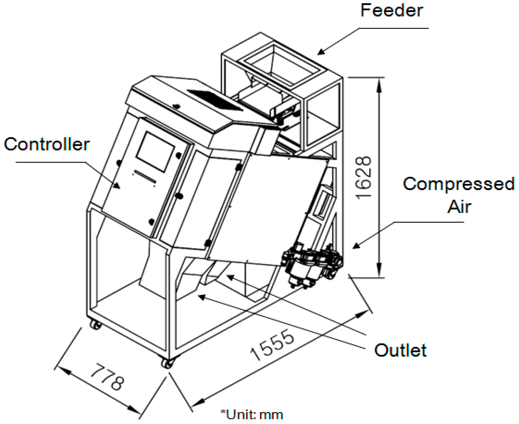
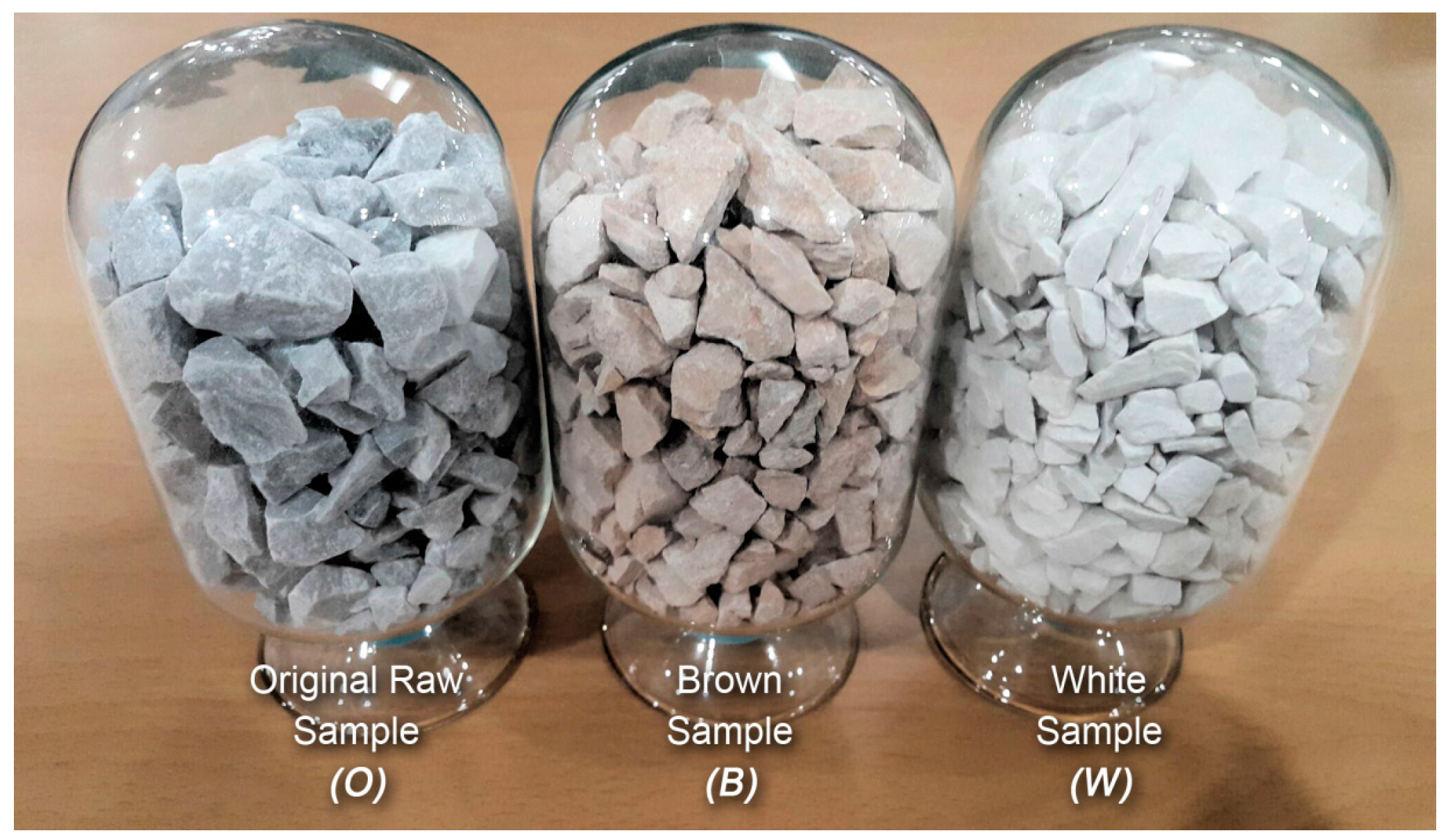
3.3. Heat Treatment and Optical Sorting

Limestone was crushed by a jaw crusher, and particles 20–35 mm in size were separated using a sieve and used in the calcination experiments. The sample was calcined using an electric furnace to induce a de-carboxylation reaction with lime (CaO). In this study, calcination was performed at 600 °C for 1 h, at a heating rate of 10 °C/min.

The optical sorting machine was designed as a suite type (rather than a belt conveyor type) machine with a short distance from the feeder to the sensing area; its schematic diagram is shown in Figure 1. The basic operating mechanism of optical sorting is that the material falling from the feeder passes through the inspection area where the optical camera is located, where the color difference is used to recognize the particles with an image processing system. Compressed air is injected to separate the rejected particles at this point.

4. Results and Discussion

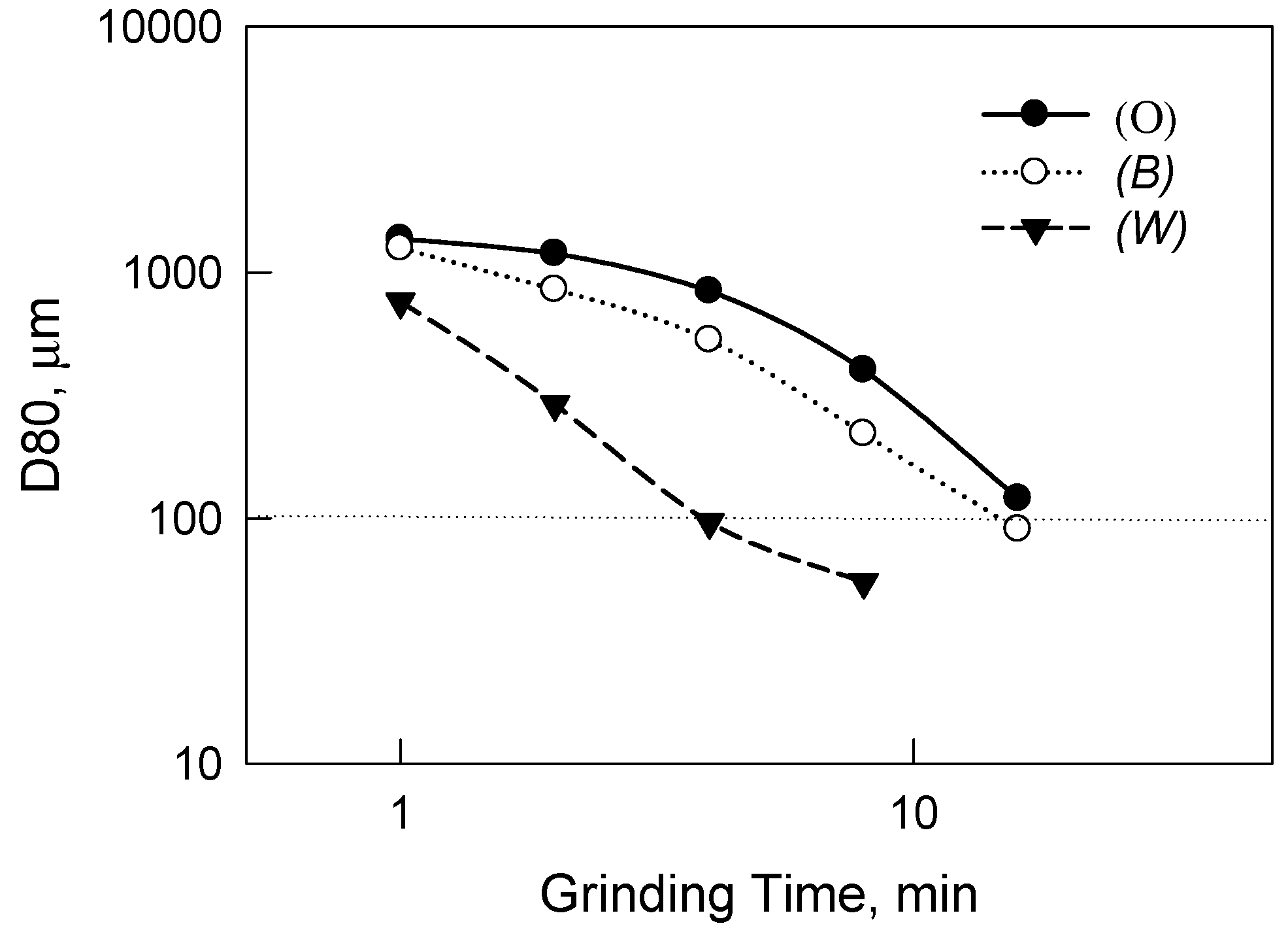
4.1. Effect of Heat Treatment on Limestone

The low-grade limestone sample was heat-treated at 600 °C in an oxidizing atmosphere. The original sample before the heat treatment process consisted of gray-scale samples of various brightness levels, but was divided into two major groups after processing: brown and white, with a very small amount of dark gray coloring (Figure 2). Figure 3 and

Table 3. XRD quantitative analysis and whiteness of heat-treated samples (B) and (W).

Sample	Calcite	Dolomite	Periclase	Muscovite	Whiteness	wt %
(B)	15	83.1	1.9	-	63.4	45
(W)	100	-	-	-	85.7	55

shows X-ray diffraction (XRD) analysis results for mineral qualitative/quantitative analyses and brightness testing for each sample. The white sample group is mostly calcite (CaCO₃) with whiteness > 86%. The brown sample group contains dolomite (CaMg(CO₃)₂), with small amount of calcite and periclase (<2%) and a whiteness < 65%. Based on the optical separation, the brown and white groups were 45% and 55% of the total mass, respectively.

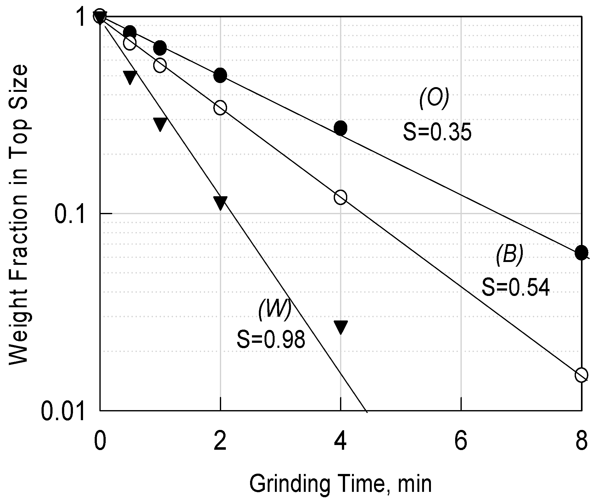
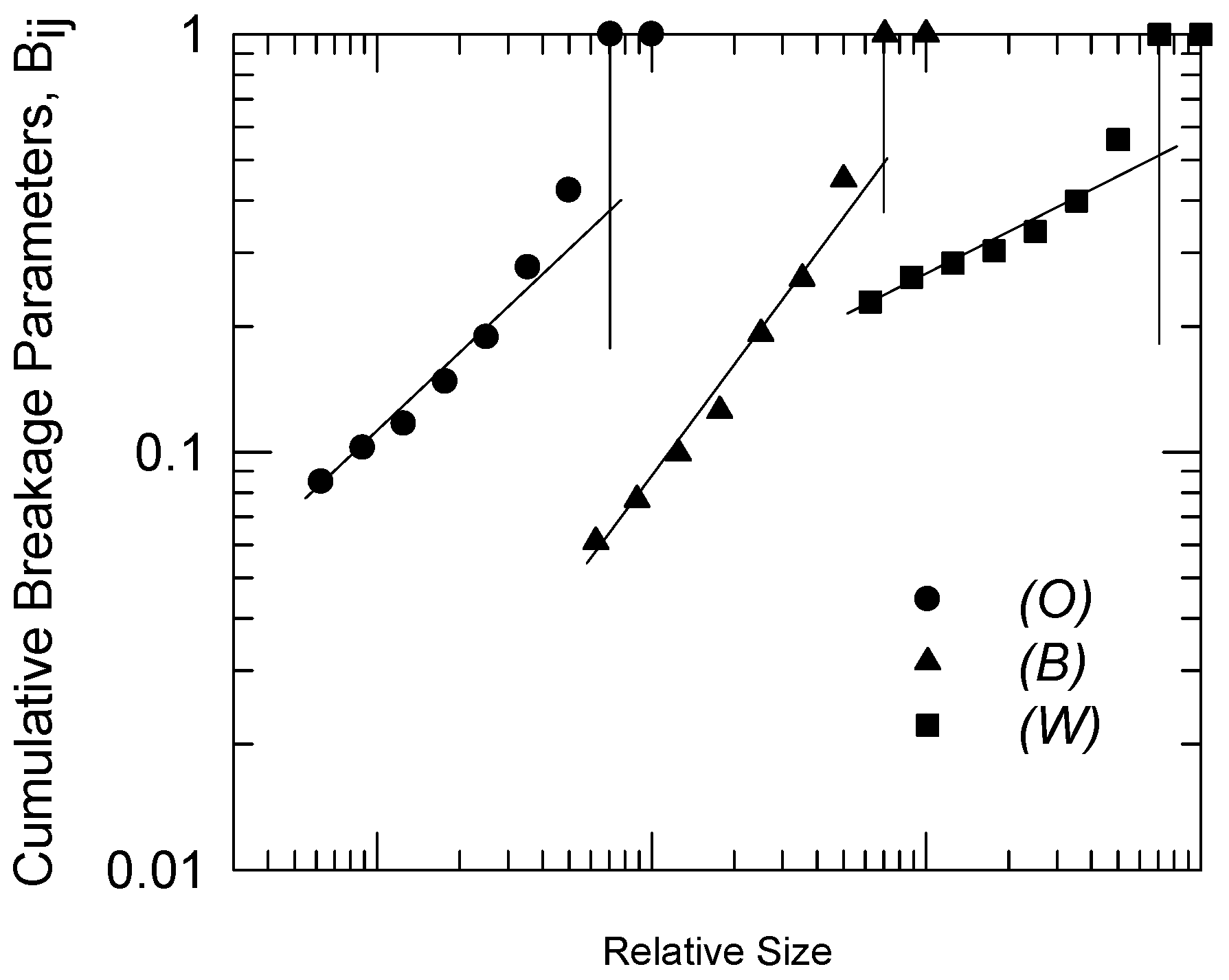
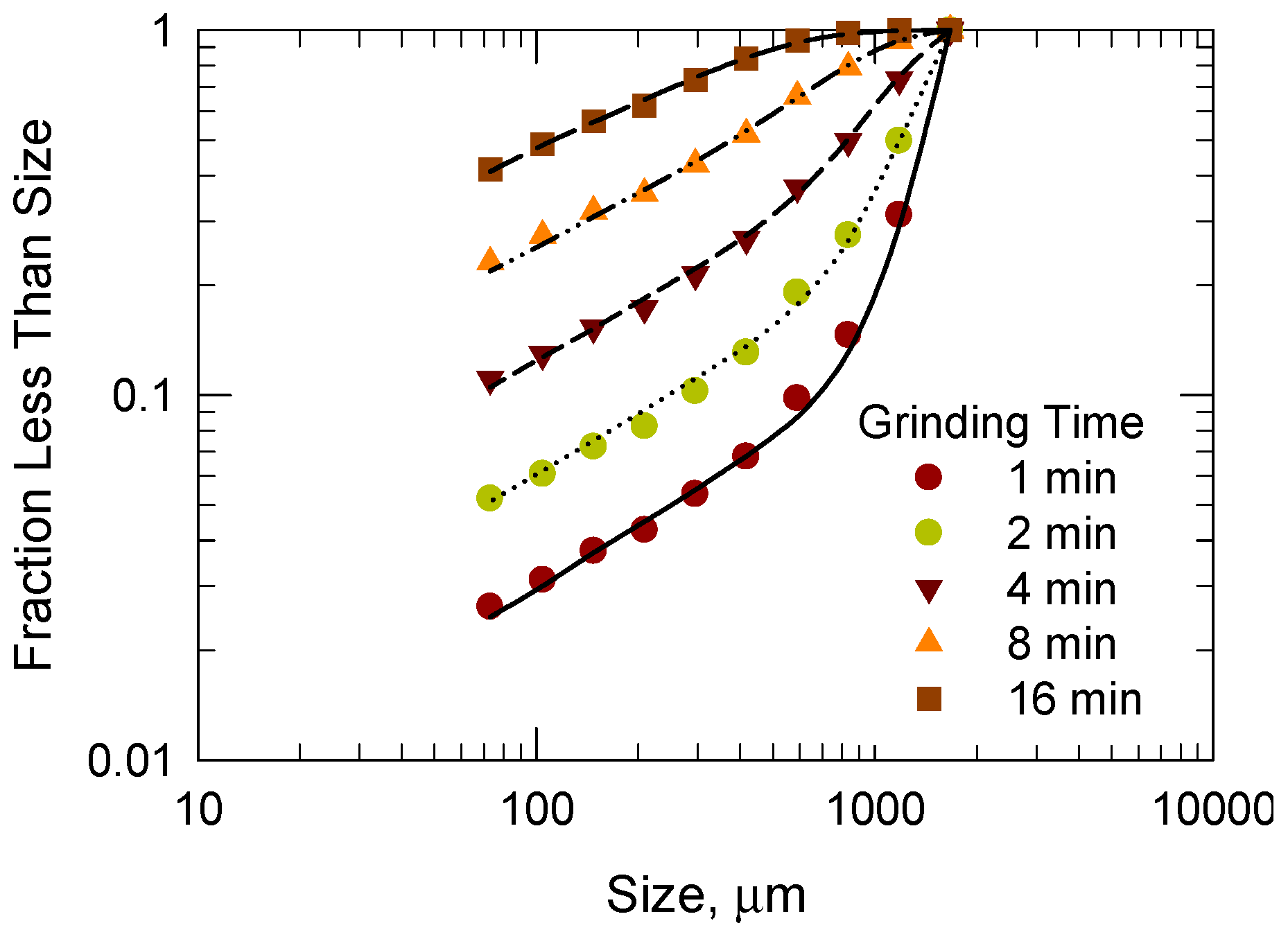
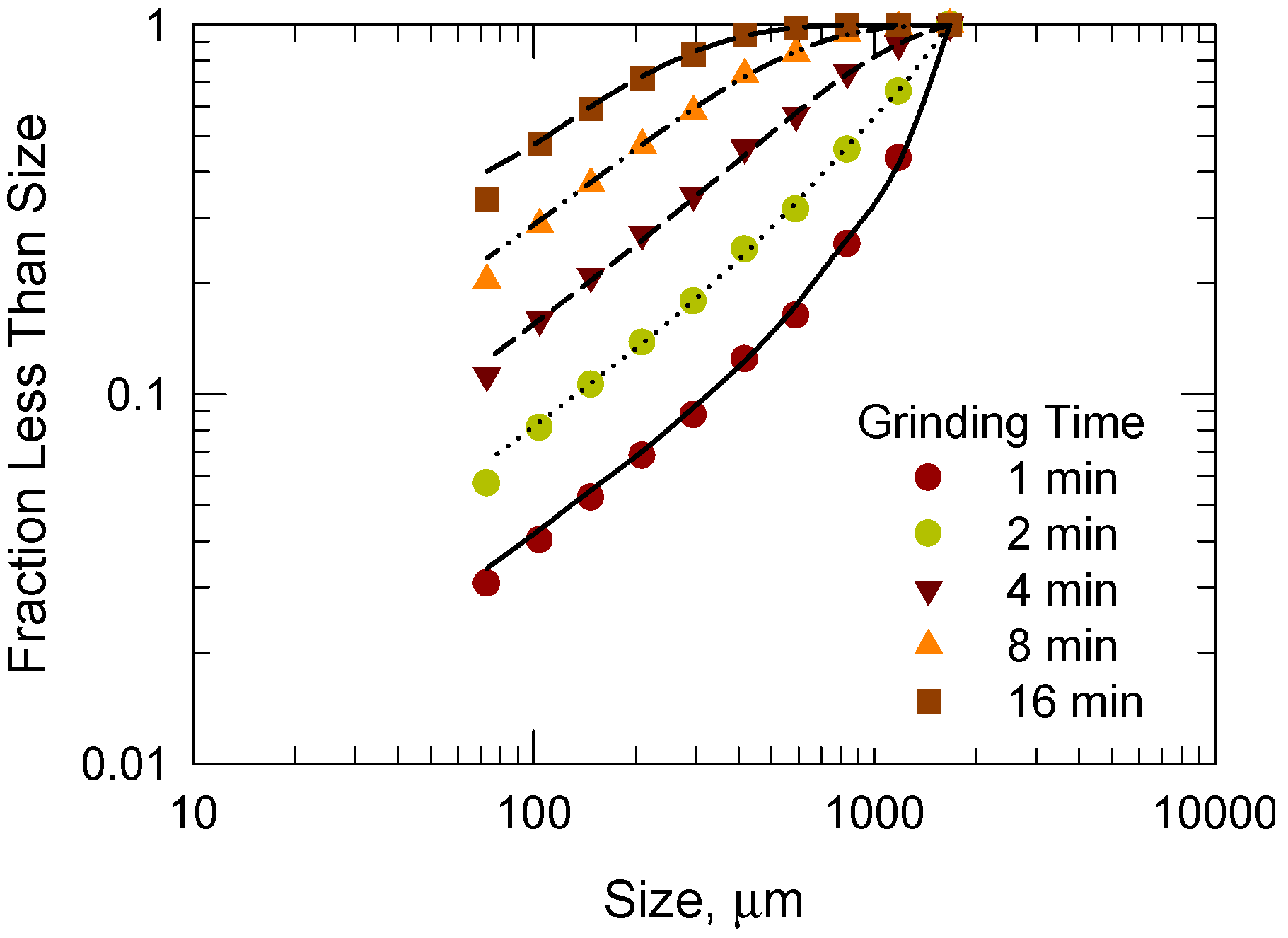
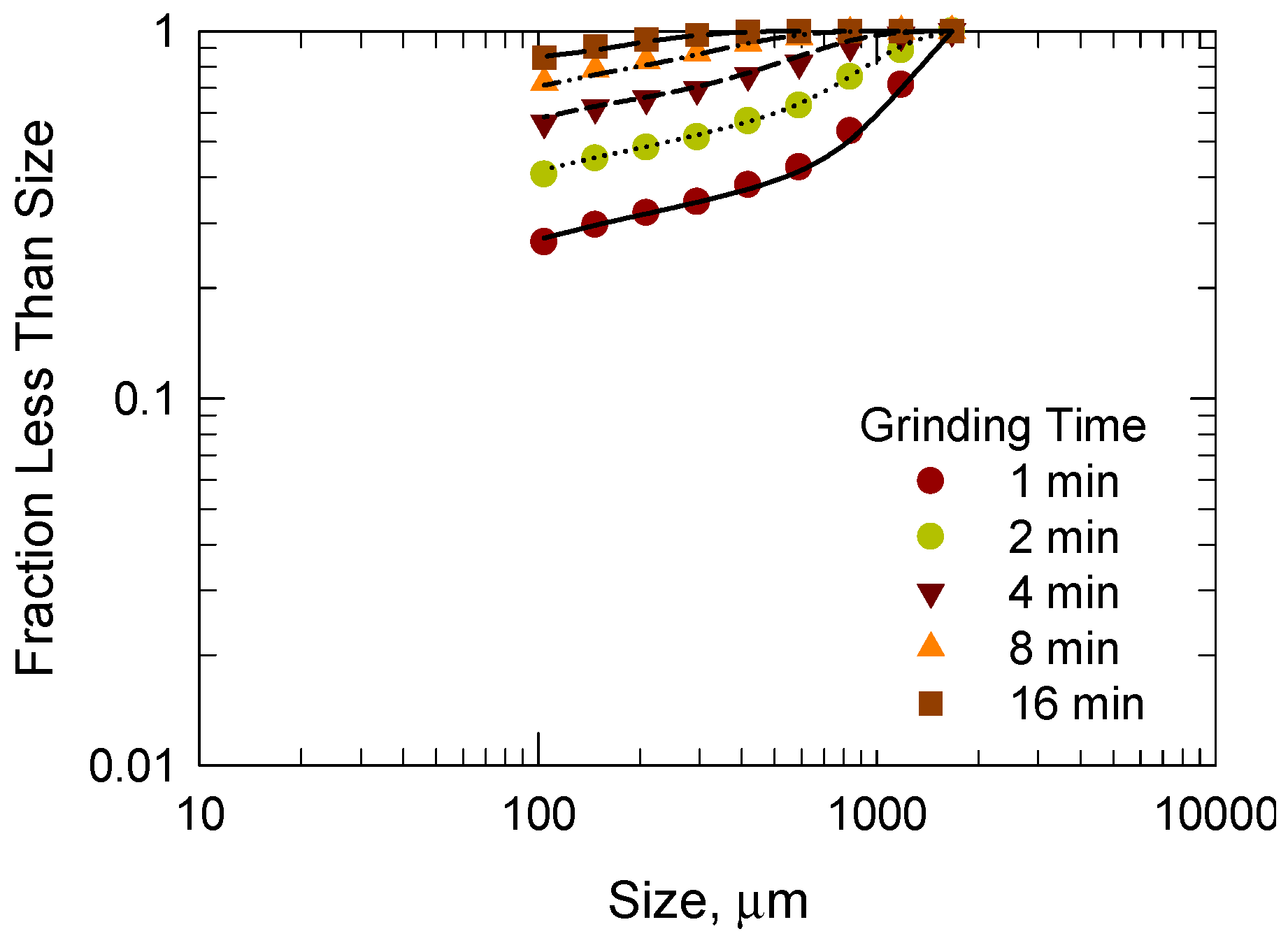
4.2. Determination of Breakage Parameters by Experimental Methods

The specific rate of breakage can be easily calculated experimentally. A sample having a single size interval was ground for a pre-determined grinding time, t. The fraction remaining in the original size interval, w(t), was measured with sieve shaker (Ro-tap). By repeating these tests several times, a graph of the weight fraction less than size against the grinding time was plotted on a semi-log scale (first-order plot), and the specific rate of breakage was determined directly from the slope.

A first-order-plot of 16 × 20 mesh samples is shown in Figure 4 to identify the specific rate of breakage S of the unheated raw limestone (hereinafter referred to as “(O)”), the brown sample group after heat treatment (“(B)”) and the white sample group after heat treatment (“(W)”). (O) and (B) show a typical linear decrease in the fraction remaining in the largest size interval, indicating ideal first-order breakage. On the other hand, (W) shows a straight decrease for up to 4 min, but afterwards more than 98% of the particles were pulverized, resulting in a large amount of fine powder, showing first-order breakage. The S values of samples (O), (B) and (W) were 0.35, 0.54 and 0.98, respectively, which means that 29%, 42%, and 56% of the largest size particles are broken down within 1 min of grinding (1 – 1/e_s).

The primary breakage distribution is usually measured experimentally using the BII method [11]: milling is performed for a small degree of grinding in which secondary breakage does not occur. Based on previous literature, the BII method gives a reasonable result: up to approximately 30% of the particles in the largest size interval are broken. Therefore, the cumulative size distribution of the ground product for 30 s of grinding time is shown in Figure 5, and the parameters calculated using the BII method are shown in

Table 4. Parameters of primary breakage distribution by BII method.

Parameters	(O)	(B)	(W)
γ	0.6	0.7	0.3
Φ	0.4	0.6	0.5
β	6.0	3.5	5.0

. In this study, 17%, 25% and 44% of the particles in the largest size interval were broken at 30 s of grinding for (O), (B) and (W), respectively. As shown in Figure 4 and Table 3, the γ values of (O) and (B), which have a large influence on the composition of the fragment after breakage, are 0.6 and 0.7, respectively. On the other hand, in the case of (W), a γ value of 0.3 means that more fine particles can be generated.

4.3. Determination of Breakage Parameters by Back-Calculation Methods

The breakage parameters can be experimentally determined, but the amount of experimental error and the difficulty in estimating the overall breakage parameters for various grinding times are relevant issues here [14]. In particular, it may be difficult to apply experimental methods when the breakage does not follow first-order kinetics. Therefore, the optimum parameters were evaluated using a back-calculation method based on nonlinear programming.

Nonlinear programming is an approach to solving optimization problems where the objective function is nonlinear. In general, the goal of nonlinear programming is to minimize any objective function within certain constraints. Equation (4) shows that there are equations and inequalities in the constraint conditions, generalized using m inequalities g_i(x) and n equations h_j(x) [12].

$$\begin{gathered} \min f\left(x\right), \\ \mathrm{sub}.\mathrm{to}{g}_i\left(x\right)\ge 0 i=1,2,\cdots ,m, \\ {h}_j\left(x\right)=0 j=1,2,\cdots ,n, \end{gathered}$$

(4)

Among the many ways to solve nonlinear programming, the simplex method, which does not use a differential, was used in this study because it is difficult to obtain the form of the differential forms of specific rate of breakage and primary breakage distribution, and the time required for the overall computation is very small. Applying the simplex method to this study, the objective function becomes the SSQ, which is the sum of squares of the difference between the experimental values and the calculated values as shown in Equation (5) [11]. The constraint is that the grinding constants are all positive, and the breakage parameters A and α are related to the specific rate of breakage, and γ, Φ, β are related to the primary breakage distribution.

$$\begin{gathered} \min {{\displaystyle \sum }}^{\text{}}{\mathrm{w}}_{\mathrm{i}}{({\mathrm{p}}_{\mathrm{i}\left(\exp .\right)}-{\mathrm{p}}_{\mathrm{i}\left(\mathrm{cal}.\right)})}^2 \\ \mathrm{sub}.\mathrm{to}A, \alpha , \gamma , \Phi , \beta >0, \end{gathered}$$

(5)

Here, w_i is the weight fraction of original material of size i and p_i is the weight fraction less than size i of the product.

Table 5. Breakage parameters obtained by back-calculation.

Breakage function	Parameters	Value
		(O)	(B)	(W)
Specific rate of breakage	A (1 mm)	0.28	0.35	0.51
	α	0.37	0.85	1.39
Primary distribution of breakage	γ	0.58	0.67	0.15
	Φ	0.36	0.41	0.50
	β	6.5	3.0	4.0

shows the results for the five breakage parameters of the three sample groups obtained using back-calculation. In this case, using the values for A and α in Equation (1), the S values of 12 mesh (1.7 mm) were 0.34, 0.54 and 1.05 for (O), (B), (W), respectively. This result is very similar to the experimental values, so it is judged that the constants calculated by the back-calculation method are reasonable. A similar tendency was observed to the values obtained by experimental methods in the case of the primary breakage distribution, but the differences between the experimental and back-calculation method increased in the order from (O) to (B) to (W). The determination of the breakage parameters by experimental methods using the BII method is inadequate because of the fast breakage in a short grinding time, as in this case.

The experimental and simulation (calculated based on parameters obtained by back-calculation) product size distributions are compared in Figure 6, Figure 7 and Figure 8 for samples (O), (B) and (W), respectively, for various grinding times. The breakage parameters determined by back-calculation were reasonably accurate when the appropriate parameters were used. The prediction values of the size distribution agree well with the actual measurements over the entire size range, and the results reflect that the back-calculated values of the two breakage functions (specific rate of breakage and primary breakage distribution) are valid.

Figure 9 shows the variation of the median particle size, d50 (50 wt % passing size) with grinding time for the three samples. As shown in the graph, compared with the original sample (O), the decrease in the median size of the samples (B) and (W) after the heat treatment was remarkable. For example, in the case of sample (W), the grinding time for reaching a median size of 100 μm was reduced from 17 min (in the case of (O)) to 4 min. Therefore, via appropriate heat treatment and optical sorting processes, the energy consumption can be greatly reduced by shortening the grinding time. By understanding the grinding characteristics of heat-treated materials based on kinetic models, the efficiency can be significantly improved, which is presently the biggest concern in the limestone industry.

5. Conclusions

Optical sorting after heat treatments of low-grade limestone and grinding tests were carried out using a ball mill. The main conclusions of this study are as follows:

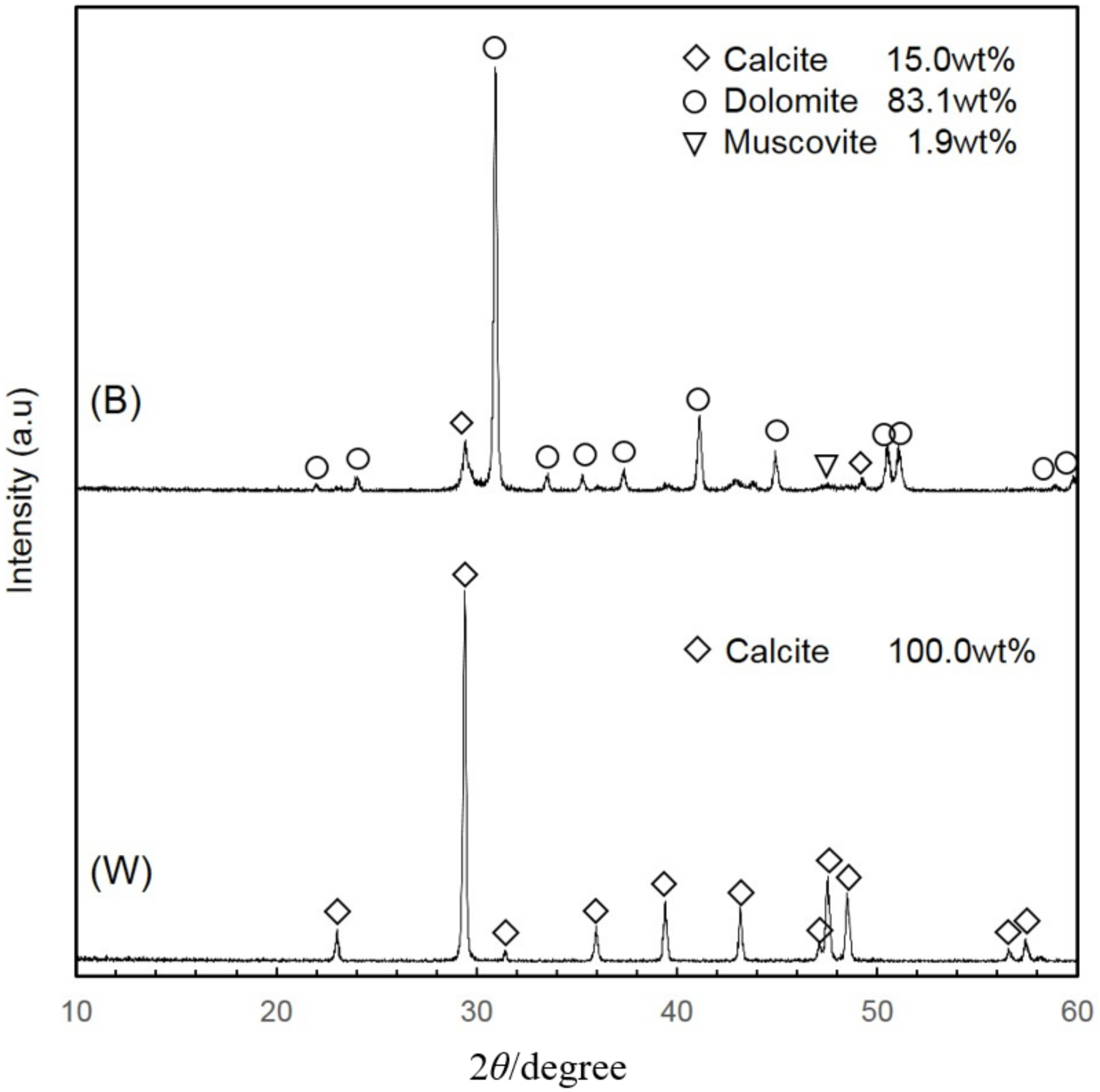
• After heat treatment at 600 °C for 1 h, low-grade limestone can be divided into brown and white groups. XRD analysis showed that the brown group consists of mainly dolomite while the white limestone is composed mainly of calcite. These were separated by the optical sorting process based on color differences, and each sample group as well as the original ore showed various grinding characteristics in the ball mill.
• The breakage parameters of the kinetic model (specific rate of breakage and primary breakage distribution) were calculated from the size distribution of the product samples, and the predicted values of the size distribution agree well with the experimental data.
• The results from this study indicate that ball mill grinding of limestone can be described based on the population-balance model. This kinetic model approach can provide a basis for the design of milling processes for the utilization of low-grade limestone. In addition, it is expected to play a major role in optimizing the grinding process and improving the efficiency of limestone production.

References

1. Cho, H.C.; Jeong, S. A characteristic study of ball mill and centrifugal mill using discrete element method. J. Miner. Energy Resour. 2005, 42, 393–402. [Google Scholar]
2. Deniz, V. A new size distribution model by t-family curves for comminution of limestones in an impact crusher. Adv. Powder Technol. 2011, 22, 761–765. [Google Scholar] [CrossRef]
3. Nitta, S.; Bissombolo, A.; Furuyama, T.; Mori, S. Relationship between bond’s work index (Wi) and uniformity constant (n) of grinding kinetics on tower mill milling limestone. Int. J. Miner. Process. 2002, 66, 79–87. [Google Scholar] [CrossRef]
4. Deniz, V. Relationships between bond’s grindability (Gbg) and breakage parameters of grinding kinetic on limestone. Powder Technol. 2004, 139, 208–213. [Google Scholar] [CrossRef]
5. Dündar, H.; Benzer, H. Investigating multicomponent breakage in cement grinding. Miner. Eng. 2015, 77, 131–136. [Google Scholar] [CrossRef]
6. Sun, H.; Hohl, B.; Cao, Y.; Handwerker, C.; Rushing, T.S.; Cummins, T.K.; Weiss, J. Jet mill grinding of portland cement, limestone, and fly ash: Impact on particle size, hydration rate, and strength. Cem. Concr. Compos. 2013, 44, 41–49. [Google Scholar] [CrossRef]
7. Guzzo, P.L.; Tino, A.A.; Santos, J.B. The onset of particle agglomeration during the dry ultrafine grinding of limestone in a planetary ball mill. Powder Technol. 2015, 284, 122–129. [Google Scholar] [CrossRef]
8. Kwade, A. Mill selection and process optimization using a physical grinding model. Int. J. Miner. Process. 2004, 74, S93–S101. [Google Scholar] [CrossRef]
9. Fuerstenau, D.; De, A.; Kapur, P. Linear and nonlinear particle breakage processes in comminution systems. Int. J. Miner. Process. 2004, 74, S317–S327. [Google Scholar] [CrossRef]
10. Lai, H.-Y. A high-precision surface grinding model for general ball-end milling cutters. Int. J. Adv. Manuf. Technol. 2002, 19, 393–402. [Google Scholar] [CrossRef]
11. Austin, L.G.; Klimpel, R.R.; Luckie, P.T. Process Engineering of Size Reduction: Ball Milling; American Institute of Mining, Metallurgical, and Petroleum Engineers: New York, NY, USA, 1984. [Google Scholar]
12. Avriel, M. Nonlinear Programming: Analysis and Methods; Courier Corporation: North Chelmsford, MA, USA, 2003. [Google Scholar]
13. Lee, H.; Kim, H.K.; Kim, W.T.; Kim, S.B. Determination of breakage parameters in mathematical grinding model by weight-adjustment modification. J. Miner. Energy Resour. 2013, 50, 80–87. [Google Scholar] [CrossRef]
14. Lee, H.; Cho, H.C.; Kwon, J.H. Using the discrete element method to analyze the breakage rate in a centrifugal/vibration mill. Powder Technol. 2010, 198, 364–372. [Google Scholar] [CrossRef]
Figure 1. Schematic diagram of the optical sorter in this study.
Minerals 08 00018 g001
Figure 2. Three types of sample material groups; original raw sample (O), brown sample (B) and white sample (W).
Minerals 08 00018 g002
Figure 3. XRD results of heat-treated samples (B) and (W).
Minerals 08 00018 g003
Figure 4. First-order-plot for the 16 × 20 mesh materials (O), (B) and (W).
Minerals 08 00018 g004
Figure 5. Cumulative breakage distribution for the 16 × 20 mesh materials (O), (B) and (W).
Minerals 08 00018 g005
Figure 6. Experimental and simulation product size distributions for various batch grinding times (solid lines indicate the simulation results) for (O).
Minerals 08 00018 g006
Figure 7. Experimental and simulation product size distributions for various batch grinding times (solid lines indicate the simulation results) for (B).
Minerals 08 00018 g007
Figure 8. Experimental and simulation product size distributions for various batch grinding times (solid lines indicate the simulation results) for (W).
Minerals 08 00018 g008
Figure 9. Median size (50% passing size) for various batch grinding times.
Minerals 08 00018 g009