
Fast Initial Model Design for Electrical Resistivity Inversion by Using Broad Learning Framework
 , , ,
, , ,
Abstract
:1. Introduction
2. Materials and Methods
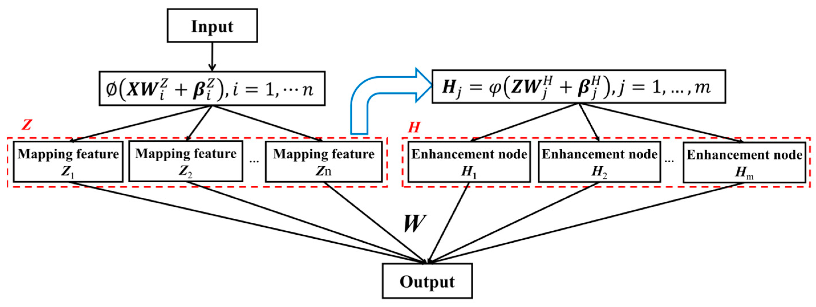
2.1. BL Framework for Initial Resistivity Model Design
2.2. Generation of Training Dataset
2.3. Select of Training Dataset Size
2.4. Choose of BL Network Complexity
2.5. L-BFGS Inversion with Designed Initial Model
- Set fitting tolerance error and a maximum number of iterations Num. Input apparent resistivity data and the designed initial resistivity model ;
- Calculate the apparent resistivity data of the current th iteration resistivity model by forward modeling: ;
- Calculate the partial derivative of Equation (6), and calculate the search direction . Obtain the appropriate step by line search and update resistivity model ;
- Compute the misfit between observed data and calculated data . If or inversion stop; otherwise, set and go to step 2.
3. Results
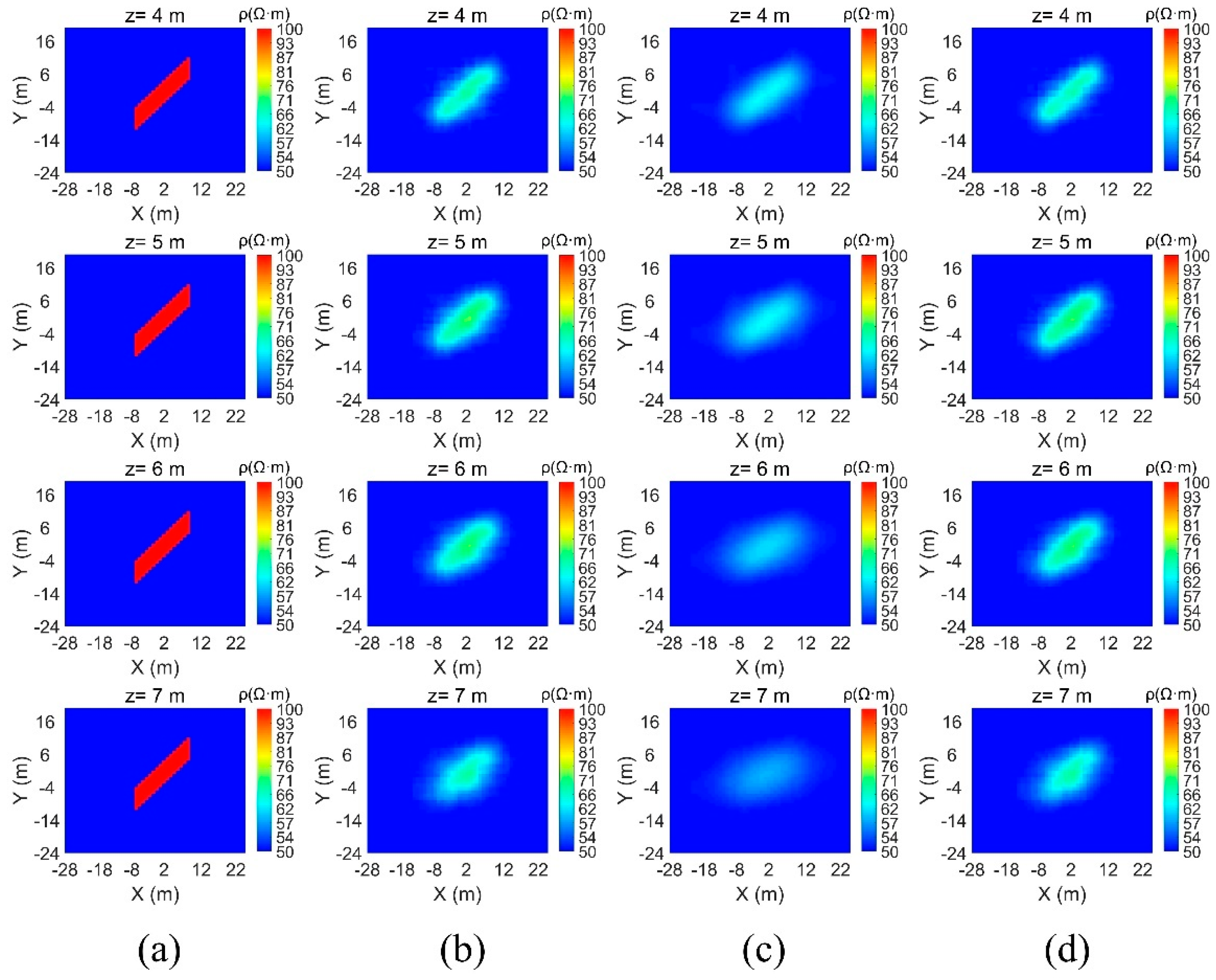
3.1. Synthetic Experiment 1
3.2. Synthetic Experiment 2
3.3. Synthetic Experiment 3
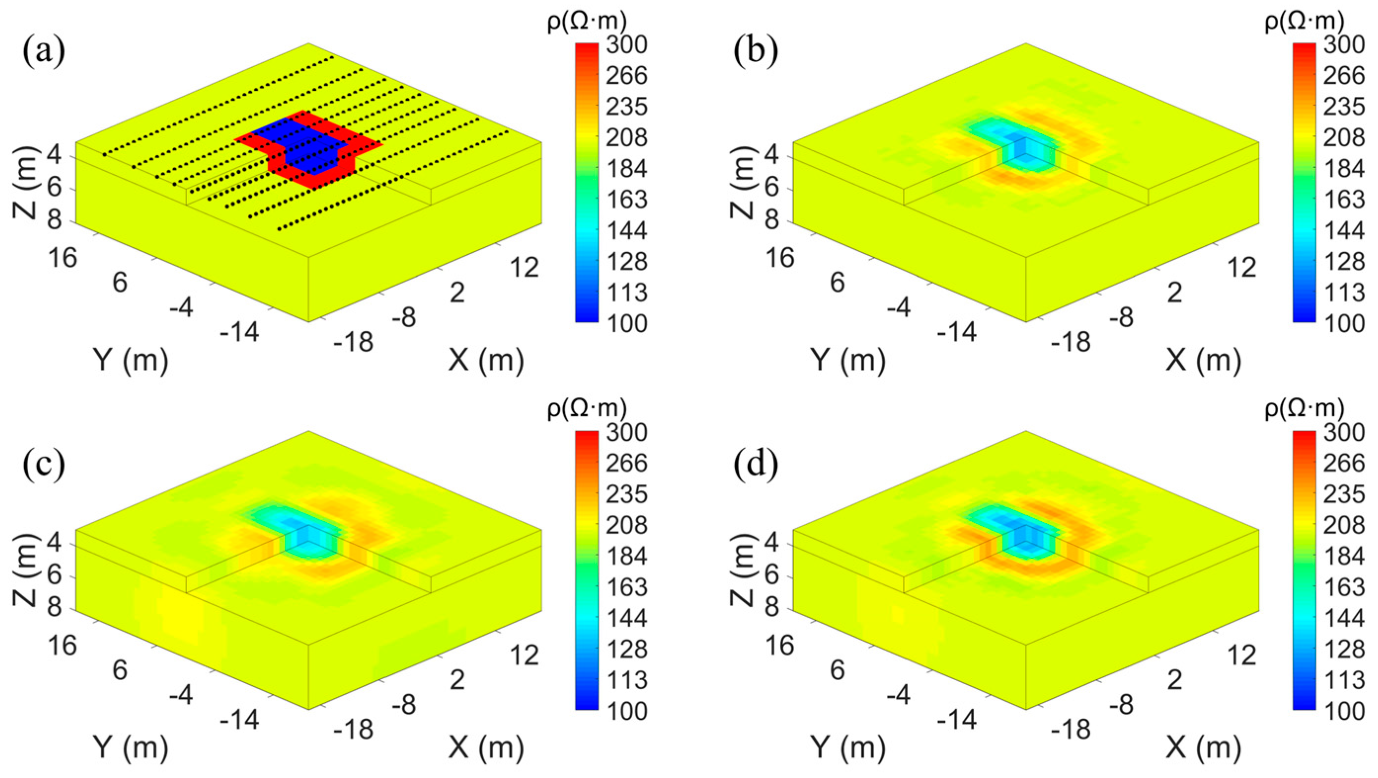
3.4. Synthetic Experiment 4
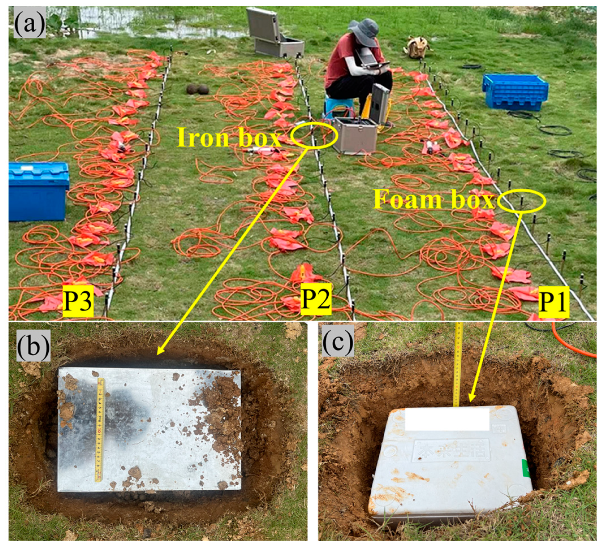
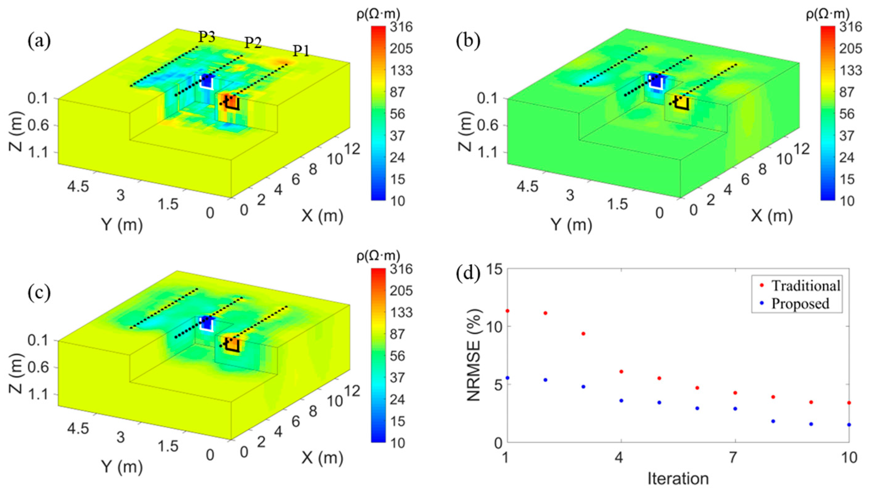
3.5. Field Experiment
4. Discussion
4.1. Generalization Ability of BL Network
4.2. Noise Resistance Test
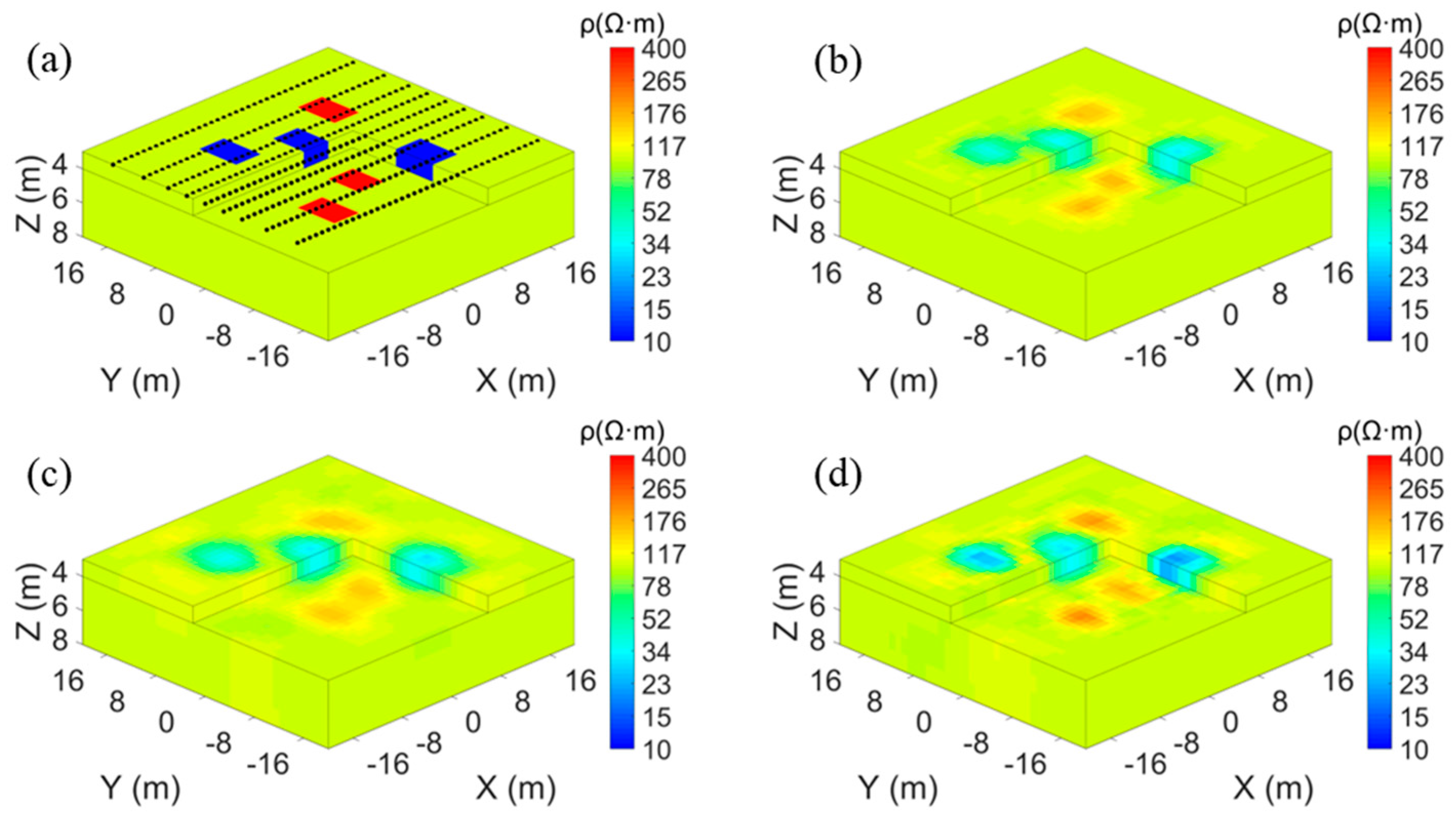
4.3. Checkerboard Test
5. Conclusions
Author Contributions
Funding
Data Availability Statement
Acknowledgments
Conflicts of Interest
References
- Cardarelli, E.; Cercato, M.; Di Filippo, G. Geophysical investigation for the rehabilitation of a flood control embankment. Near Surf. Geophys. 2010, 8, 287–296. [Google Scholar] [CrossRef]
- Ibraheem, I.M.; Tezkan, B.; Bergers, R. Integrated interpretation of magnetic and ERT data to characterize a landfill in the north-west of Cologne, Germany. Pure Appl. Geophys. 2021, 178, 2127–2148. [Google Scholar] [CrossRef]
- Yu, N.; Liu, H.; Feng, X.; Li, T.; Du, B.; Wang, C.; Wang, W.; Kong, W. Advancing CO2 Storage Monitoring via Cross-Borehole Apparent Resistivity Imaging Simulation. IEEE Trans. Geosci. Remote Sens. 2023, 61, 1–12. [Google Scholar] [CrossRef]
- Ali, M.A.H.; Mewafy, F.M.; Qian, W.; Alshehri, F.; Ahmed, M.S.; Saleem, H.A. Integration of Electrical Resistivity Tomography and Induced Polarization for Characterization and Mapping of (Pb-Zn-Ag) Sulfide Deposits. Minerals 2023, 13, 986. [Google Scholar] [CrossRef]
- Uhlemann, S.; Chambers, J.; Falck, W.E.; Tirado Alonso, A.; Fernández González, J.L.; de Gea, A.E. Applying electrical resistivity tomography in ornamental stone mining: Challenges and solutions. Minerals 2018, 8, 491. [Google Scholar] [CrossRef]
- Shin, Y.; Shin, S.; Cho, S.-J.; Son, J.-S. Application of 3D Electrical Resistivity Tomography in the Yeoncheon Titanomagnetite Deposit, South Korea. Minerals 2021, 11, 563. [Google Scholar] [CrossRef]
- Su, Z.; Revil, A.; Ghorbani, A.; Zhang, X.; Zhao, X.; Richard, J. Combining Electrical Resistivity, Induced Polarization, and Self-Potential for a Better Detection of Ore Bodies. Minerals 2023, 14, 12. [Google Scholar] [CrossRef]
- Vu, M.; Jardani, A. Convolutional neural networks with SegNet architecture applied to three-dimensional tomography of subsurface electrical resistivity: CNN-3D-ERT. Geophys. J. Int. 2021, 225, 1319–1331. [Google Scholar] [CrossRef]
- Sharma, S.P. VFSARES—A very fast simulated annealing FORTRAN program for interpretation of 1-D DC resistivity sounding data from various electrode arrays. Comput. Geosci. 2012, 42, 177–188. [Google Scholar] [CrossRef]
- Başokur, A.T.; Akca, I. Object-based model verification by a genetic algorithm approach: Application in archeological targets. J. Appl. Geophys. 2011, 74, 167–174. [Google Scholar] [CrossRef]
- Liu, B.; Li, S.; Nie, L.; Wang, J.; Zhang, Q. 3D resistivity inversion using an improved Genetic Algorithm based on control method of mutation direction. J. Appl. Geophys. 2012, 87, 1–8. [Google Scholar] [CrossRef]
- Barboza, F.M.; Medeiros, W.E.; Santana, J.M. A user-driven feedback approach for 2D direct current resistivity inversion based on particle swarm optimization Feedback inversion using PSO. Geophysics 2019, 84, E105–E124. [Google Scholar] [CrossRef]
- Sosa, A.; Velasco, A.A.; Velazquez, L.; Argaez, M.; Romero, R. Constrained optimization framework for joint inversion of geophysical data sets. Geophys. J. Int. 2013, 195, 1745–1762. [Google Scholar] [CrossRef]
- Aleardi, M.; Vinciguerra, A.; Hojat, A. A convolutional neural network approach to electrical resistivity tomography. J. Appl. Geophys. 2021, 193, 104434. [Google Scholar] [CrossRef]
- Alyousuf, T.; Li, Y. Inversion using adaptive physics-based neural network: Application to magnetotelluric inversion. Geophys. Prospect. 2022, 70, 1252–1272. [Google Scholar] [CrossRef]
- Pidlisecky, A.; Haber, E.; Knight, R. RESINVM3D: A 3D resistivity inversion package. Geophysics 2007, 72, H1–H10. [Google Scholar] [CrossRef]
- Wu, P.; Tan, H.; Tao, T.; Ma, H.; Ding, Z.; Xu, L. Three-dimensional joint inversion of the resistivity method and ambient noise method with cross-gradient constraints. Chin. J. Geophys. 2020, 63, 3912–3930. [Google Scholar]
- Wu, X.; Xu, G. Study on 3-D resistivity inversion using conjugate gradient method. Chin. J. Geophys. 2000, 43, 450–458. [Google Scholar]
- Peng, M.; Tan, H.; Moorkamp, M. Structure-coupled 3-D imaging of magnetotelluric and wide-angle seismic reflection/refraction data with interfaces. J. Geophys. Res. Solid Earth 2019, 124, 10309–10330. [Google Scholar] [CrossRef]
- Kong, W.; Tan, H.; Lin, C.; Unsworth, M.; Lee, B.; Peng, M.; Wang, M.; Tong, T. Three-Dimensional Inversion of Magnetotelluric Data for a Resistivity Model with Arbitrary Anisotropy. J. Geophys. Res. Solid Earth 2021, 126, e2020JB020562. [Google Scholar] [CrossRef]
- Xu, L.; Tan, H.; Wu, P.; Peng, M.; Wang, S.; Jiang, M. Electrical characteristics of the crust in the south part of Longmenshan fault zone: Evidence from magnetotelluric inversion with velocity structure constraints. Chin. J. Geophys. 2022, 65, 3434–3450. [Google Scholar]
- Ma, H.; Guo, Y.; Wu, P.; Tan, H. 3-D joint inversion of multi-array data set in the resistivity method based on MPI parallel algorithm. Chin. J. Geophys. 2018, 61, 5052–5065. [Google Scholar]
- Wilson, B.; Singh, A.; Sethi, A. Appraisal of Resistivity Inversion Models with Convolutional Variational Encoder–Decoder Network. IEEE Trans. Geosci. Remote Sens. 2022, 60, 1–10. [Google Scholar] [CrossRef]
- Yuval, D.; Oldenburg, W. DC resistivity and IP methods in acid mine drainage problems: Results from the Copper Cliff mine tailings impoundments. J. Appl. Geophys. 1996, 34, 187–198. [Google Scholar] [CrossRef]
- Wunderlich, T.; Fischer, P.; Wilken, D.; Hadler, H.; Erkul, E.; Mecking, R.; Günther, T.; Heinzelmann, M.; Vött, A.; Rabbel, W. Constraining electric resistivity tomography by direct push electric conductivity logs and vibracores: An exemplary study of the Fiume Morto silted riverbed (Ostia Antica, western Italy). Geophysics 2018, 83, B87–B103. [Google Scholar] [CrossRef]
- Pidlisecky, A.; Knight, R.; Haber, E. Cone-based electrical resistivity tomography. Geophysics 2006, 71, G157–G167. [Google Scholar] [CrossRef]
- Loke, M.H.; Barker, R.D. Rapid least-squares inversion of apparent resistivity pseudosections by a quasi-Newton method1. Geophys. Prospect. 1996, 44, 131–152. [Google Scholar] [CrossRef]
- Günther, T.; Rücker, C.; Spitzer, K. Three-dimensional modelling and inversion of DC resistivity data incorporating topography—II. Inversion. Geophys. J. Int. 2006, 166, 506–517. [Google Scholar] [CrossRef]
- Wagner, F.; Mollaret, C.; Günther, T.; Kemna, A.; Hauck, C. Quantitative imaging of water, ice and air in permafrost systems through petrophysical joint inversion of seismic refraction and electrical resistivity data. Geophys. J. Int. 2019, 219, 1866–1875. [Google Scholar] [CrossRef]
- Palacios, A.; Ledo, J.J.; Linde, N.; Luquot, L.; Bellmunt, F.; Folch, A.; Marcuello, A.; Queralt, P.; Pezard, P.A.; Martínez, L. Time-lapse cross-hole electrical resistivity tomography (CHERT) for monitoring seawater intrusion dynamics in a Mediterranean aquifer. Hydrol. Earth Syst. Sci. 2020, 24, 2121–2139. [Google Scholar] [CrossRef]
- Goebel, M.; Knight, R.; Kang, S. Enhancing the resolving ability of electrical resistivity tomography for imaging saltwater intrusion through improvements in inversion methods: A laboratory and numerical study. Geophysics 2021, 86, WB101–WB115. [Google Scholar] [CrossRef]
- Slezak, K.; Jozwiak, W.; Nowozynski, K.; Orynski, S.; Brasse, H. 3-D studies of MT data in the Central Polish Basin: Influence of inversion parameters, model space and transfer function selection. J. Appl. Geophys. 2019, 161, 26–36. [Google Scholar] [CrossRef]
- Mousavi, S.M.; Beroza, G.C. Deep-learning seismology. Science 2022, 377, eabm4470. [Google Scholar] [CrossRef] [PubMed]
- Qi, J.; Zhang, J.; Lyu, B.; Marfurt, K.J. Seismic Geometric Nonparallelism Attributes. IEEE Geosci. Remote Sens. Lett. 2020, 19, 1–5. [Google Scholar] [CrossRef]
- Wu, S.; Huang, Q.; Zhao, L. De-noising of transient electromagnetic data based on the long short-term memory-autoencoder. Geophys. J. Int. 2021, 224, 669–681. [Google Scholar] [CrossRef]
- Xue, J.; Huang, Q.; Wu, S.; Nagao, T. LSTM-Autoencoder Network for the Detection of Seismic Electric Signals. IEEE Trans. Geosci. Remote Sens. 2022, 60, 1–12. [Google Scholar] [CrossRef]
- Wu, S.; Huang, Q.; Zhao, L. Convolutional neural network inversion of airborne transient electromagnetic data. Geophys. Prospect. 2021, 69, 1761–1772. [Google Scholar] [CrossRef]
- Wu, S.; Huang, Q.; Zhao, L. Instantaneous inversion of airborne electromagnetic data based on deep learning. Geophys. Res. Lett. 2022, 49, e2021GL097165. [Google Scholar] [CrossRef]
- Wu, S.; Huang, Q.; Zhao, L. Fast Bayesian Inversion of Airborne Electromagnetic Data Based on the Invertible Neural Network. IEEE Trans. Geosci. Remote Sens. 2023, 61, 1–11. [Google Scholar] [CrossRef]
- Zhang, C.; Li, J.; Yu, H.; Liu, B. Autoencoded Elastic Wave-Equation Traveltime Inversion: Toward Reliable Near-Surface Tomogram. IEEE Trans. Geosci. Remote Sens. 2023, 61, 1–13. [Google Scholar] [CrossRef]
- Liu, B.; Guo, Q.; Li, S.; Liu, B.; Ren, Y.; Pang, Y.; Guo, X.; Liu, L.; Jiang, P. Deep learning inversion of electrical resistivity data. IEEE Trans. Geosci. Remote Sens. 2020, 58, 5715–5728. [Google Scholar] [CrossRef]
- Liu, B.; Pang, Y.; Jiang, P.; Liu, Z.; Liu, B.; Zhang, Y.; Cai, Y.; Liu, J. Physics-Driven Deep Learning Inversion for Direct Current Resistivity Survey Data. IEEE Trans. Geosci. Remote Sens. 2023, 61, 1–11. [Google Scholar] [CrossRef]
- Li, Y.; Yang, D. Electrical imaging of hydraulic fracturing fluid using steel-cased wells and a deep-learning method Electrical hydraulic fracturing imaging. Geophysics 2021, 86, E315–E332. [Google Scholar] [CrossRef]
- Chen, C.P.; Liu, Z. Broad learning system: An effective and efficient incremental learning system without the need for deep architecture. IEEE Trans. Neural Netw. Learn. Syst. 2017, 29, 10–24. [Google Scholar] [CrossRef]
- Kong, S.; Oh, J.; Yoon, D.; Ryu, D.-W.; Kwon, H.-S. Integrating Deep Learning and Deterministic Inversion for Enhancing Fault Detection in Electrical Resistivity Surveys. Appl. Sci. 2023, 13, 6250. [Google Scholar] [CrossRef]
- Yang, X.-H.; Han, P.; Yang, Z.; Miao, M.; Sun, Y.-C.; Chen, X. Broad Learning Framework for Search Space Design in Rayleigh Wave Inversion. IEEE Trans. Geosci. Remote Sens. 2022, 60, 1–17. [Google Scholar] [CrossRef]
- Yang, X.-H.; Han, P.; Yang, Z.; Chen, X. Two-stage broad learning inversion framework for shear-wave velocity estimation. Geophysics 2023, 88, WA219–WA237. [Google Scholar] [CrossRef]
- Hu, K.; Ren, H.; Huang, Q.; Zeng, L.; Butler, K.E.; Jougnot, D.; Linde, N.; Holliger, K. Water Table and Permeability Estimation from Multi-Channel Seismoelectric Spectral Ratios. J. Geophys. Res. Solid Earth 2023, 128, e2022JB025505. [Google Scholar] [CrossRef]
- Zhou, Y.; Li, X.; Tang, Q.; Kuok, S.C.; Fei, K.; Gao, L. An Assimilating Model Using Broad Learning System for Incorporating Multi-Source Precipitation Data with Environmental Factors Over Southeast China. Earth Space Sci. 2022, 9, e2021EA002043. [Google Scholar] [CrossRef]
- Byrd, R.H.; Lu, P.; Nocedal, J.; Zhu, C. A limited memory algorithm for bound constrained optimization. SIAM J. Sci. Comput. 1995, 16, 1190–1208. [Google Scholar] [CrossRef]
- Colombo, D.; Turkoglu, E.; Li, W.; Sandoval-Curiel, E.; Rovetta, D. Physics-driven deep-learning inversion with application to transient electromagnetics. Geophysics 2021, 86, E209–E224. [Google Scholar] [CrossRef]
- Nocedal, J. Updating quasi-Newton matrices with limited storage. Math. Comput. 1980, 35, 773–782. [Google Scholar] [CrossRef]
- Wang, T.; Wang, K.-P.; Tan, H.-D. Forward modeling and inversion of tensor CSAMT in 3D anisotropic media. Appl. Geophys. 2017, 14, 590–605. [Google Scholar] [CrossRef]


| Number of Training Dataset | 6000 | 8000 | 10,000 | 11,000 | 12,000 |
|---|---|---|---|---|---|
| MAPE of the training dataset (%) | 1.26 | 1.16 | 1.07 | 1.02 | 0.99 |
| MAPE of the validation dataset (%) | 1.06 | 1.04 | 1.03 | 1.02 | 1.02 |
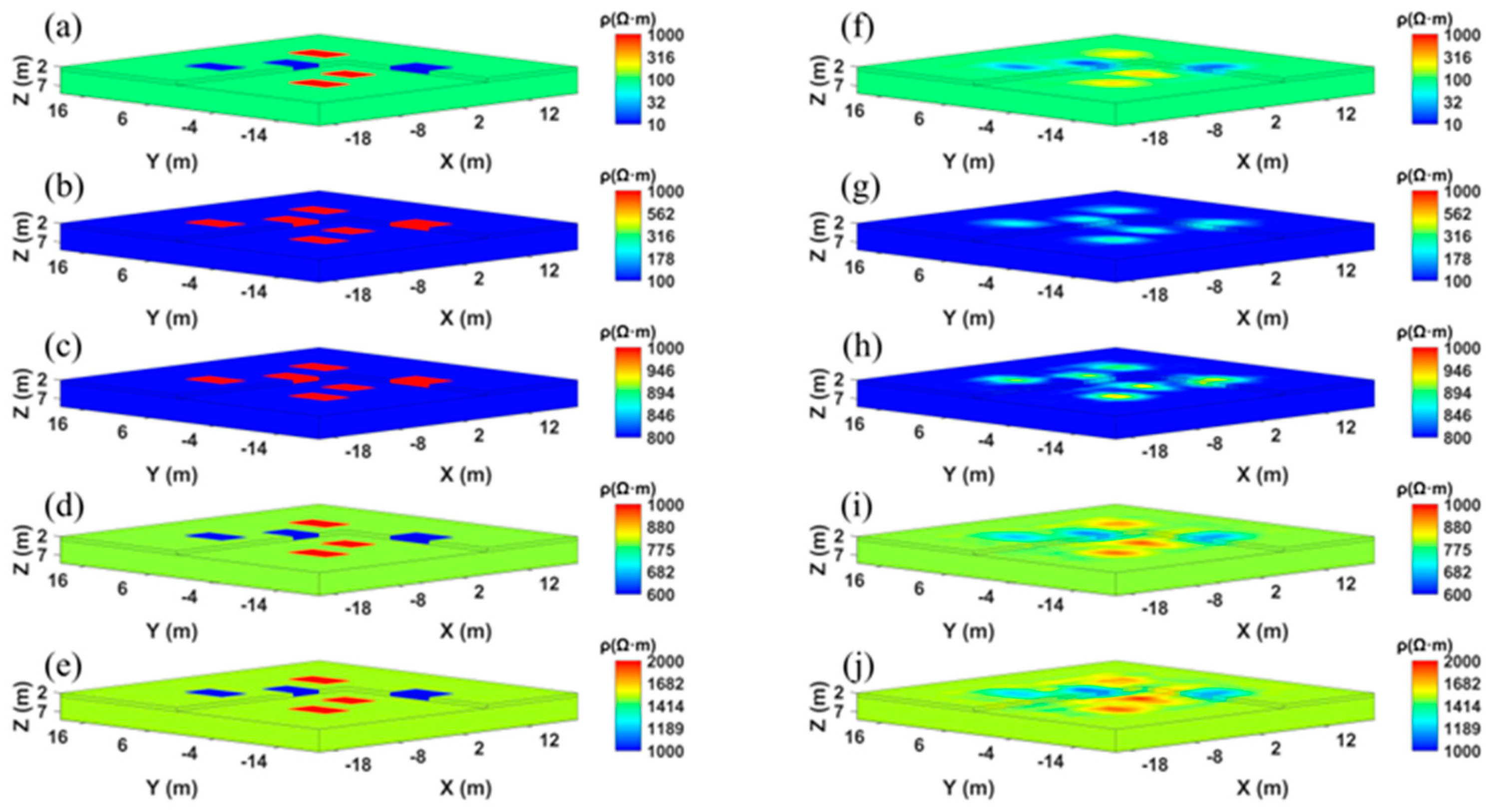
| Synthetic Model | Low Resistivity | High Resistivity | Background Resistivity | MAPE (%) |
|---|---|---|---|---|
| (a) | 10 Ω·m | 1000 Ω·m | 100 Ω·m | 4.34 |
| (b) | 1000 Ω·m | 100 Ω·m | 3.12 | |
| (c) | 1000 Ω·m | 800 Ω·m | 0.43 | |
| (d) | 600 Ω·m | 1000 Ω·m | 800 Ω·m | 0.51 |
| (e) | 1000 Ω·m | 2000 Ω·m | 1500 Ω·m | 0.98 |
Disclaimer/Publisher’s Note: The statements, opinions and data contained in all publications are solely those of the individual author(s) and contributor(s) and not of MDPI and/or the editor(s). MDPI and/or the editor(s) disclaim responsibility for any injury to people or property resulting from any ideas, methods, instructions or products referred to in the content. |
© 2024 by the authors. Licensee MDPI, Basel, Switzerland. This article is an open access article distributed under the terms and conditions of the Creative Commons Attribution (CC BY) license (https://creativecommons.org/licenses/by/4.0/).
Share and Cite
Tao, T.; Han, P.; Yang, X.-H.; Zu, Q.; Hu, K.; Mo, S.; Li, S.; Luo, Q.; He, Z. Fast Initial Model Design for Electrical Resistivity Inversion by Using Broad Learning Framework. Minerals 2024, 14, 184. https://doi.org/10.3390/min14020184
Tao T, Han P, Yang X-H, Zu Q, Hu K, Mo S, Li S, Luo Q, He Z. Fast Initial Model Design for Electrical Resistivity Inversion by Using Broad Learning Framework. Minerals. 2024; 14(2):184. https://doi.org/10.3390/min14020184
Chicago/Turabian StyleTao, Tao, Peng Han, Xiao-Hui Yang, Qiang Zu, Kaiyan Hu, Shuangling Mo, Shuangshuang Li, Qiang Luo, and Zhanxiang He. 2024. "Fast Initial Model Design for Electrical Resistivity Inversion by Using Broad Learning Framework" Minerals 14, no. 2: 184. https://doi.org/10.3390/min14020184