Unlocking the Secondary Critical Raw Material Potential of Historical Mine Sites, Lousal Mine, Southern Portugal

Abstract

A steady supply of mineral raw materials is vital for the transition to a low-carbon, circular economy. The number of active mines in Europe has severely declined over the last century and half, giving rise to many abandoned mining waste sites and corresponding geological heritage. Also, the rise in minerals demand for large-scale deployment of renewable energy requires the continued and steady availability of key minerals. The supply risk associated with unpredicted geopolitical events needs to be eliminated/mitigated. Historical mine waste sites are the answer but evaluating mine waste is a lengthy and costly exercise. The study, undertaken in the Lousal Mine, used small unmanned aerial systems (sUASs) to model and determine mine waste volumes by generating orthomosaic maps with quick, inexpensive, and reliable results. Calculated mine waste volumes between 308,478 m³ and 322,455 m³ were obtained. XRD and p-XRF techniques determined the mineralogy and chemistry of waste, which varied from mineralization and host rocks with hydrothermal alteration and numerous neogenic sulphates (mostly gypsum, rhomboclase, ferricopiapite, coquimbite, and jarosite) related with supergene processes and weathering. The study shows the viability of using these sUASs to successfully model historical mine waste sites in an initial phase and for future monitoring programs.

1. Introduction

Critical and strategic raw materials are vital for economic and technological development, key to innovation and growth in high-tech industries and critical for the transition to a low-carbon circular, rather than linear, economy, in Europe [1,2].

Active mines in Europe have declined from around 65% to approximately 5% in the last century and a half [3,4].

Hund et al. [5] has confirmed the overall rise in mineral demand. Meeting the challenge of the large-scale deployment of renewable energy requires the continued and steady availability of a variety of key minerals as well as stable prices and minimal market disruptions, which means that minerals must be imported to meet European value chain demands.

Therefore, while the EU is self-sufficient in construction minerals, in particular aggregates, and the second largest producer of certain industrial minerals, the EU remains highly dependent on imports of metallic minerals [1,2,3,6], even though there is a significant accumulated geological knowledge and detailed mapping, stratigraphy and metallogeny of the European mineral provinces.

While importing the necessary raw materials seems to be an “easy fix solution”, the world is acutely aware that geopolitical scenarios change constantly, e.g., the war raging in Europe has severely disrupted some supply chains and specific country-wide strategies could mean that export quantities of raw materials could be severely diminished (e.g., China reduced the amount of rare earth domestic production and exports, causing a major increase in price hikes and a global panic in 2012 because of the scarcity of these raw materials, which forced manufacturers to scour the globe for alternative supplies) [7].

The EU is actively taking steps to address the issue of CRM supply security and investing in research and innovation to develop new technologies and processes that reduce the use of CRM and improve recycling and recovery. The criticality of raw materials and the successively published lists of the critical raw materials (CRMs) [8,9,10,11,12] and the proposed Critical Raw Materials Act [13,14] are an excellent guide for knowing the latest trends in mineral intelligence needs in Europe. They provide targets for specialised research on sourcing these mineral raw materials. Additionally, Europe and the world realises that an increasing number of low-grade primary ores is cost-effectively mined [15] and that we are at the verge of mining a myriad of low-grade primary and secondary mineral materials.

To ensure a sustainable future for humanity, we must learn to prevent, minimize, reuse and recycle waste [16]. Mine wastes are unwanted and volumetrically they are one of the world’s largest waste streams, but often contain high concentrations of elements and compounds that can have severe effects on ecosystems and humans but are also able to source the desired critical minerals value chains. Multidisciplinary research on mine wastes focuses on understanding their character, stability, impact, remediation and reuse. This research must continue if we are to understand and sustainably manage the huge quantities of historic, contemporary and future mine wastes, given the trend to exploit larger deposits of lower-grade ores [17].

Synchronously, mining practices and mineral waste recycling are both evolving towards sustainable near-zero-waste. The concept of zero waste [18,19,20] envisions a closed-loop use of all available resources and thus involves the full recovery and valorisation of both metals and the residual matrix material (i.e., the metal depleted mineral residue that directly derives from the primary ore and secondary raw material after the metal extraction process), which have been dumped into landfill or simply abandoned at the point of being discarded. Recycling was a very limited activity [21] even though it feeds into the concepts developed in the circular economy [15], which is critical for achieving the objectives of the EU Green Deal [22].

Thus, today’s outlook needs to be considerably different from the “throw-away economy” and the prioritizing of profit over sustainability. The secondary raw materials, present not only in the urban mine but those left behind in mine waste dumps, are necessary and available sources of, in some cases, CRM. There is an emerging consensus that a sustainable approach to waste management requires further development of secondary raw material markets [23]. Despite Portugal having already conducted some previous studies into secondary raw materials, namely, indium [24], selenium [25], rhenium [26] and tetrahedrite-tennantite [27], it is with these reminders as props that as part of the Geological Service for Europe (GSEU) Project, Portugal is revisiting the old mines in the south of the country located in the Ossa-Morena and South Portuguese Zones (including the Iberian Pyrite Belt (IPB) [28]), seeking to define and characterize the (critical) mineral contents of the mine waste dumps.

Mine dump modelling is an essential first step to unlocking the mineral potential of mine waste. Modelling allows the understanding of the complex mineralogical and stratification mechanisms in mine waste, risk analysis, optimization, and for future prediction and forecasting.

This manuscript deals with innovative technology and data processing and mine dump modelling using sUASs to generate orthomosaic maps that are being used to achieve these goals. Additionally, it investigates mine dump mineralogy, and provides results of element contents by p-XRF from the Lousal mine waste site [29].

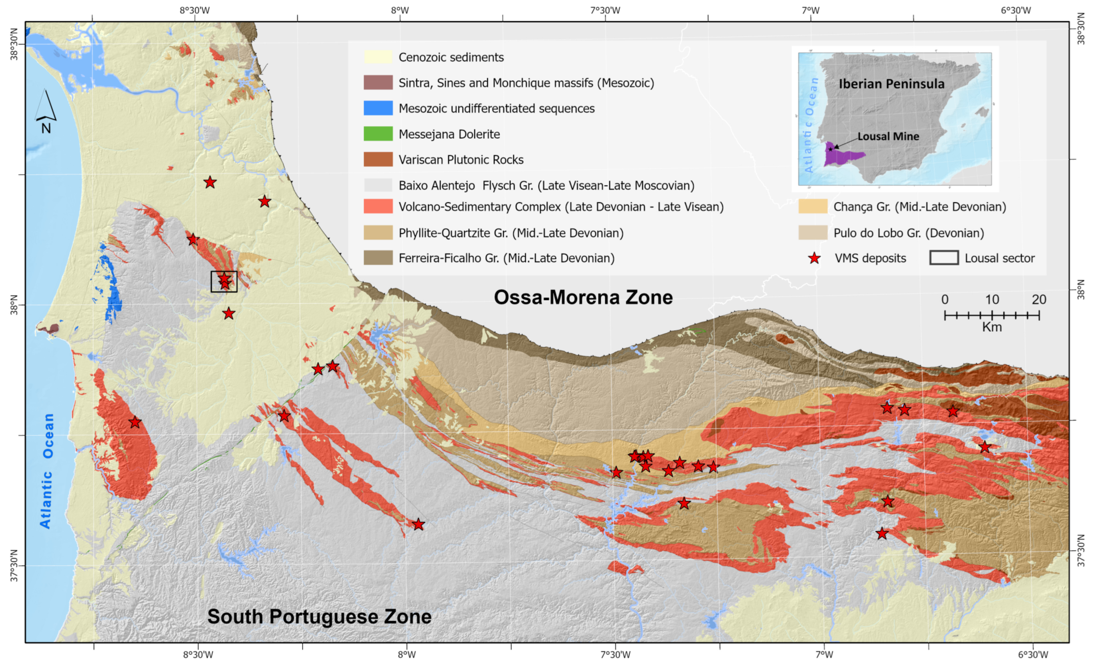
2. Lousal—A Brief History and Geological Setting

The Lousal mine (opened in 1900 and closed in 1988; the last owner was Mines et Industries (SAPEC)) is an old pyrite (FeS₂) mine located in Portugal in the NW sector of IPB (Figure 1), in a complex structure formed by the volcano–sedimentary complex (VSC) (Famennian to Visean age) and by the Phyllite–Quartzite Group (PQG) (Givetian to latest Famennian age—Strunian Biozone [28,30,31]), the two lithostratigraphic units of the IPB. The subvertical deposit was exploited by galleries to a ~500 m depth with a NW direction. It is a Volcanogenic Massive Sulphide (VMS) hosted in an antiform structure. Two main massive sulphide horizons can be considered in the Lousal antiform structure [28,29,32,33]: the western group formed by the extreme south, south and west sulphide lenses and the eastern group formed by the central, Miguel, José, Fernando, north, northeast and António sulphide lenses. The VSC host rocks of massive sulphide and stockwork mineralization are felsic volcanic rocks and black shales of the Lousal–Caveira Formation (Late Famennian age, [28,30,31]). Minor Cu-Au sulphide veins occur in the VSC and in the PQG.

The Lousal IPB mine has been rehabilitated by the Empresa de Desenvolvimento Mineiro in recent decades [28]. The mine facilities contain a Centro Ciência Viva and a Mining Museum [29].

3. Materials and Methods

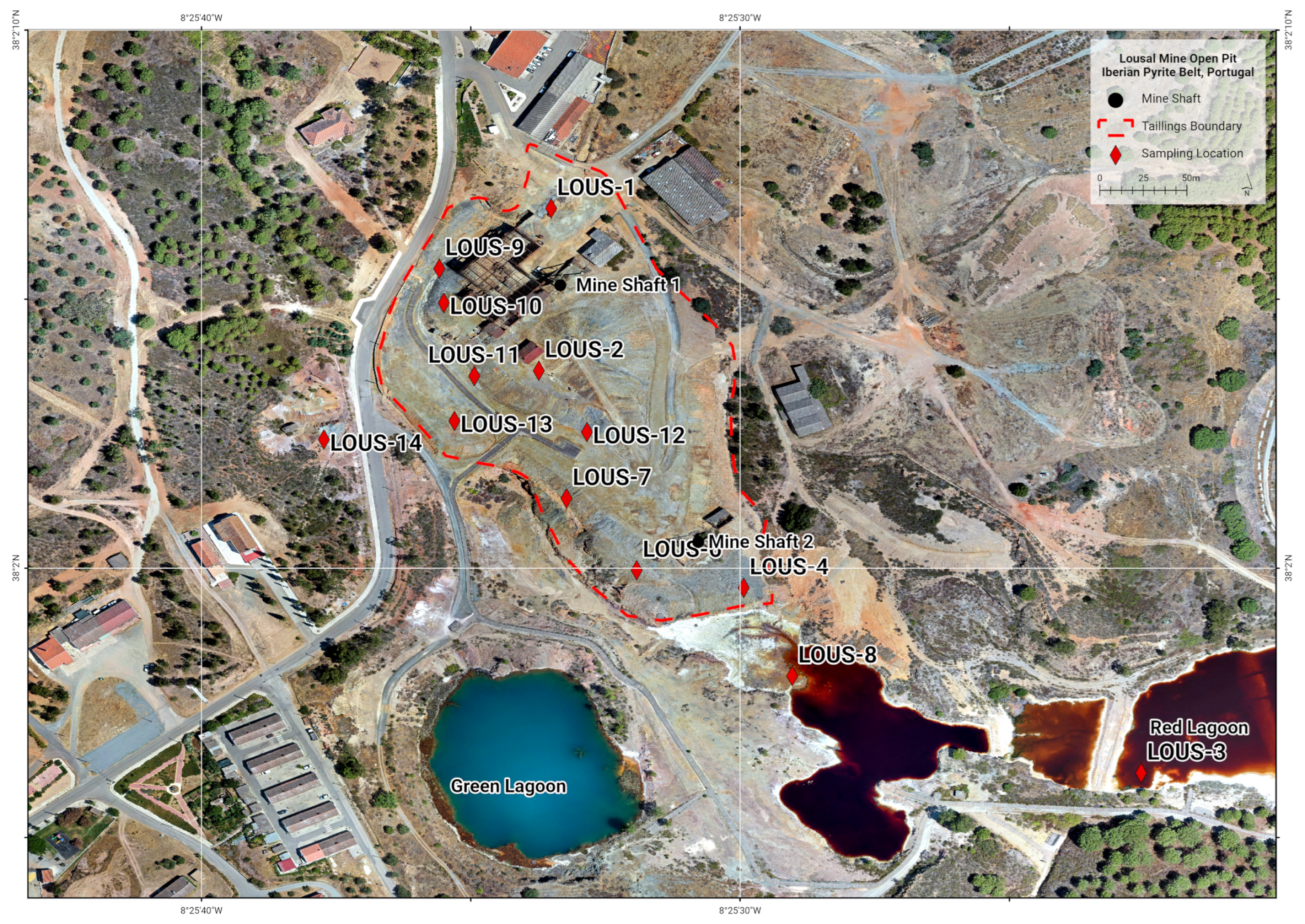
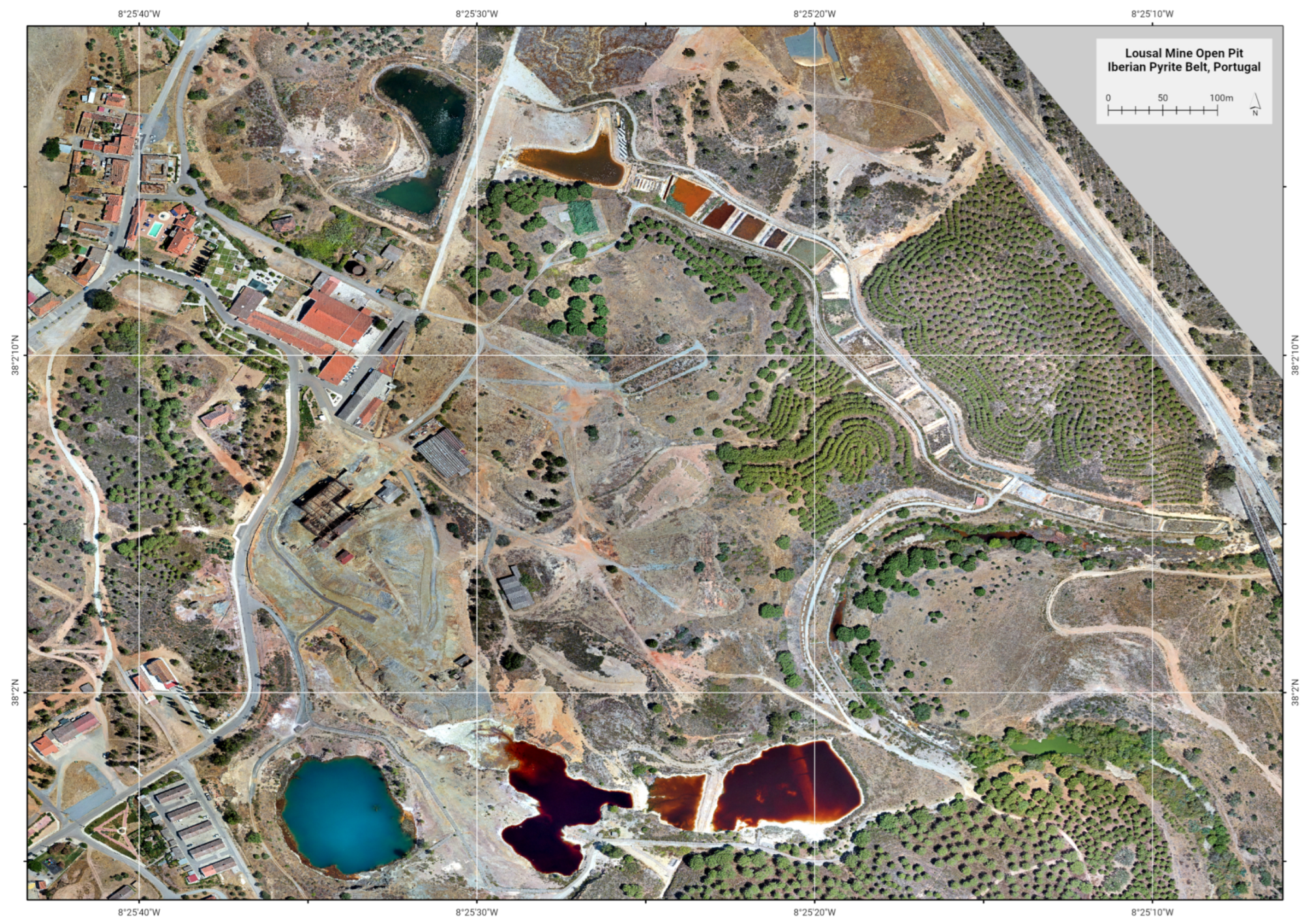
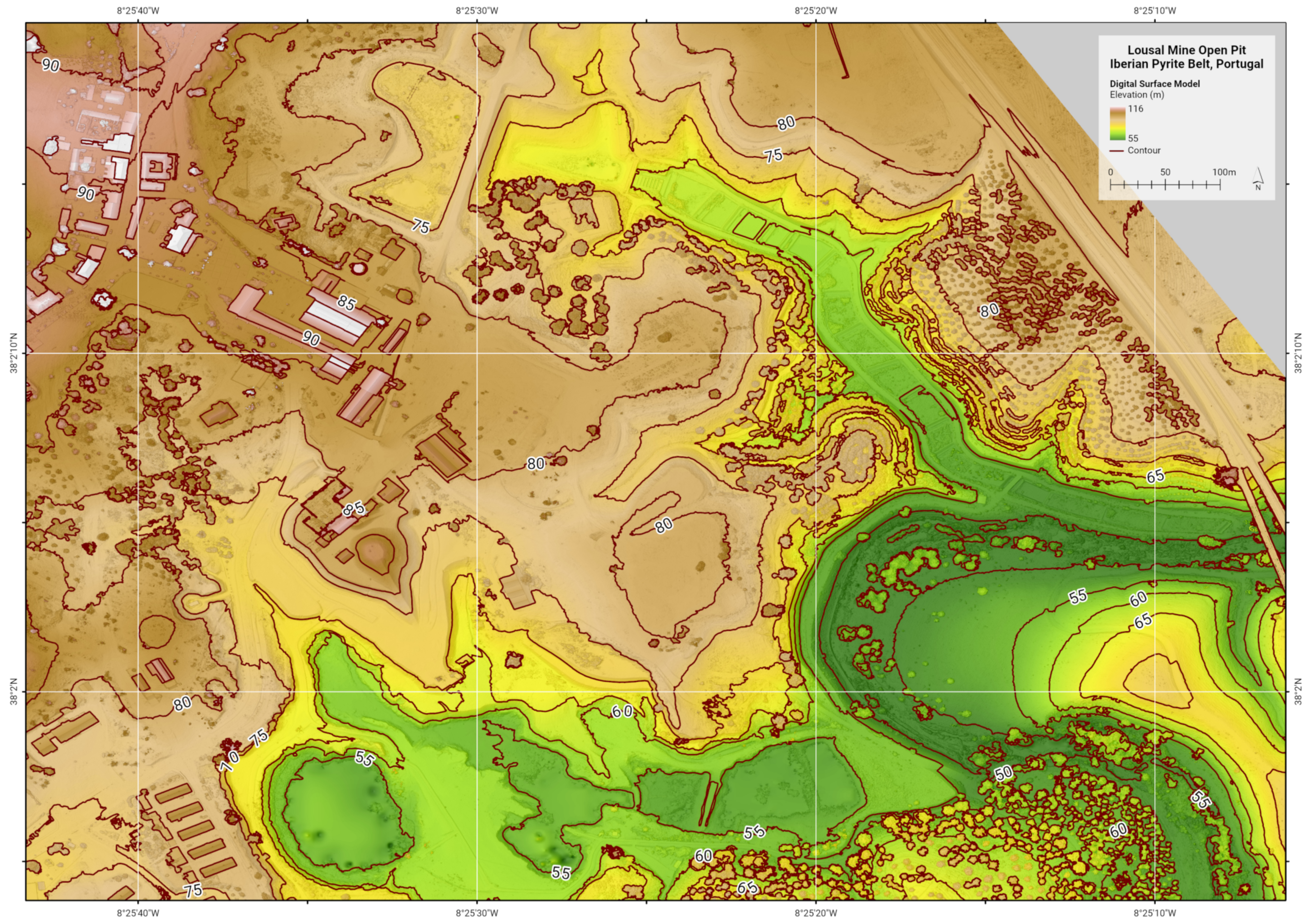
3.1. Waste Dump Mapping and Modelling

The Lousal mine is characterised by a large open pit with two lagoons flooded with acid mine water (pH < 3.9) [28,34,35,36]. The Green Lagoon is connected with the underground mine galleries while the Red Lagoon is characterised by ferric waters linked to an acid water spring (pH 3.3 to 2.4 [36]). The mine site is characterized by two main tailings areas [28]: a central area located near the mine shafts nº 1 and nº 2 and ore milling plant (original area of 23,907 m²) (Figure 2) and the NE area located near the railway siding (original area of 59,542 m²). Minor mine wastes are distributed in the south of the mine (in the left margin of the Corona stream), near the Miguel shaft and SE of shaft nº 2. The railway sector, to the north, includes milled ore.

The central area was modelled and studied in detail in the GSEU Project. Three waste types were considered through surface mapping [28]: (i) fine, milled sulphide ore (dimension < 2 cm) corresponding to the Lousal mine product (A-Class); (ii) ore (massive and stockwork mineralisation) + host rocks (felsic volcanic rocks and black shales) (<20 cm dimension) (B-Class); and (iii) dominant host rocks (<20 cm dimension) + sulphide ore blocks (<5 cm) (C-Class). The Lousal mine waste types reflect the simple ore treatment (ore crushing and minor choice of mineral selection) and the transport routes are by wagon, truck and later export by railway [28]. Unlike the IPB mines of São Domingos, Aljustrel and Caveira, in Lousal the ore was not roasted, so there was no waste slag.

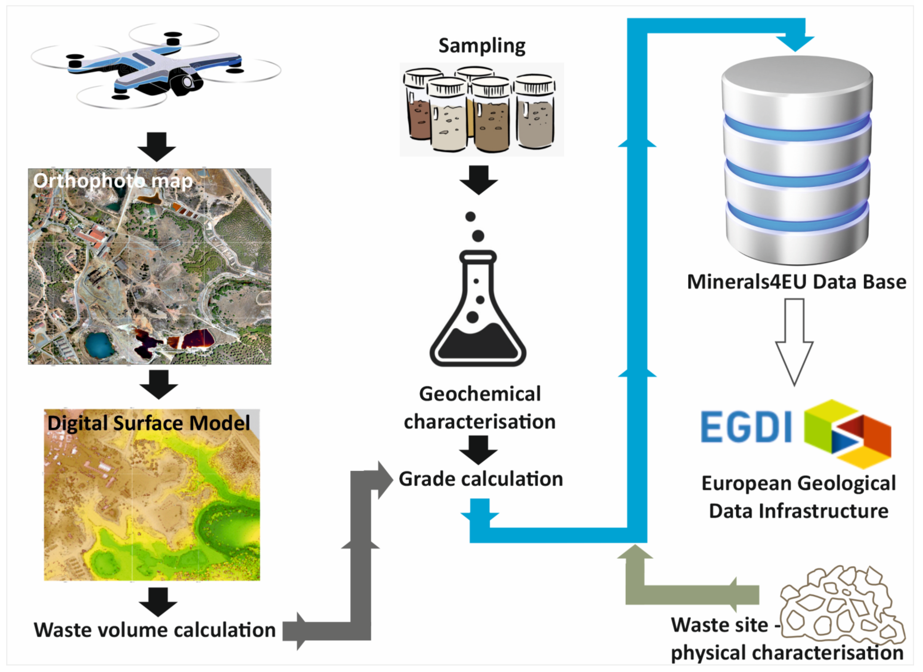
3.2. Methodology of Study

The general approach to reach the objectives of this study are generically shown in Figure 3. Each of these components will be further expanded below, but the process contains three main tasks running in parallel, namely, (i) the geological and mining survey upgrade and waste mapping [28], (ii) small Unmanned Aircraft System (sUAS) data acquisition and the photogrammetric reconstruction of the mine site and the mine waste selection (considering mine history and ore treatment) for the modelling phase and (iii) the physical characterization of the waste and samples. Each is handled separately to produce the various components needed and the two tasks join after the grade calculations (when possible) to incorporate the Minerals4EU database and subsequent upload to the European Geological Data Infrastructure (EGDI).

sUAS photogrammetry has increased in popularity in the geospatial industry [37] and enables the acquisition of imagery of a very high spatial and temporal resolution. The potential to reconstruct terrain using low-cost solutions such as sUAS [38] is of major interest to researchers in the earth sciences community [39].

3.3. Sample Treatment

A total of 13 samples were collected in locations that appeared to exhibit different types of mine waste (Figure 2). The variations included coarse- vs. fine-grained, the colour of the material and macroscopic mineralogy. At each sampling point, four individual samples were collected to make up a composite sample that was representative of the dump material at each point. The total sample collected was between 5 and 6 kg.

The samples for chemical analysis were initially dried and sieved by grain size: each sample was divided into 5 fractions and each fraction represented a sample for chemical analysis; for example, sample LOU/GSEU/002 gave rise to the following fractions:

• LOU/GSEU/002 as is (bulk sample);
• LOU/GSEU/002 < 4 mm and >3.35 mm;
• LOU/GSEU/002 < 3.35 mm and >2 mm;
• LOU/GSEU/002 < 2 mm and >500 µm;
• LOU/GSEU/002 < 500 µm and >250 µm.

A split was performed on each fraction and 200 g were removed for chemical analysis. These 200 g were fed in to feed the crusher (Retsch BB50 with tungsten jaws), which reduced the particle size of the fraction below 500 µm; this material was passed through a 75 µm sieve (grain size intended for chemical analysis) in order to better calibrate the sample for the agate mill (Retsch RS200) and reduce its size by removing material already with the intended grain size. After pulverization carried out in the agate mill, the sample wall sieved again through using a 75 µm sieve to be sure that the fraction is well calibrated.

A portable X-ray fluorescence (p-XRF) equipment, X-MET8000 Expert Geo from HITACHI, was used in the field for a rapid on-site chemical analysis when necessary, and for a chemical characterization of the powdered samples at the laboratory using a benchtop stand. This apparatus was equipped with a Rh tube (4 W) and a silicon drift detector (SDD). Measurements were made with a mining calibration including REE. The results were also compared with chemical analyses obtained by XRF (wavelength dispersive) laboratorial equipment (Philips PW2404) and through atomic absorption spectroscopy (Perkin Elmer, model PinAAcle 900T).

Powder X-ray diffraction data were collected using a D8 Advance Bruker AXS diffractometer (Bruker AXS GmbH, Karlsruhe, Germany) with Cu Kα radiation. The XRD data treatment was performed using DIFFRAC.EVA v5 software (Bruker AXS GmbH, Karlsruhe, Germany) (Bruker AXS DIFFRAC.EVA v5) for phase identification.

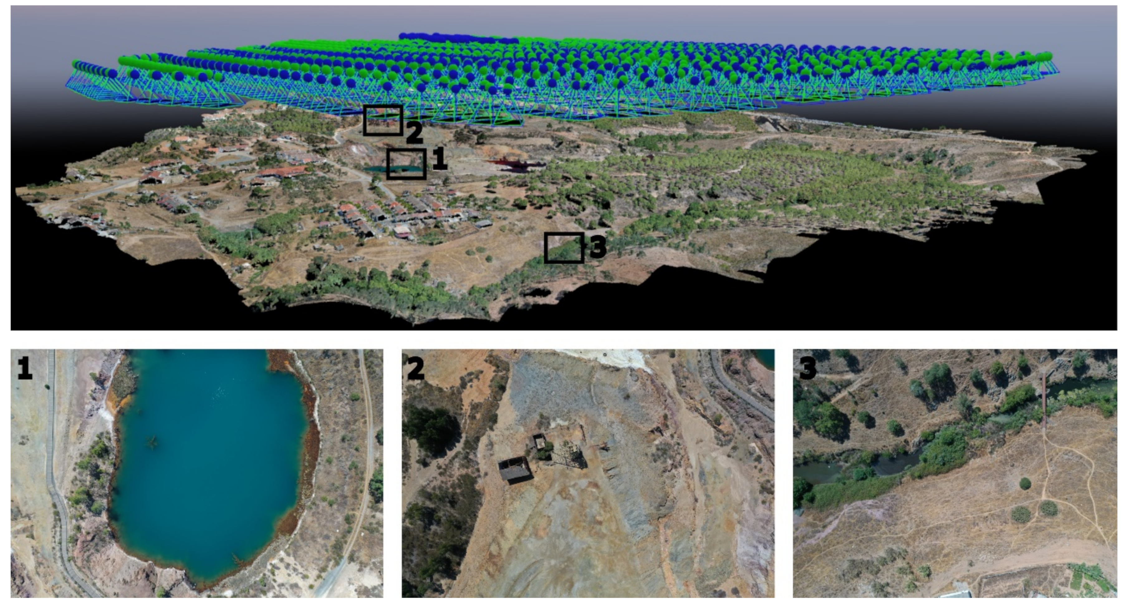
3.4. Aerial Data Acquisition

To create an orthomosaic image, a digital surface model (DSM) and digital terrain model (DTM) of the mine site, a low-cost multirotor sUAS solution for data acquisition was used. For this site in particular, because of its relatively small size, data acquisition was undertaken with a DJI Mavic 2 Pro equipped with a 20-megapixel Hasselblad camera sensor with electronic shutter. The flight was conducted in mid-2022, close to solar noon, to reduce the shadow effect of vegetation and buildings.

The flight area was drawn in Google Earth Pro and imported into the DJI Smart Controller. Using the DJI Pilot PE APP, the direction of flight and overlap for each flight were set and the mission was conducted in a grid pattern. Images were acquired with flight speeds at around 5 m per second and at a constant height of 100 m above ground level with 80% front lap and 80% side lap (

Table 1. Flight parameters for aerial image acquisition.

Parameter	Value
Flight Altitude (Above take-off)	100 m
Nº of images acquired	1105
Ground resolution of orthomosaic map	2.5 cm
Number of Flights	2
Total Flight Duration	60 min
Front Overlap	80%
Side Overlap	80%
Height Above Mean Sea Level	185 m
Area Covered	1.5 km2

).

4. Results

4.1. Aerial Data Acquisition and Processing

In total, 1105 photos were acquired, which were used to compute a high-resolution point cloud (Figure 4) an orthomosaic map with 2.5 cm/pixel (Figure 5) and both a digital surface model (Figure 6) and digital terrain model with 2.5/5 cm/pixel using a high-performance computer.

This study used Pix4D Mapper, version 4.4.12, which is a photogrammetric software that enables the user to create accurate 3D models and maps for a given location. The processing chain was divided in three main steps: (i) initial processing, which computes the position and orientation of aerial images relative to each other and the ground using the detection and matching of common features in overlapping images; (ii) point cloud generation, which computes 3D models such as a mesh and densified point cloud using multi-view-stereo algorithms [37,40]; and (iii) digital surface model and orthomosaic generation, which are computed based on the densified point cloud.

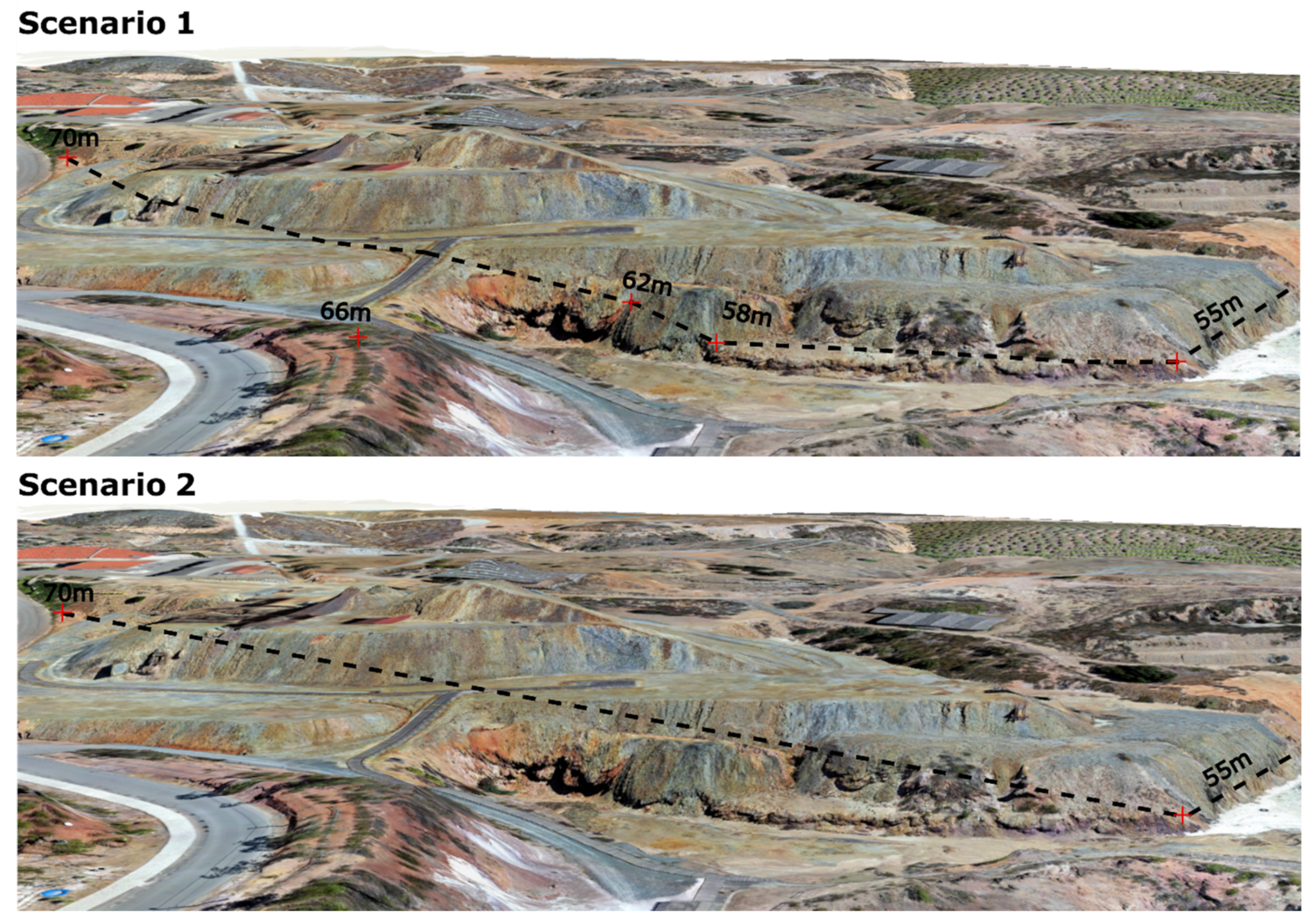
4.2. Mine Waste Volumes

As there is no historical information regarding the original topography of the mine site, to calculate the volume of the waste dump, two scenarios (Figure 7) were proposed to make an approximation to the original topography of where the main waste dump is located: Scenario 1, where the base surface was interpolated based on the maximum and minimum height of the outcrops; Scenario 2, where the height of the visible lateral outcrops was used to create contour lines at certain heights in order to better represent the original topography. Taking into account both possible scenarios, the results obtained were as follows: (a) Scenario 1, where the height of the visible lateral outcrops were used to create contour lines at certain heights in order to better represent what we assume is the original topography (result obtained: 322,455 m³), and (b) Scenario 2, where the base surface was interpolated based on the maximum and minimum height of the outcrops (result obtained: 308,478 m³).

For the surface information, data from the survey conducted with DJI Mavic 2 pro were used. These data allowed the creation of a very high resolution orthomosaic and digital surface model of the Lousal Mine with spatial resolution of 2.5 cm pixels. These high-resolution data enabled the construction of a digital terrain model of the mine with a spatial resolution of approximately 13 cm, where all the surface information regarding vegetation and man-made structures was removed.

To calculate the approximate volume of the waste dump, the original topography was subtracted from the current surface and the result was the volume contained between both surfaces.

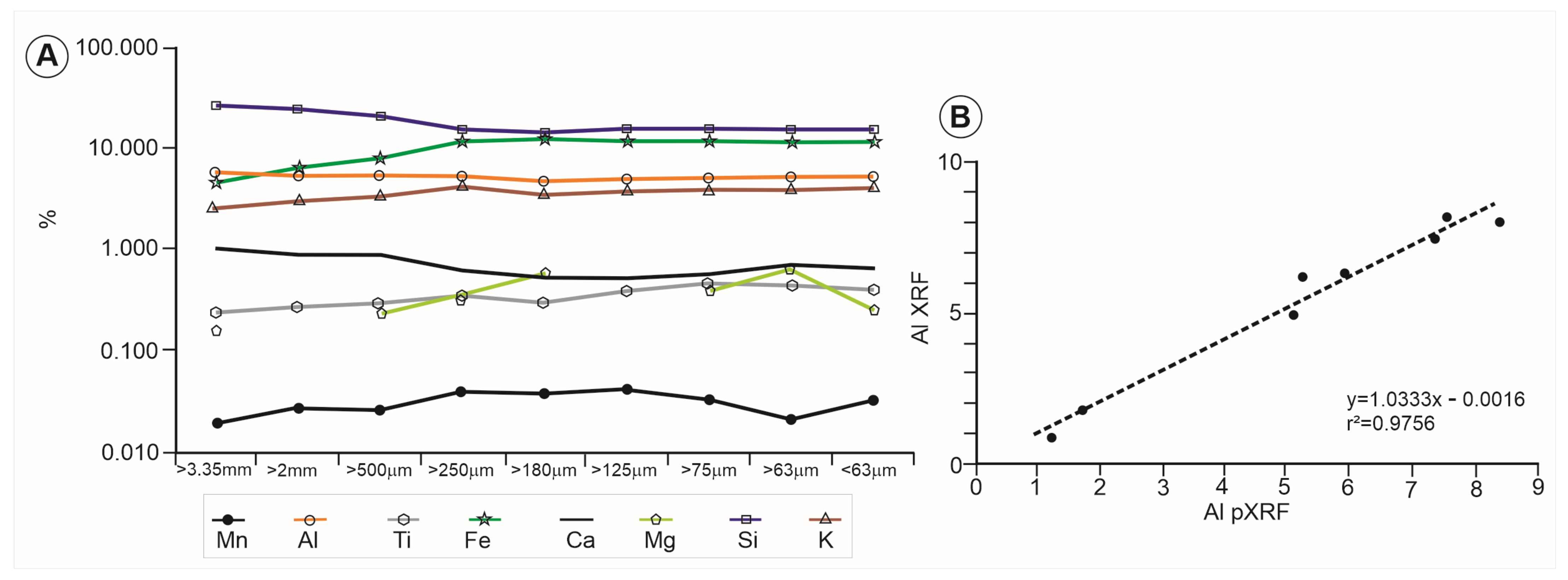
4.3. Geochemistry of Waste Materials

Chemical characterization was performed in the bulk sample and in each granulometric fraction (see Supplementary Materials Table S1), allowing us to observe in which sample a given element is more concentrated. As a first methodology to link it to a mineralogical phase or a carrier phase, without the need to resort to other more specialized and time-consuming techniques, like scanning electron microscopy (SEM), only some only those granulometric fractions with a higher content of the element of interest were chosen for XRD analysis. For instance, a higher content of lead was present in samples 1, 9, 10 and 14, while the critical raw materials (CRM) antimony and REE were more concentrated in samples 1, 10, 14 and 1, 9, 10, 12, respectively. Sample 8 was concentrated in several CRM (Co, Mg, Mn, and Sr) and in strategic raw materials (SRM) like Cu and Ni. Sample 14 was also rich in various CRMs (Sb, As, Bi, Nb, and Sr).

Due to the sample’s mineralogical complexity, only a semi-quantitative approach was performed to investigate the content of each phase. Phase identification was achieved through the analytical software, but also bearing in mind the elements previously identified by p-XRF (Supplementary Materials Table S1). XRD spectra of bulk samples can be seen in Supplementary Materials File S1. The mineralogy of these samples (

Table 2. Mineralogical phases identified by XRD (in alphabetical order for better visualization; symbols from IMA-CNMNC [41]). The main phases in each sample were roughly estimated as more (+++) or less (+) represented, through the intensity of the principal lines. Legend: Ab—Albite, Na(AlSi₃O₈); Acoq—Aluminocoquimbite, Al₂Fe₂(SO₄)₆(H₂O)₁₂·6H₂O; Agjrs—Argentojarosite, AgFe³⁺₃(SO₄)₂(OH)₆; Alg—Alunogen, Al₂(SO₄)₃·17H₂O; Alu—Alunite, KAl₃(SO₄)₂(OH)₆; Ang—Anglesite, PbSO₄; Anh—Anhydrite, CaSO₄; Apy—Arsenopyrite, FeAsS; Bdn—Beudantite, PbFe₃(AsO₄)(SO₄)(OH)₆; Bir—Birnessite, (Na,Ca)_0.5(Mn⁴⁺,Mn³⁺)₂O₄·1.5H₂O; Ccn—Cancrinite, (Na,Ca,◻)₈(Al₆Si₆O₂₄)(CO₃,SO₄)₂·2H₂O; Ccp—Chalcopyrite, CuFeS₂; Chm—Chamosite, (Fe²⁺)₅Al(Si,Al)₄O₁₀(OH,O)₈; Clc—Clinochlore, Mg₅Al(AlSi₃O₁₀)(OH)₈; Coq—Coquimbite, AlFe₃(SO₄)₆(H₂O)₁₂·6H₂O; Esm—Epsomite, MgSO₄·7H₂O; Fcpi—Ferricopiapite, Fe³⁺_0.67Fe³⁺₄(SO₄)₆(OH)₂·20H₂O; Gp—Gypsum, CaSO₄·2H₂O; Hhy—Hexahydrite, MgSO₄·6H₂O; Hth—Halotrichite, FeAl₂(SO₄)₄·22H₂O; Jrs—Jarosite, KFe³⁺₃(SO₄)₂(OH)₆; Kln—Kaolinite, Al₂(Si₂O₅)(OH)₄; Mcpi—Magnesiocopiapite, MgFe³⁺₄(SO₄)₆(OH)₂·20H₂O; Ms/Bt—Muscovite/Biotite, KAl₂(AlSi₃O₁₀)(OH)₂/K(Mg,Fe)₃AlSi₃O₁₀(OH)₂; Njrs—Natrojarosite, NaFe₃(SO₄)₂(OH)₆; Or—Orthoclase, K(AlSi₃O₈); Pbtl—Parabutlerite, Fe³⁺(SO₄)(OH)·2H₂O; Pcoq—Paracoquimbite, Fe₄(SO₄)₆(H₂O)₁₂·6H₂O;Phy—Pentahydrite, MgSO₄·5H₂O; Pjrs—Plumbojarosite, Pb_0.5Fe³⁺₃(SO₄)₂(OH)₆; Py—Pyrite, FeS₂; Qz—Quartz, SiO₂; Rbc—Rhomboclase, (H₅O₂)Fe³⁺(SO₄)₂·2H₂O; Röm—Römerite, Fe²⁺Fe³⁺₂(SO₄)₄·14H₂O; Rt—Rutile, TiO₂; S—Sulphur, S₈; Sd—Siderite, FeCO₃; Ske—Starkeyite, MgSO₄·4H₂O; Sp—Sphalerite, ZnS; Stn—Stannite, Cu₂FeSnS₄; Szo—Szomolnokite, FeSO₄·H₂O; Tmr—Tamarugite, NaAl(SO₄)₂·6H₂O; Vlt—Voltaite, K₂Fe²⁺₅Fe³⁺₃Al(SO₄)₁₂·18H₂O. Vtg: vestigial content; ?: dubious identification.

Sample Reference	Phase Identification	+++	++	+
LOUS/GSEU/001 Concentrated ore, A-Class	Ang + Anh + Coq + Gp + Hth? + Jrs + Ms/Bt (vtg) + Py + Qz + Rbc + Röm + S + Sp (vtg) + Stn + Vlt (vtg)	Pyrite, Quartz, Rhomboclase	Anhydrite, Anglesite	Coquimbite, Römerite, Gypsum, Jarosite
LOUS/GSEU/002; C-Class	Ab + Ccn? (vtg) + Gp + Jrs + Kln (vtg) + Ms/Bt + Njrs + Qz + Rbc	Quartz, Albite	Jarosite, Gypsum	Musc./Biotite
LOUS/GSEU/003; Red Lagoon Precipitate	Alu + Clc (vtg) + Esm + Gp + Hhy + Jrs + Ms/Bt + Njrs + Pbtl + Phy + Qz + Ske	Gypsum, Quartz	Musc./Biotite	Natrojarosite, Starkeyite
LOUS/GSEU/004; C-Class	Alu (vtg) + Chm + Gp + Jrs + Ms/Bt + Njrs + Qz + Rt	Quartz, Musc./Biotite	Chamosite, Gypsum	Jarosite
LOUS/GSEU/006; C-Class	Alu + Ang (vtg) + Chm + Gp + Jrs + Ms/Bt + Njrs + Or (vtg) + Qz + Rt	Quartz, Musc./Biotite, Gypsum, Chamosite	Jarosite
LOUS/GSEU/007; C-Class	Alu + Chm + Gp + Jrs + Ms/Bt + Njrs + Py + Qz + Rt + Sd	Quartz, Musc./Biotite, Chamosite	Jarosite
LOUS/GSEU/008; Red Lagoon Precipitate	Bir (vtg) + Ccp + Clc (vtg) + Gp + Hhy + Jrs + Ms/Bt + Njrs + Qz + Rt (vtg) + Ske + Sp (vtg) + Tmr	Quartz, Gypsum	Starkeyite, Hexahydrite, Tamarugite
LOUS/GSEU/009; B-Class	Ab + Ang + Ccp + Coq + Fcpi + Gp + Pcoq + Py + Qz + Rbc + Röm + Rt (vtg) + Sp + Szo + Vlt	Quartz, Pyrite, Coquimbite, Rhomboclase	Paracoquimbite, Ferricopiapite, Gypsum, Voltaite	Römerite, Szomolnokite, Albite, Anglesite
LOUS/GSEU/0010; C-Class	Ang + Ccp + Coq + Fcpi (vtg) + Ms/Bt + Njrs (vtg) + Pcoq + Py + Qz + Rbc + Röm + Sp + Szo + Vlt	Quartz, Rhomboclase	Römerite, Coquimbite, Pyrite	Paracoquimbite, Chalcopyrite, Anglesite
LOUS/GSEU/0011; C-Class	Ab + Acoq + Alg + Fcpi + Gp + Jrs + Ms/Bt + Qz + Rbc + Rt + Tmr	Quartz, Jarosite, Musc./Biotite, Ferricopiapite, Gypsum, Rhomboclase	Alunogen, Aluminocoquimbite, Tamarugite, Albite
LOUS/GSEU/0012; C-Class	Ang (vtg) + Apy ? + Ccp + Coq + Fcpi + Gp + Jrs + Ms/Bt (vtg) + Njrs + Py + Qz + Rbc + Röm (vtg) + Sp + Tmr	Quartz, Coquimbite	Rhomboclase, Ferricopiapite	Gypsum, Tamarugite
LOUS/GSEU/0013; C-Class	Alg (vtg) + Gp + Hth + Jrs + Mcpi + Ms/Bt + Njrs + Py + Qz + Rt	Quartz, Musc./Biotite	Gypsum, Jarosite, Magnesiocopiapite, Halotrichite
LOUS/GSEU/0014; C-Class	Agjrs + Ang + Bdn + Clc (vtg) + Coq + Fcpi + Jrs + Ms/Bt + Njrs + Pjrs + Qz + Rt + Sd	Quartz, Musc./Biotite	Ferricopiapite, Jarosite, Beudantite

) showed mainly the presence of pyrite, quartz, mica (like muscovite or biotite), feldspar (albite), and chlorite (chamosite), representing mineralization, host rocks with hydrothermal alteration (quartz, and feldspar + hydrothermal chlorite; [28]), and numerous neogenic sulphates related with supergene processes and weathering [28] with variable degrees of hydration, of which gypsum (CaSO₄·2H₂O), rhomboclase [(H₅O₂)Fe³⁺(SO₄)₂·2H₂O], ferricopiapite [Fe³⁺_0.67Fe³⁺₄(SO₄)₆(OH)₂·20H₂O], coquimbite [AlFe₃(SO₄)₆(H₂O)₁₂·6H₂O] and jarosite [KFe₃⁺³(SO₄)₂(OH)₆] stood out.

As said before, only those granulometric fractions from each sample with a higher content of an element of interest were chosen for XRD analysis. For example, for sample 1 (finely crushed ore, A-Class), a semi-quantitative approach of the content of each mineralogical phase was taken by comparing the intensity of the principal lines and attributing +++ to the granulometric fraction(s) with higher intensity for a given phase (

Table 3. Semi-quantitative approach of the mineralogical content of sample LOUS/GSEU/001. Legend: Ang—Anglesite, PbSO₄; Anh—Anhydrite, CaSO₄; Coq—Coquimbite, AlFe₃(SO₄)₆(H₂O)₁₂·6H₂O; Gp—Gypsum, CaSO₄·2H₂O; Hth—Halotrichite, FeAl₂(SO₄)₄·22H₂O; Jrs—Jarosite, KFe³⁺₃(SO₄)₂(OH)₆; Ms/Bt—Muscovite/Biotite, KAl₂(AlSi₃O₁₀)(OH)₂/K(Mg,Fe)₃AlSi₃O₁₀(OH)₂; Py—Pyrite, FeS₂; Qz—Quartz, SiO₂; Rbc—Rhomboclase, (H₅O₂)Fe³⁺(SO₄)₂·2H₂O; Röm—Römerite, Fe²⁺Fe³⁺₂(SO₄)₄·14H₂O; S—Sulphur, S₈; Sp—Sphalerite, ZnS; Stn—Stannite, Cu₂FeSnS₄; Vlt—Voltaite, K₂Fe²⁺₅Fe³⁺₃Al(SO₄)₁₂·18H₂O. Vtg: vestigial content; -: not detected; ?: dubious identification.

Sample Reference	Granulometry	Ang	Anh	Coq	Gp	Hth ?	Jrs	Ms/Bt	Py	Qz	Rbc	Röm	S	Sp	Stn	Vlt
LOUS/GSEU/001	Bulk sample	+++	++	++	++	+++	+++	Vtg	+++	++	++	+++	++	Vtg	+++	Vtg
	>3.35 mm	++	-	Vtg	++	+++	-	Vtg	+++	+++	-	Vtg	+	Vtg	+++	Vtg
	>250 μm	+++	++	+++	+++	++	-	Vtg	+++	++	+++	+++	+++	Vtg	+++	-
	>180 μm	++	++	+++	-	+++	Vtg	Vtg	++	+++	++	++	++	Vtg	++	Vtg
	>63 μm	++	+++	Vtg	-	++	-	Vtg	+++	+	+	-	+	Vtg	+++	-

). The medium, low, or very low intensity of the principal lines of the phase was classified as ++, + or vtg (vestigial content), respectively.

Table 4. Semi-quantitative approach of the mineralogical content of sample LOUS/GSEU/002. Legend: Ab—Albite, Na(AlSi₃O₈); Ccn—Cancrinite, (Na,Ca,◻)₈(Al₆Si₆O₂₄)(CO₃,SO₄)₂·2H₂O; Gp—Gypsum, CaSO₄·2H₂O; Jrs—Jarosite, KFe³⁺₃(SO₄)₂(OH)₆; Kln—Kaolinite, Al₂(Si₂O₅)(OH)₄; Ms/Bt—Muscovite/Biotite, KAl₂(AlSi₃O₁₀)(OH)₂/K(Mg,Fe)₃AlSi₃O₁₀(OH)₂; Njrs—Natrojarosite, NaFe₃(SO₄)₂(OH)₆; Qz—Quartz, SiO₂; Rbc—Rhomboclase, (H₅O₂)Fe³⁺(SO₄)₂·2H₂O. Vtg: vestigial content; -: not detected; ?: dubious identification.

Sample Reference	Granulometry	Ab	Ccn ?	Gp	Jrs	Kln	Ms/Bt	Njrs	Qz	Rbc
LOUS/GSEU/002	Bulk sample	++	Vtg	+++	+++	Vtg	++	++	+	++
	>3.35 mm	+++	Vtg	+++	+++	Vtg	+++	++	+++	Vtg
	>180 μm	+	Vtg	++	+++	-	++	+++	+	+++

,

Table 5. Semi-quantitative approach of the mineralogical content of sample LOUS/GSEU/003. Legend: Alu—Alunite, KAl₃(SO₄)₂(OH)₆; Clc—Clinochlore, Mg₅Al(AlSi₃O₁₀)(OH)₈; Esm—Epsomite, MgSO₄·7H₂O; Gp—Gypsum, CaSO₄·2H₂O; Hhy—Hexahydrite, MgSO₄·6H₂O; Jrs—Jarosite, KFe³⁺₃(SO₄)₂(OH)₆; Ms/Bt—Muscovite/Biotite, KAl₂(AlSi₃O₁₀)(OH)₂/K(Mg,Fe)₃AlSi₃O₁₀(OH)₂; Njrs—Natrojarosite, NaFe₃(SO₄)₂(OH)₆; Pbtl—Parabutlerite, Fe³⁺(SO₄)(OH)·2H₂O; Phy—Pentahydrite, MgSO₄·5H₂O; Qz—Quartz, SiO₂; Ske—Starkeyite, MgSO₄·4H₂O. Vtg: vestigial content.

Sample Reference	Granulometry	Alu	Clc	Esm	Gp	Hhy	Jrs	Ms/Bt	Njrs	Pbtl	Phy	Qz	Ske
LOUS/GSEU/003	Bulk sample	+++	Vtg	++	+	++	++	+++	+++	++	++	+++	+++
	>3.35 mm	++	Vtg	+++	+	+	+	++	++	+	+	+++	+
	>75 μm	++	Vtg	++	+++	+++	+++	+	++	+++	+++	++	+++

,

Table 6. Semi-quantitative approach of the mineralogical content of sample LOUS/GSEU/004. Legend: Alu—Alunite, KAl₃(SO₄)₂(OH)₆; Chm—Chamosite, (Fe²⁺)₅Al(Si,Al)₄O₁₀(OH,O)₈; Gp—Gypsum, CaSO₄·2H₂O; Jrs—Jarosite, KFe³⁺₃(SO₄)₂(OH)₆; Ms/Bt—Muscovite/Biotite, KAl₂(AlSi₃O₁₀)(OH)₂/K(Mg,Fe)₃AlSi₃O₁₀(OH)₂; Njrs—Natrojarosite, NaFe₃(SO₄)₂(OH)₆; Qz—Quartz, SiO₂; Rt—Rutile, TiO₂. Vtg: vestigial content.

Sample Reference	Granulometry	Alu	Chm	Gp	Jrs	Ms/Bt	Njrs	Qz	Rt
LOUS/GSEU/004	Bulk sample	Vtg	+++	+++	+++	+++	+++	+++	+++
	>3.35 mm	Vtg	+++	+	++	+++	++	++	+++

,

Table 7. Semi-quantitative approach of the mineralogical content of sample LOUS/GSEU/006. Alu—Alunite, KAl₃(SO₄)₂(OH)₆; Ang—Anglesite, PbSO₄; Chm—Chamosite, (Fe²⁺)₅Al(Si,Al)₄O₁₀(OH,O)₈; Gp—Gypsum, CaSO₄·2H₂O; Jrs—Jarosite, KFe³⁺₃(SO₄)₂(OH)₆; Ms/Bt—Muscovite/Biotite, KAl₂(AlSi₃O₁₀)(OH)₂/K(Mg,Fe)₃AlSi₃O₁₀(OH)₂; Njrs—Natrojarosite, NaFe₃(SO₄)₂(OH)₆; Or—Orthoclase, K(AlSi₃O₈); Qz—Quartz, SiO₂; Rt—Rutile, TiO₂. Vtg: vestigial content.

Sample Reference	Granulometry	Alu	Ang	Chm	Gp	Jrs	Ms/Bt	Njrs	Or	Qz	Rt
LOUS/GSEU/006	Bulk sample	+++	Vtg	+++	+++	+++	+++	++	Vtg	+++	+++
	>3.35 mm	+++	Vtg	+++	++	++	+++	++	Vtg	+++	+++

,

Table 8. Semi-quantitative approach of the mineralogical content of sample LOUS/GSEU/007. Alu—Alunite, KAl₃(SO₄)₂(OH)₆; Chm—Chamosite, (Fe²⁺)₅Al(Si,Al)₄O₁₀(OH,O)₈; Gp—Gypsum, CaSO₄·2H₂O; Jrs—Jarosite, KFe³⁺₃(SO₄)₂(OH)₆; Ms/Bt—Muscovite/Biotite, KAl₂(AlSi₃O₁₀)(OH)₂/K(Mg,Fe)₃AlSi₃O₁₀(OH)₂; Njrs—Natrojarosite, NaFe₃(SO₄)₂(OH)₆; Py—Pyrite, FeS₂; Qz—Quartz, SiO₂; Rt—Rutile, TiO₂; Sd—Siderite, FeCO₃.

Sample Reference	Granulometry	Alu	Chm	Gp	Jrs	Ms/Bt	Njrs	Py	Qz	Rt	Sd
LOUS/GSEU/007	Bulk sample	+++	++	+++	+++	++	+++	+++	+	+	++
	>3.35 mm	+++	+++	++	++	+++	++	++	+++	+++	+++

,

Table 9. Semi-quantitative approach of the mineralogical content of sample LOUS/GSEU/008. Bir—Birnessite, (Na,Ca)_0.5(Mn⁴⁺,Mn³⁺)₂O₄·1.5H₂O; Ccp—Chalcopyrite, CuFeS₂; Clc—Clinochlore, Mg₅Al(AlSi₃O₁₀)(OH)₈; Gp—Gypsum, CaSO₄·2H₂O; Hhy—Hexahydrite, MgSO₄·6H₂O; Jrs—Jarosite, KFe³⁺₃(SO₄)₂(OH)₆; Ms/Bt—Muscovite/Biotite, KAl₂(AlSi₃O₁₀)(OH)₂/K(Mg,Fe)₃AlSi₃O₁₀(OH)₂; Njrs—Natrojarosite, NaFe₃(SO₄)₂(OH)₆; Qz—Quartz, SiO₂; Rt—Rutile, TiO₂; Ske—Starkeyite, MgSO₄·4H₂O; Sp—Sphalerite, ZnS; Tmr—Tamarugite, NaAl(SO₄)₂·6H₂O. Vtg: vestigial content.

Sample Reference	Granulometry	Bir	Ccp	Clc	Gp	Hhy	Jrs	Ms/Bt	Njrs	Qz	Rt	Ske	Sp	Tmr
LOUS/GSEU/008	Bulk sample	Vtg	Vtg	Vtg	+	+	+	+	+	++	Vtg	++	Vtg	++
	>3.35 mm	Vtg	Vtg	Vtg	+	+	+	++	+	++	Vtg	++	Vtg	++
	>250 μm	Vtg	Vtg	Vtg	+	++	+++	+++	+++	+++	Vtg	+++	Vtg	+++
	>75 μm	Vtg	+++	Vtg	+++	+++	+	+++	+	+	Vtg	Vtg	Vtg	++

,

Table 10. Semi-quantitative approach of the mineralogical content of sample LOUS/GSEU/009. Legend: Ab—Albite, Na(AlSi₃O₈); Ang—Anglesite, PbSO₄; Ccp—Chalcopyrite, CuFeS₂; Coq—Coquimbite, AlFe₃(SO₄)₆(H₂O)₁₂·6H₂O; Fcpi—Ferricopiapite, Fe³⁺_0.67Fe³⁺₄(SO₄)₆(OH)₂·20H₂O; Gp—Gypsum, CaSO₄·2H₂O; Pcoq—Paracoquimbite, Fe₄(SO₄)₆(H₂O)₁₂·6H₂O; Py—Pyrite, FeS₂; Qz—Quartz, SiO₂; Rbc—Rhomboclase, (H₅O₂)Fe³⁺(SO₄)₂·2H₂O; Röm—Römerite, Fe²⁺Fe³⁺₂(SO₄)₄·14H₂O; Rt—Rutile, TiO₂; Sp—Sphalerite, ZnS; Szo—Szomolnokite, FeSO₄·H₂O; Vlt—Voltaite, K₂Fe²⁺₅Fe³⁺₃Al(SO₄)₁₂·18H₂O. Vtg: vestigial content; -: not detected.

Sample Reference	Granulometry	Ab	Ang	Ccp	Coq	Fcpi	Gp	Pcoq	Py	Qz	Rbc	Röm	Rt	Sp	Szo	Vlt
LOUS/GSEU/009	Bulk sample	++	+	+++	+++	++	+++	++	+	++	+	++	-	+	+++	++
	>3.35 mm	++	-	+++	+++	++	-	-	+	+++	+	+++	-	++	++	++
	>2 mm	++	-	+++	+++	+++	++	Vtg	+	++	+++	+++	-	+++	++	+++
	>500 μm	+++	-	+++	+++	+++	++	-	+	++	++	++	-	++	++	+++
	<63 μm	+	+++	+++	++	++	+++	+++	+++	++	-	++	Vtg	Vtg	+++	Vtg

,

Table 11. Semi-quantitative approach of the mineralogical content of sample LOUS/GSEU/010. Legend: Ang—Anglesite, PbSO₄; Ccp—Chalcopyrite, CuFeS₂; Coq—Coquimbite, AlFe₃(SO₄)₆(H₂O)₁₂·6H₂O; Fcpi—Ferricopiapite, Fe³⁺_0.67Fe³⁺₄(SO₄)₆(OH)₂·20H₂O; Ms/Bt—Muscovite/Biotite, KAl₂(AlSi₃O₁₀)(OH)₂/K(Mg,Fe)₃AlSi₃O₁₀(OH)₂; Njrs—Natrojarosite, NaFe₃(SO₄)₂(OH)₆; Pcoq—Paracoquimbite, Fe₄(SO₄)₆(H₂O)₁₂·6H₂O; Py—Pyrite, FeS₂; Qz—Quartz, SiO₂; Rbc—Rhomboclase, (H₅O₂)Fe³⁺(SO₄)₂·2H₂O; Röm—Römerite, Fe²⁺Fe³⁺₂(SO₄)₄·14H₂O; Sp—Sphalerite, ZnS; Szo—Szomolnokite, FeSO₄·H₂O; Vlt—Voltaite, K₂Fe²⁺₅Fe³⁺₃Al(SO₄)₁₂·18H₂O. Vtg: vestigial content; -: not detected.

Sample Reference	Granulometry	Ang	Ccp	Coq	Fcpi	Ms/Bt	Njrs	Pcoq	Py	Qz	Rbc	Röm	Sp	Szo	Vlt
LOUS/GSEU/010	Bulk sample	++	++	++	Vtg	+	Vtg	++	++	+++	++	+++	+++	++	++
	>3.35 mm	Vtg	+	+	Vtg	-	Vtg	+	+	+++	+++	++	++	++	+++
	>180 μm	++	+++	+++	Vtg	+	Vtg	++	+++	+++	++	+++	+++	+++	++
	<63 μm	+++	+	++	Vtg	+	Vtg	+++	++	++	++	++	Vtg	++	++

,

Table 12. Semi-quantitative approach of the mineralogical content of sample LOUS/GSEU/011. Legend: Ab—Albite, Na(AlSi3O₈); Acoq—Aluminocoquimbite, Al₂Fe₂(SO₄)₆(H₂O)₁₂·6H₂O; Alg—Alunogen, Al₂(SO₄)₃·17H₂O; Fcpi—Ferricopiapite, Fe³⁺_0.67Fe³⁺₄(SO₄)₆(OH)₂·20H₂O; Gp—Gypsum, CaSO₄·2H₂O; Jrs—Jarosite, KFe³⁺₃(SO₄)₂(OH)₆; Ms/Bt—Muscovite/Biotite, KAl₂(AlSi₃O₁₀)(OH)₂/K(Mg,Fe)₃AlSi₃O₁₀(OH)₂; Qz—Quartz, SiO₂; Rbc—Rhomboclase, (H₅O₂)Fe³⁺(SO₄)₂·2H₂O; Rt—Rutile, TiO₂; Tmr—Tamarugite, NaAl(SO₄)₂·6H₂O.

Sample Reference	Granulometry	Ab	Acoq	Alg	Fcpi	Gp	Jrs	Ms/Bt	Qz	Rbc	Rt	Tmr
LOUS/GSEU/011	Bulk sample	++	+++	++	++	+++	+++	+++	+++	+++	+++	+++
	>3.35 mm	+++	+++	+++	+++	++	++	+++	++	+++	+++	+++

,

Table 13. Semi-quantitative approach of the mineralogical content of sample LOUS/GSEU/012. Legend: Ang—Anglesite, PbSO₄; Apy—Arsenopyrite, FeAsS; Ccp—Chalcopyrite, CuFeS₂; Coq—Coquimbite, AlFe₃(SO₄)₆(H₂O)₁₂·6H₂O; Fcpi—Ferricopiapite, Fe³⁺_0.67Fe³⁺₄(SO₄)₆(OH)₂·20H₂O; Gp—Gypsum, CaSO₄·2H₂O; Jrs—Jarosite, KFe³⁺₃(SO₄)₂(OH)₆; Ms/Bt—Muscovite/Biotite, KAl₂(AlSi₃O₁₀)(OH)₂/K(Mg,Fe)₃AlSi₃O₁₀(OH)₂; Njrs—Natrojarosite, NaFe₃(SO₄)₂(OH)₆; Py—Pyrite, FeS₂; Qz—Quartz, SiO₂; Rbc—Rhomboclase, (H₅O₂)Fe³⁺(SO₄)₂·2H₂O; Röm—Römerite, Fe²⁺Fe³⁺₂(SO₄)₄·14H₂O; Sp—Sphalerite, ZnS; Tmr—Tamarugite, NaAl(SO₄)₂·6H₂O. Vtg: vestigial content; -: not detected; ?: dubious identification.

Sample Reference	Granulometry	Ang	Apy ?	Ccp	Coq	Fcpi	Gp	Jrs	Ms/Bt	Njrs	Py	Qz	Rbc	Röm	Sp	Tmr
LOUS/GSEU/012	Bulk sample	-	Vtg	++	++	++	+++	++	Vtg	++	+++	+++	++	Vtg	++	++
	>3.35 mm	Vtg	Vtg	++	+++	+++	++	+++	Vtg	+++	++	++	+++	Vtg	++	++
	>500 μm	-	Vtg	+++	++	++	++	++	Vtg	++	++	++	++	Vtg	+++	+++

,

Table 14. Semi-quantitative approach of the mineralogical content of sample LOUS/GSEU/013. Legend: Alg—Alunogen, Al₂(SO₄)₃·17H₂O; Gp—Gypsum, CaSO₄·2H₂O; Hth—Halotrichite, FeAl₂(SO₄)₄·22H₂O; Jrs—Jarosite, KFe³⁺₃(SO₄)₂(OH)₆; Mcpi—Magnesiocopiapite, MgFe³⁺₄(SO₄)₆(OH)₂·20H₂O; Ms/Bt—Muscovite/Biotite, KAl₂(AlSi₃O₁₀)(OH)₂/K(Mg,Fe)₃AlSi₃O₁₀(OH)₂; Njrs—Natrojarosite, NaFe₃(SO₄)₂(OH)₆; Py—Pyrite, FeS₂; Qz—Quartz, SiO₂; Rt—Rutile, TiO₂. Vtg: vestigial content.

Sample Reference	Granulometry	Alg	Gp	Hth	Jrs	Mcpi	Ms/Bt	Njrs	Py	Qz	Rt
LOUS/GSEU/013	Bulk sample	Vtg	+++	+++	+++	+++	+++	+++	++	+++	+++
	>3.35 mm	Vtg	+	++	++	++	+	++	+++	+++	++

and

Table 15. Semi-quantitative approach of the mineralogical content of sample LOUS/GSEU/014. Legend: Agjrs—Argentojarosite, AgFe₃⁺³(SO₄)₂(OH)₆; Ang—Anglesite, PbSO₄; Bdn—Beudantite, PbFe₃(AsO₄)(SO₄)(OH)₆; Clc—Clinochlore, Mg₅Al(AlSi₃O₁₀)(OH)₈; Coq—Coquimbite, AlFe₃(SO₄)₆(H₂O)₁₂·6H₂O; Fcpi—Ferricopiapite, Fe³⁺_0.67Fe³⁺₄(SO₄)₆(OH)₂·20H₂O; Jrs—Jarosite, KFe³⁺₃(SO₄)₂(OH)₆; Ms/Bt—Muscovite/Biotite, KAl₂(AlSi₃O₁₀)(OH)₂/K(Mg,Fe)₃AlSi₃O₁₀(OH)₂; Njrs—Natrojarosite, NaFe₃(SO₄)₂(OH)₆; Pjrs—Plumbojarosite, Pb_0.5Fe³⁺₃(SO₄)₂(OH)₆; Qz—Quartz, SiO₂; Rt—Rutile, TiO₂; Sd—Siderite, FeCO₃. Vtg: vestigial content.

Sample Reference	Granulometry	Agjrs	Ang	Bdn	Clc	Coq	Fcpi	Jrs	Ms/Bt	Njrs	Pjrs	Qz	Rt	Sd
LOUS/GSEU/014	Bulk sample	++	+	++	Vtg	+	+++	++	+++	+++	+++	+	++	++
	>3.35 mm	++	Vtg	++	Vtg	+	+++	+++	+++	+++	+	+++	++	+++
	>180 μm	++	+	++	Vtg	+++	+++	+	+	++	+++	+	+++	++
	>75 μm	++	++	+++	Vtg	+++	+++	++	++	++	+	+	+++	++
	<63 μm	+++	+++	++	Vtg	++	++	+	++	++	++	+	+++	++

were constructed with the same methodology.

Anglesite (Ang) was the main lead mineral identified in samples 1, 6, 9, 10 and 12 (Table 3, Table 7, Table 10, Table 11 and Table 13), but in sample 14, with the highest content of Pb (about 3%) and As (about 2%) (Table 2), two more Pb-minerals were present, beudantite (Bdn) and plumbojarosite (Pjrs), with beudantite being very well represented (Table 2 and Table 15), justifying the high level of As and probably representing the alteration of arsenopyrite.

Stannite (Stn), although common in the IPB, e.g., ref. [28], was the unique Sn-mineral present in the Lousal samples, only identified in sample 1 (finely crushed ore, A-Class; Table 2 and Table 3), with a tin content of about 0.1%. Nevertheless, sample 10 had the same tin content, and sample 14 had about 0.2% (Table S1).

Several Mg minerals were recognized in these samples, mainly in samples 3 and 8 with Mg contents around 3% and 4%, respectively (Table S1), namely starkeyite (Ske), hexahydrite (Hhy), magnesiocopiapite (Mcpi), epsomite (Esm), pentahydrate (Phy) and clinochlore (Clc) (Table 5, Table 9 and Table 10). The majority are simple magnesium sulphates with various degrees of hydration. The same samples presented the highest level of Mn, 0.7% and 1.2%, respectively, with the mineral birnessite (Bir) being identified only in sample 8 (Table 2 and Table 9). The highest content of Co and Ni was achieved in the fraction > 75 μm, in samples 3 and 8, and could be related to the presence of gypsum, hexahydrite or even chalcopyrite (Ccp) (Table 5 and Table 9).

Rutile (Rt) and sphalerite (Sp) appeared in various samples (4, 6, 7, 9, 11, 13, 14 and 12, respectively), in which the highest Ti and Zn-contents were about 0.5% and 1%, respectively, and chalcopyrite contained approximately 0.6% Cu in sample 12.

Alunite [(K,Na)Al₃(SO₄)₂(OH)₆] (Alu) and jarosite [KFe₃(SO₄)₂(OH)₆] (Jrs) belong to the alunite supergroup, with the general formula AB₃(SO₄)₂(OH)₆ (A = K⁺, Na⁺, plus minor Ag⁺, Tl⁺, NH₄⁺, Pb²⁺, Bi³⁺, and B = Al³⁺ or Fe³⁺, respectively, in the subgroups of alunite and jarosite) [42]). Alunite only appeared in samples 3, 4, 6 and 7 (Table 2) and was poorly represented. This mineral occurred in the southern area of the Lousal open pit near the Central orebody gossan [28]. Jarosite or natrojarosite (Njrs) were well represented in almost all Lousal samples. Samples 1 and 14 had around 130 ppm and 160 ppm of Ag, respectively, with argentojarosite (Agjrs) being identified in the last sample. Plumbojarosite also appeared in sample 14 as already mentioned, in which Bi had an average content around 480 ppm. Bismuth could be probably found in plumbojarosite when comparing the semi-quantitative approach for this phase in the granulometric fractions (Table 15) with the Bi content (Table S1). These sulphates could be supergenic and related to VMS mineralization alteration by weathering [28].

Sulphates of the copiapite group include mixed-valence minerals with the general formula A²⁺Fe³⁺₄(SO₄)₆(OH)₂·20H₂O, where in A = Ca, Cu, Fe (copiapite s.s.), Mg (magnesiocopiapite), Zn, and trivalent minerals with general formula B³⁺_2/3Fe³⁺₄(SO₄)₆(OH)₂·20H₂O, wherein B = Al, Fe (ferricopiapite, Fcpi) [43]. Ferricopiapite was well represented in samples 9, 11, 12 and 14 and magnesiocopiapite in sample 13.

Coquimbite (Coq), aluminocoquimbite (Acoq) and paracoquimbite (Pcoq) were well represented in samples 1, 9, 10, 11 and 12 (Table 2), being the highest value of Ga (about 40 ppm) attained for samples 9 and 10, probably due to the presence of sphalerite (Table 10 and Table 11).

4.3.1. Evaluation of the Secondary Resources of the Lousal Waste Dump

Oxides of Major Elements

For a better evaluation of the secondary resources, the chemical analyses of the bulk samples obtained through the portable equipment of XRF (Table S1) were compared with those obtained with the laboratorial equipment (

Table 16. Major and minor element results of laboratory-analysed samples by XRF; * sample impossible to fuse due to high content of sulphides (iron content obtained by atomic absorption spectroscopy). Major element results in % and minor element results in ppm, unless otherwise stated.

Element	LOUS/ GSEU/ 001	LOUS/ GSEU/ 002	LOUS/ GSEU/ 004	LOUS/ GSEU/ 006	LOUS/ GSEU/007	LOUS/ GSEU/009	LOUS/ GSEU/010 *	LOUS/ GSEU/011	LOUS/ GSEU/012 *	LOUS/ GSEU/013
Si	9.34	26.59	20.33	20.12	21.12	16.50	-	15.02	-	19.78
Al	0.90	6.12	8.16	6.31	7.44	1.82	-	4.99	-	8.02
Fe	25.55	6.54	11.72	13.10	12.99	17.45	17.48	12.82	16.08	7.94
Mn	0.01	<0.01	0.03	0.02	0.02	0.02	-	0.02	-	0.03
Ca	0.71	0.43	0.64	0.75	0.23	0.38	-	0.66	-	0.31
Mg	<0.12	0.13	0.83	0.84	0.86	0.18	-	0.32	-	0.55
Na	<0.15	3.20	0.62	0.56	0.38	0.48	-	0.66	-	0.36
K	0.35	1.53	2.84	2.14	2.57	0.53	-	1.88	-	3.23
Ti	0.11	0.31	0.53	0.44	0.44	0.32	-	0.34	-	0.48
P	<0.02	<0.02	0.06	0.05	0.05	<0.02	-	0.04	-	0.05
LOI	36.00	13.56	15.79	18.60	15.11	31.60	-	33.60	-	23.48
Rb	44	72	134	104	130	29	28	87	19	144
Sr	3	82	102	85	72	35	9	72	12	74
Y	80	38	35	34	40	22	25	26	14	33
Zr	82	244	188	166	222	69	44	148	38	174
Nb	<3	13	19	17	17	4	3	11	3	16
Ba	344	399	541	421	434	164	134	378	113	705
Sn	1278	128	65	120	184	264	374	84	141	79
W	20	16	12	61	128	<10	<10	<10	<10	66
Th	<5	13	21	16	19	<5	<5	14	5	18
Ni	13	3	19	16	13	13	16	10	15	16
Cu	510	155	302	370	278	2258	3650	466	2029	378
Zn	1047	84	240	389	374	8149	9311	651	1.20%	664
Pb	3.00%	5964	1879	3465	3464	9630	1.70%	2111	6496	1035
Sc	8	13	13	13	15	6	3	10	3	15
V	562	50	158	139	121	53	154	114	52	133
Cr	19	16	9S	81	70	25	22	46	25	77
Co	242	6	10	24	41	105	117	35	112	39
Ga	45	11	17	15	16	3	7	10	4	18
As	886	134	673	1107	977	878	2584	2092	1380	607
Sb	936	99	56	86	68	160	204	61	59	58

). Samples 3 and 8 were not analysed because they were muds from the lagoons (Figure 2); neither was sample 14, due to the small amount of the dump.

The variability in concentrations occurred mostly between major elements due to their greater affinity to a particular grain size. Silicium had the highest concentrations in all samples and Mn the lowest in general. This observation is more relevant to Si, which is directly dependent on the grain size dominating the bigger calibre of grains, reducing its concentration in smaller particles compared with the other elements that, in general, behave the opposite way (Figure 8A). Comparing major element analyses using XRF with portable equipment, and the laboratory analysis, although the same homogenized and split powder sample was analysed, only Al presented an excellent correlation (0.975; Figure 8B), whereas Si, Ti, Ca, K had good correlation (>0.5) and Fe, Mn, Mg had poor correlation (<0.5).

Minor and Trace Elements

Comparing all the minor and trace elements analysed, we found that they behaved more or less in the same way between all the grain sizes. Also, when comparing them with the major elements, they had a more homogenous distribution between grain sizes, meaning that each element concentration was less dependent on grain size (Figure 9A). Comparing minor and trace element analysis using XRF with portable equipment and laboratory analysis, Pb, Zn, Sr and Zr had an excellent correlation (>0.9; Figure 9B), whereas Cu, Sb, Sn had good correlation (>0.5) and As, Ba, Rb, Y had a bad correlation (Y result of R² = 0.66, but visual observation showed a bad correlation).

Tonnage of Dump Materials

In a theoretical situation, a homogeneous body of dump material would be considered, which was not the case in the Lousal main mine dump. The calculated tonnage by segments, as explained in this study, would lead to considerable resources of Al (24,238 t) from the host rocks or Zn (8272 t) from the sulphide mineralization, considering elements where the correlation between p-XRF and laboratory XRF was excellent. Nevertheless, the dump stability changes with time, not just depending on the cut-off of the mine along the life cycle of the mine itself, but also because most elements migrate inside the dump structure. Depending on the redox conditions, it may incorporate metastable minerals, such as some of those in the present study described above, with many water molecules, and eventually incorporate solutions that can be removed from the dump area. It is frequent to see fragile dumps with big halls inside, resulting from the dissolution of those less stable minerals. Therefore, the dump resource calculation is not that simple and measurements with p-XRF can only be trusted if a dense net is made horizontally and vertically to cope with the heterogeneity.

5. Discussion

In early 2023, the EU Commission published its fifth list of CRM and its strategy to improve Europe’s mineral resilience [11]. This renewed strategy aims to strengthen the sustainable and responsible domestic sourcing of raw materials (and their processing) initially identified in the European Union as one of 10 actions derived from the three-pillar approach of the 2008 Raw Materials Initiative [1].

The quality of available geological data is an important component in investment considerations. Most geological surveys contain national data on raw materials, often as maps and time series data, and are designed for national and regional requirements. Data are also typically organized in different ways from one region to another due to the different geologies, varying geological and scientific traditions, and legal and structural frameworks, for example [44]. Therefore, trans-European interoperable and harmonized mineral data are vital to be able to compare and make sound decisions from these data.

These data become more important considering the objectives of the EU Green Deal [22], which aims to reduce the mineral importation dependency from countries outside Europe and make Europe the first climate-neutral continent by 2050, and also the strategy to improve Europe’s mineral resilience [11]. As a milestone towards this target, the EU Commission proposed a 2030 target to reduce greenhouse gas emissions by 55 percent compared to 1990. A reduction in greenhouse gases is inevitably linked to exponential growth in the use of raw materials, and the transition to a net-zero economy will be metal-intensive (e.g., refs. [45,46]), whereby the available sources of primary raw materials are not sufficient to meet the growing demand. In contrast to modern tailings from froth flotation, little is known about historic tailings. However, they may be of economic interest due to their higher metal grades compared to modern tailings. Hence, turning to secondary mineral raw materials is inevitable.

The acquisition of topographic data using classical methods, such as Total Station or GNSS in old mining areas, is often dangerous and time-consuming, because of often-difficult terrain and shafts covered with vegetation in many instances.

Operated within regulatory compliance measures and minimal technical knowledge, the use of small unmanned aircraft system (sUAS) solutions to acquire imagery and gather topographic information for modelling mine waste sites enables a safer and quicker way to acquire high-resolution data, useful for high mapping and feature extraction using automatic or semi-automatic photogrammetry algorithms. The modelling solution was used and presented in this study for acquiring data to allow the generation of orthomosaic maps and photogrammetric data, and presented several benefits in relation classical methods: (i) ease of acquisition of data, (ii) safe working environment; (iii) speedy generation of data, (iv) “out-the-box” georeferenced data, and (v) cost effectiveness in relatively small areas.

In very large areas, we tend to come up with the classical problem of sUAS autonomy as batteries drain quickly in optimum flying conditions but even more so in adverse flying conditions such as those with high wind and extreme temperatures.

Previous studies have targeted slag heaps e.g., refs. [47], in historical mines within the IPB; these studies were also interested in trace element compositions and possible sources of strategic metals [48], but also in evaluating the potential environmental impact of the mine waste [49].

The thorough mineralogical study undertaken in the Lousal samples clearly indicated the presence of mainly pyrite, quartz, mica (muscovite or biotite), feldspar (albite), and chlorite (chamosite), representing the VMS mineralization, as well as the related hydrothermal system present in the Lousal host rocks [28,29,33] and numerous sulphates with variable degrees of hydration, of which gypsum, rhomboclase, ferricopiapite, coquimbite and jarosite stood out, representing supergene and oxidation assemblages [28,29,34]. Results in other IPB mines, e.g., São Domingos, have shown similar results as the ones obtained in this study, although here Fe–Cu-metal-hydrated sulphates such as copiapite (s.l.) and poitevinite were also detected [50]. Even though the deposit types are the same, poitevinite was not detected in the Lousal samples.

At Lousal, which is a relatively small mine site with few remains of in situ, shallow mine waste dumps, the p-XRF equipment was used to quickly ascertain the surface content of the various elements (Table S1).

Nevertheless, data from laboratory-executed XRF_total analysis indicate that there is a heterogeneous distribution of the chemical elements in the dump, which is expected. As referred to above, a higher Pb was found in samples 1, 9 and 10, which is probably related with a local high concentration in the dump of rich Pb ore (probably with galena, as indicated by [33]). Lead mobility was low, and higher concentrations were observed, as expected, in the northern area, mostly in sample 1 (Lousal mine concentrated product). Critical raw materials (CRM), such as Sb, were observed as more concentrated in several samples (e.g., 1 and 10). The great amount of metal concentrations analysed in the superficial samples was related with the ore minerals present in the original orebody of this IPB ore deposit, and the main products of the mine, pyrite ± chalcopyrite, sphalerite and galena [33]. These form part of the minerals such as galena and sphalerite generally present in most IPB massive sulphide deposits. However, since these were viewed as secondary commodities, they were not sold and sent to the dumps. Pyrite in the dump is rich in Pb, Zn, Cu and precious elements and also CRM such as Sb and Co. The dump is mostly composed of ore minerals, felsic volcanic rocks and black shale host rocks [28,34,35,36], which form a porous structure subject to leaching of the metals into seepage water under the dump [51].

Historical mine waste dumps are mostly heterogeneous and stratified [36,52] just because the material that are dumped vary in composition, calibre and form. Dump stability changes with time, not just depending on the cut-off of the mine along its life cycle, but also because most elements migrate inside the dump structure. The use of p-XRF on samples collected mostly to depths not exceeding 30 cm will not effectively be enough to estimate resources and element concentrations. Results obtained will be overinflated. Therefore, trying to calculate tonnages and concentrations of resources in historical mine sites presents another set of unique challenges.

6. Conclusions

Research into mine wastes must continue if we are to understand and sustainably manage the huge quantities of historic, contemporary and future mine wastes, given the trend to exploit larger deposits of lower-grade ores [17]. The study and quantification of materials in a waste mine dump are complex, costly and time-consuming. Quick methods of modelling mine waste using sUAS seem to be most resource-efficient way of starting such studies. Coping with heterogeneity entails having a very detailed 3D picture of the internal structure of the dump so accurate geochemical contents can be derived. However, prior to getting to the strict geochemical characterization, p-XRF can give an indication of the surficial content of elements that could be of interest, namely in CRM (Mg, Mn, Co, As, Sr, Nb, Sb, Bi, REE) and in SRM (Ni, Cu). Coupled with the generation of 3D terrane models from orthomosaic maps, the modeled calculated volumes give a strong initial probability of the economic potential of the waste dump before more expensive techniques (e.g., drill holes) need to follow.

The infrastructure developed in Lousal means that in this context, the ore milling building and the mine shafts nº 1 and 2 are considered critical industrial mining heritage sites, all built on top of the studied Lousal mine dump. As a direct consequence, a significant volume of resources are conditioned by the current cultural and scientific use.

However, this study has shown that the calculation of mine waste volumes (scenarios 1 and 2 above: 322,455 m³, and 308,478 m³, respectively) in historical mine sites is possible using inexpensive sUASs. This technique is also useful in mine waste monitoring. In the future, more detailed work will entail the use of GNSS to enable the acquisition of ground control points, which are points measured in the field, before the flight, using a high-precision geodetic GNSS antenna [53], which will improve the general accuracy of the photogrammetry models, specifically in complex areas [49]. The use of an enterprise sUAS, such as DJI Matrice 300, could be advantageous to future studies given its overall stability, onboard RTK GNSS, longer flight times and the aptitude to carry different sensors, specifically photogrammetric cameras, and a LiDAR sensor, which will generate more accurate models and results.

The mineralogic characterization of Lousal mining wastes revealed the presence of mainly pyrite, quartz, mica, feldspar, and chlorite representing the VMS mineralization, plus sulphates resulting from supergene processes and oxidation assemblages, namely gypsum, rhomboclase, ferricopiapite, coquimbite and jarosite. The multidisciplinary approach used in this study is suitable for use in other mine waste sites when seeking to define and characterize the (critical) mineral contents of the mine waste dumps.

References

1. European Commission. COM (2008) 699 Final, Communication from the Commission to the European Parliament and the Council. The Raw Materials Initiative—Meeting Our Critical Needs for Growth and Jobs in Europe. 2008. Available online: https://eur-lex.europa.eu/LexUriServ/LexUriServ.do?uri=COM:2008:0699:FIN:en:PDF (accessed on 26 September 2023).
2. European Commission. EIP on Raw Materials, Raw Materials Scoreboard 2018; p. 118. Available online: https://op.europa.eu/en/publication-detail/-/publication/117c8d9b-e3d3-11e8-b690-01aa75ed71a1 (accessed on 26 September 2023).
3. Regueiro, M.; Alonso-Jimenez, A. Minerals in the future of Europe. Miner. Econ. 2021, 34, 209–224. [Google Scholar] [CrossRef]
4. RMG Consulting. Mining and Metals—A Power Base for All Nations. Locus of Mining 1850–2030; Technical Note; RMG Consulting: Stockholm, Sweden, 2021; p. 8. [Google Scholar]
5. Hund, K.; La Porta, D.; Fabregas, T.; Laing, T.; Drexhage, J. Climate-Smart Mining Facility: Minerals for Climate Action: The Mineral Intensity of the Clean Energy Transition. World Bank. 2020. Available online: http://pubdocs.worldbank.org/en/961711588875536384/Minerals-for-Climate-Action-The-Mineral-Intensity-of-the-Clean-Energy-Transition.pdf (accessed on 8 January 2024).
6. European Commission. EIP on Raw Materials, Raw Materials Scoreboard 2016; p. 108. Available online: https://op.europa.eu/en/publication-detail/-/publication/1ee65e21-9ac4-11e6-868c-01aa75ed71a1 (accessed on 26 September 2023).
7. NEW; Lewis, B.; Scheyder, E. China Cutting Rare Earth Output, Unnerving Global Manufacturers. 2018. Available online: https://www.reuters.com/article/idUSKCN1MZ1GX/ (accessed on 3 January 2024).
8. European Commission. COM/2011/0025 Final, Communication from the Commission to the European Parliament, the Council, the European Economic and Social Committee and the Committee of the Regions: Tackling the Challenges in Commodity Markets and on Raw Materials. 2011. Available online: https://eur-lex.europa.eu/legal-content/EN/ALL/?uri=CELEX:52011DC0025 (accessed on 26 September 2023).
9. European Commission. COM/2014/0297 Final, Communication from the Commission to the European Parliament, the Council, the European Economic and Social Committee and the Committee of the Regions: On the Review of the list of Critical Raw Materials for the EU and the Implementation of the Raw Materials Initiative. 2014. Available online: https://eur-lex.europa.eu/legal-content/EN/TXT/?uri=celex%3A52014DC0297 (accessed on 26 September 2023).
10. European Commission. COM/2017/0490 Final, Communication from the Commission to the European Parliament, the Council, the European Economic and Social Committee and the Committee of the Regions: On the 2017 List of Critical Raw Materials for the EU. 2017. Available online: https://eur-lex.europa.eu/legal-content/EN/TXT/?uri=CELEX%3A52017DC0490 (accessed on 26 September 2023).
11. Grohol, M.; Veeh, C.; European Commission. Study on the Critical Raw Materials for the EU: Final Report, Publications Office of the European Union. 2023. Available online: https://data.europa.eu/doi/10.2873/725585 (accessed on 27 November 2023).
12. European Commission. Study on the Critical Raw Materials for the EU 2023—Final Report. 2023. Available online: https://op.europa.eu/en/publication-detail/-/publication/57318397-fdd4-11ed-a05c-01aa75ed71a1 (accessed on 26 September 2023).
13. European Commission. COM (2023) 165 Final, Communication from the Commission to the European Parliament, the Council, the European Economic and Social Committee and the Committee of the Regions: A Secure and Sustainable Supply of Critical Raw Materials in Support of the Twin Transition. 2023. Available online: https://eur-lex.europa.eu/legal-content/EN/TXT/?uri=COM%3A2023%3A165%3AFIN (accessed on 26 September 2023).
14. European Commission. COM (2023) 160 Final. Proposal for a Regulation of the European Parliament and of the Council Establishing a Framework for Ensuring a Secure and Sustainable Supply of Critical Raw Materials and Amending Regulations (EU) 168/2013, (EU) 2018/858, 2018/1724 and (EU) 2019/1020. 2023. Available online: https://eur-lex.europa.eu/legal-content/EN/TXT/?uri=CELEX%3A52023PC0160 (accessed on 26 September 2023).
15. Spooren, J.; Binnemans, K.; Björkmalm, J.; Breemersch, K.; Dams, Y.; Folens, K.; González-Moya, M.; Horckmans, L.; Komnitsas, K.; Kurylak, W.; et al. Near-zero-waste processing of low-grade, complex primary ores and secondary raw materials in Europe: Technology development trends. Resour. Conserv. Recycl. 2020, 160, 104919. [Google Scholar] [CrossRef]
16. Lottermoser, B.G. Recycling, Reuse and Rehabilitation of Mine Wastes. Elements 2011, 7, 405–410. [Google Scholar] [CrossRef]
17. Hudson-Edwards, K.A.; Jamieson, H.E.; Lottermoser, B.G. Mine Wastes: Past, Present, Future. Elements 2011, 7, 375–380. [Google Scholar] [CrossRef]
18. Binnemans, K.; Jones, P.T.; Blanpain, B.; Van Gerven, T.; Pontikes, Y. Towards zero-waste valorisation of rare-earth-containing industrial process residues: A critical review. J. Clean. Prod. 2015, 99, 17–38. [Google Scholar] [CrossRef]
19. Curran, T.; Williams, I.D. A zero waste vision for industrial networks in Europe. J. Hazard. Mater. 2012, 207–208, 3–7. [Google Scholar] [CrossRef]
20. Zaman, A.U. A comprehensive review of the development of zero waste management: Lessons learned and guidelines. J. Clean. Prod. 2015, 91, 12–25. [Google Scholar] [CrossRef]
21. Michaux, S.P. The Mining of Minerals and the Limits to Growth; Report Number 16/2021; Geological Survey of Finland: Espoo, Finland, 2021; p. 72. [Google Scholar]
22. European Commission. COM/2019/640 Final, Communication from the Commission to the European Parliament, the European Council, the Council, the European Economic and Social Committee and the Committee of the Regions: The European Green Deal. 2019. Available online: https://eur-lex.europa.eu/legal-content/EN/TXT/?uri=COM%3A2019%3A640%3AFIN (accessed on 26 September 2023).
23. Schreck, M.; Wagner, J. Incentivizing secondary raw material markets for sustainable waste management. J. Waste Manag. 2017, 67, 354–359. [Google Scholar] [CrossRef]
24. Figueiredo, M.O.; Silva, T.P.; Oliveira, D.; Rosa, D. Indium-carrier minerals in polymetallic sulphide ore deposits: A crystal chemical insight into an indium binding state supported by X-ray absorption spectroscopy data. Minerals 2012, 2, 426–434. [Google Scholar] [CrossRef]
25. Figueiredo, M.O.; Silva, T.P.; Veiga, J.P.; Batista, M.J.; Salas-Colera, E.; de Oliveira, D. Selenium speciation in waste materials from the São Domingos exhausted Iberian Pyrite Belt mine in southeast Portugal. J. Mater. Sci. 2014, 3, 22–30. [Google Scholar] [CrossRef]
26. Figueiredo, M.O.; Silva, T.P.; Veiga, J.P.; de Oliveira, D.; Batista, M.J. Towards the recovery of by-product metals from mine wastes: An X-ray absorption spectroscopy study on the binding state of rhenium in debris from a centennial Iberian Pyrite Belt mine. J. Miner. Mater. Charact. Eng. 2014, 2, 135–143. [Google Scholar] [CrossRef]
27. Neves, F.; Esperto, L.; Figueira, I.; Mascarenhas, J.; Salgueiro, R.; Silva, T.P.; Correia, J.B.; Carvalho, P.A.; De Oliveira, D. Mechanochemical synthesis of tetrahedrite materials using mixtures of synthetic and ore samples collected in the Portuguese zone of the Iberian Pyrite Belt. Miner. Eng. 2021, 164, 106833. [Google Scholar] [CrossRef]
28. Matos, J.X. Alteração Hidrotermal Ácido-Sulfato Associada Aos Jazigos de Sulfuretos Maciços de Lagoa Salgada, Caveira, Lousal, Aljustrel e São Domingos (Faixa Piritosa Ibérica). Ph.D. Thesis, Geology Department, Faculty of Science, University of Lisbon, Lisboa, Portugal, 2021. [Google Scholar]
29. Relvas, J.M.R.S.; Pinto, A.M.M.; Matos, J.X. Lousal, Portugal: A successful example of rehabilitation of a closed mine in the Iberian Pyrite Belt. Soc. Geol. Appl. Miner. Depos. SGA News 2012, 31, 1–16. [Google Scholar]
30. Pereira, Z.; Matos, J.X.; Fernandes, P.; Oliveira, J.T. Palynostratigraphy and Systematic Palynology of the Devonian and Carboniferous Successions of the South Portuguese Zone, Portugal. Memórias 2008, 34, 1–176. [Google Scholar]
31. Matos, J.X.; Pereira, Z.; Rosa, C.; Oliveira, J.T. High resolution stratigraphy of the Phyllite-Quartzite Group in the northwest region of the Iberian Pyrite Belt, Portugal. Comun. Geol. 2014, 101, 489–493. [Google Scholar]
32. Díez-Montes, A.; Matos, J.X.; Dias, R.; Carmona, J.J.H.; Albardeiro, L.; Oliveira, J.T.; Morais, I.; Fernandes, P.; Inverno, C.; Machado, S.; et al. Geological Map of the South Portuguese Zone, Mapa Geológico de la Zona Surportuguesa/Carta Geológica da Zona Sul Portuguesa, Escala 1/400 000. Proj. Geo-FPI/Interreg POCTEP; Instituto Geológico y Minero de España/LNEG/Junta de Andalucía-SGIEM/CM Aljustrel. 2020. Available online: https://info.igme.es/catalogo/resource.aspx?portal=1&catalog=6&ctt=1&lang=spa&dlang=eng&llt=links&master=geofpi&shdt=false&shfo=false&shtp=false&shfp=false&resource=8425 (accessed on 8 January 2024).
33. Strauss, G.K. Sobre la geologia de la provincia piritífera del SW de la Península Ibérica y de sus yacimientos, en especial sobre la mina de pirita de Lousal (Portugal). Mem. ITGE 1970, 77, 266. [Google Scholar]
34. Silva, E.F.; Fonseca, E.C.; Matos, J.X.; Patinha, C.; Reis, P.; Santos Oliveira, J.M. The effect of unconfined mine tailings on the geochemistry of soils, sediments and surface waters of the Lousal area (Iberian Pyrite Belt, Southern Portugal). Land Degrad. Dev. 2005, 16, 213–228. [Google Scholar] [CrossRef]
35. Abreu, M.; Batista, M.J.; Magalhães, M.C.F.; Matos, J.X. Acid Mine Drainage in the Portuguese Iberian Pyrite Belt. In Mine Drainage and Related Problems; Brock, C.R., Ed.; Nova Science Publishers: New York, NY, USA, 2010; pp. 71–118. [Google Scholar]
36. Gomes, P.; Valente, T.; Cordeiro, M.; Moreno, F. Hydrochemistry of pit lakes in the Portuguese sector of the Iberian Pyrite Belt. In Proceedings of the E3S Web of Conferences 98, Semarang, Indonesia, 7–8 August 2019; p. 5. [Google Scholar] [CrossRef]
37. Madjid, M.Y.A.; Vandeginste, V.; Hampson, G.; Jordan, C.J.; Booth, A.D. Drones in carbonate geology: Opportunities and challenges, and application in diagenetic dolomite geobody mapping. Mar. Pet. Geol. 2018, 91, 723–734. [Google Scholar] [CrossRef]
38. Stupar, D.I.; Rošer, J.; Vulić, M. Investigation of Unmanned Aerial Vehicles-Based Photogrammetry for Large Mine Subsidence Monitoring. Minerals 2020, 10, 196. [Google Scholar] [CrossRef]
39. Andresen, C.G.; Schultz-Fellenz, E.S. Change Detection Applications in the Earth Sciences Using UAS-Based Sensing: A Review and Future Opportunities. Drones 2023, 7, 258. [Google Scholar] [CrossRef]
40. Chesley, J.T.; Leier, A.L.; White, S.; Torres, R. Using unmanned aerial vehicles and structure-from-motion photogrammetry to characterize sedimentary outcrops: An example from the Morrison Formation, Utah, USA. Sediment. Geol. 2017, 354, 1–8. [Google Scholar] [CrossRef]
41. Warr, L.N. IMA–CNMNC approved mineral symbols. Mineral. Mag. 2021, 85, 291–320. [Google Scholar] [CrossRef]
42. Stoffregen, R.E.; Alpers, C.N.; Jambor, J.L. Alunite-Jarosite Crystallography, Thermodynamics, and Geochronology. In Reviews in Mineralogy and Geochemistry, Sulfate Minerals-Crystallography, Geochemistry, and Environmental Significance; Alpers, C.N., Jambor, J.L., Nordstrom, D.K., Eds.; Mineralogical Society of America: Chantilly, VA, USA, 2000; Volume 40, pp. 453–479. [Google Scholar]
43. Hammarstrom, J.M.; Seal, R.R., II; Meier, A.L.; Kornfeld, J.M. Secondary sulfate minerals associated with acid drainage in the eastern US: Recycling of metals and acidity in surficial environments. Chem. Geol. 2005, 215, 407–431. [Google Scholar] [CrossRef]
44. Jorgensen, L.F.; Wittenberg, A.; Deady, E.; Kumelj, Š.; Tusptrup, J. European Mineral Intelligence -Collecting, harmonising, and sharing data on European raw materials. In The Green Stone Age: Exploration and Exploitation of Minerals for Green Technologies; Geological Society, Special Publications: London, UK, 2023; Volume 526. [Google Scholar] [CrossRef]
45. Sprecher, B.; Kleijn, R. Tackling material constraints on the exponential growth of the energy transition. One Earth 2021, 4, 3. [Google Scholar] [CrossRef]
46. Azevedo, M.; Baczynska, M.; Bingoto, P.; Callaway, G.; Hoffman, K.; Ramsbottom, O. The Raw-Materials Challenge: How the Metals and Mining Sector Will Be at the Core of Enabling the Energy Transition; McKinsey & Company: Tokyo, Japan, 2022. [Google Scholar]
47. Mateus, A.; Pinto, A.; Alves, L.C.; Matos, J.X.; Figueiras, J.; Neng, N.R. Roman and modern slag at S. Domingos mine (IPB, Portugal): Compositional features and implications for their long-term stability and potential reuse. Int. J. Environ. Waste Manag. 2011, 8, 133–159. [Google Scholar] [CrossRef]
48. Davoise, D.; Méndez, A. Research of an Abandoned Tailings Deposit in the Iberian Pyritic Belt: Characterization and Gross Reserves Estimation. Processes 2023, 11, 1642. [Google Scholar] [CrossRef]
49. Romero, A.; González, I.; Galán, E. Estimation of potential pollution of waste mining dumps at Peña del Hierro (Pyrite Belt, SW Spain) as a base for future mitigation actions. J. Appl. Geochem. 2006, 21, 1093–1108. [Google Scholar] [CrossRef]
50. Álvarez-Valero, A.M.; Pérez-López, R.; Matos, J.; Capitán, M.A.; Nieto, J.M.; Sáez, R.; Delgado, J.; Caraballo, M. Potential environmental impact at São Domingos mining district (Iberian Pyrite Belt, SW Iberian Peninsula): Evidence from a chemical and mineralogical characterization. Environ. Geol. 2008, 55, 1797–1809. [Google Scholar] [CrossRef]
51. Jamieson, H.E.; Walker, S.R.; Parsons, M.B. Mineralogical characterization of mine waste. J. Appl. Geochem. 2015, 57, 85–105. [Google Scholar] [CrossRef]
52. Szypuła, B. Accuracy of UAV-based DEMs without ground control points. GeoInformatica 2023, 28, 1–28. [Google Scholar] [CrossRef]
53. Bolkas, D. Assessment of GCP Number and Separation Distance for Small UAS Surveys with and without GNSS-PPK Positioning. J. Surv. Eng. 2019, 145, 04019007. [Google Scholar] [CrossRef]
Figure 1. Simplified location map of the Lousal Mine within the setting of the Iberian Pyrite Belt. The black square (top left of diagram) indicates the position of the Lousal Mine (Adapted after [32]).
Minerals 14 00127 g001
Figure 2. Feature locations and sampling sites in the Lousal mine (placed on top of the orthomosaic map).
Minerals 14 00127 g002
Figure 3. General flow chart outline of the processes and tasks needed to arrive at a characterized mine waste site, the minerals contents of the waste and the information pathway to make this available for use by public and private entities.
Minerals 14 00127 g003
Figure 4. Location of the images acquired at Lousal Mine (Blue—initial position, Green—computed position) and densified point cloud generated using Pix4D Mapper. Example of pictures highlighting distinctive aspects of Lousal Mine: 1—Green Lagoon; 2—Main mine waste and shaft nº 2; 3—Small mine waste near the Corona stream.
Minerals 14 00127 g004
Figure 5. Orthomosaic map of the Lousal Mine created using images obtained with the DJI Mavic 2 Pro and processing with Pix4D Mapper. Both Green and Red Lagoons are shown at the bottom of the orthomosaic map.
Minerals 14 00127 g005
Figure 6. Digital surface model of the Lousal Mine using DJI Mavic 2 Pro and Pix4D Mapper.
Minerals 14 00127 g006
Figure 7. Two scenarios proposed to perform the volume calculation of the waste dumps in Lousal. Longitudinal section: Scenario 1—inferred subsurface from previous topography; Scenario 2—direct line between top and base points. Main model direction with NNW–SSW orientation.
Minerals 14 00127 g007
Figure 8. (A) Grain size variation between oxides of major elements for sample LOUS/GSEU/002; (B) Al correlation between p-XRF and XRF.
Minerals 14 00127 g008
Figure 9. (A) Grain size variation between minor and trace elements LOUS/GSEU/001; (B) Pb correlation between p-XRF and XRF.
Minerals 14 00127 g009