Article

Three-Dimensional Geological–Geophysical Modeling and Prospecting Indications of the Ashele Ore Concentration Area in Xinjiang Based on Irregular Sections

1
China Deep Exploration Center, China Geological Survey & Chinese Academy of Geological Sciences, Beijing 100094, China
2
SinoProbe Laboratory, Chinese Academy of Geological Sciences, Beijing 100094, China
*
Authors to whom correspondence should be addressed.
Minerals 2023, 13(7), 984; https://doi.org/10.3390/min13070984
Submission received: 16 June 2023 / Revised: 21 July 2023 / Accepted: 21 July 2023 / Published: 24 July 2023
(This article belongs to the Special Issue Recent Advances in Deep Ore Prospecting)

Abstract

:
The Ashele ore concentration area is an important area for polymetallic ore concentration in Xinjiang, China. Scholars have made progress in understanding the ore-controlling structures, ore-bearing horizons, and metallogenic age of this area. However, there are still uncertainties about the 3D distributions of plutons, fault structures, and ore-bearing strata, which restrict the development of deep and peripheral ore prospecting and the discovery of new ore bodies in the area. This study proposes a geological–geophysical modeling method based on irregular sections and uses this method to establish a 3D geological–geophysical model based on physical property data, boreholes, surface geological maps, and geophysical data. The model shows that the study area has many hidden rock masses with various depths and shapes and fracture structures with complex shapes. The fault structure in the area is complex, and the ore bodies are controlled by the faults. The ore-bearing geological units (Ashele Formation) exhibit an obvious east–west-trending W-shaped fold structure. The deep part of the northern Ashele Formation extends northward slightly, and the southern Ashele Formation has thick strata, with depths generally greater than 2 km. Based on the information on deep structures provided by the model, three metallogenic prospective areas are predicted, which points out the direction for further prospecting work in the ore concentration area and shows that the adopted modeling method and process have good applicability for constructing 3D models of ore concentration areas with sparse data, large area, and complex geological structures. The proposed modeling method provides technical support for ore prospecting, particularly in the overburden area or ore concentration area with sparse data.

1. Introduction

Three-dimensional geological modeling is a technique that uses computer technology to combine tools such as spatial information management, geological interpretation, spatial analysis and prediction, geostatistics, entity content analysis, and graphic visualization in a 3D environment to apply them to geological analysis [1,2,3,4]. The technique plays an important role in resource exploration, particularly in the exploration of deep resources. In 3D geological modeling at the scale of ore concentration areas, it is necessary to depict the geological structure throughout a large depth range. Relying on only the geological information obtained by surface observations and sporadic or relatively localized borehole information cannot meet these needs. Therefore, it is necessary to introduce geophysical methods [5,6,7]. In recent years, the method of combining geological and geophysical methods, that is, 3D geological–geophysical modeling, has been adopted in modeling at the scale of ore concentration areas. In the past, geological–geophysical modeling at the scale of ore concentration areas was mostly applied in areas with relatively rich geological data, and 3D models were constructed based on parallel (or approximately parallel) profiles. This method facilitates the effective construction of basic profiles, cooperation between researchers, and incorporation of researchers’ geological knowledge to improve efficiency and reliability. The high applicability of this method has been proved in much research work [8,9,10,11,12,13,14], but this method is more suitable for ore concentration areas with relatively rich geological data and good stratigraphic continuity. It is difficult to reflect the actual geological situations in ore concentration areas with sparse data and complex geological structures, particularly the actual geological situations of the deep geological structures perpendicular to the profiles and in areas with sparse data. Therefore, it is necessary to improve or develop new modeling methods adapted to the modeling work.
This study proposes an irregular section-based geological–geophysical modeling method by summarizing and improving the previous modeling methods of ore concentration areas. It uses this method to construct a 3D geological–geophysical model of the Ashele ore concentration area in Xinjiang, China. Through 3D model visualization and analysis, this study predicts new prospective areas for ore prospecting based on the geological information and improves the modeling method.
The Ashele ore concentration area is in the northwestern Altay orogenic belt, approximately 20 km north of Habahe County, Xinjiang, China. Several polymetallic deposits have been discovered in the area, including the Ashele copper–zinc deposit, the Saershuoke gold–copper polymetallic deposit, the Kayingde copper deposit, and the Huashugou copper deposit. It is an important volcanogenic massive sulfide (VMS)-type ore concentration area in China [15,16,17]. As mining work continues, these mines will face the crisis of resource depletion. How to expand resource reserves in the deep and peripheral areas and surrounding areas is a challenge faced by all mines. In recent years, as research has progressed, it is believed that there is still great metallogenic potential in the deep or surrounding areas of the Ashele Basin, and the discovery of new deposits in the deep and surrounding areas mainly depends on understanding the deep geological structures, including the spatial shapes and scales of geological bodies, as well as the spatial distributions of the plutons and the ore-controlling strata. In addition, tracking the deep extension of the metallogenic belt and finding new metallogenic targets in the deep strata are important directions for achieving breakthroughs in future deep exploration. Therefore, realizing the “transparency” of the ore concentration area is the basis for further resource exploration, and 3D modeling is an effective means to achieve this goal.
Most of the southwestern Ashele ore concentration area is covered by the Quaternary series. The borehole and geological data are mainly concentrated in the Ashele deposit and several nearby ore occurrences. The strata are mostly in unconformable contacts, and the fault structures are developed.
This paper adopts an irregular section-based modeling method to obtain the spatial distributions of the underground structures, intrusions, strata, and faults in the Ashele ore concentration area within a surface area of 305.51 km2 and a depth of 5000 m. Practice has proven that this modeling method can establish complex geological structure models efficiently and reliably by making full use of various types of existing data through multisource data integration, and it can constrain geological models by using 2.5D and 3D inversion of geophysical data to more accurately simulate the spatial structures of geological bodies and reflect geological problems. The method is particularly suitable for large ore concentration areas with relatively sparse geological data and complex geological conditions.

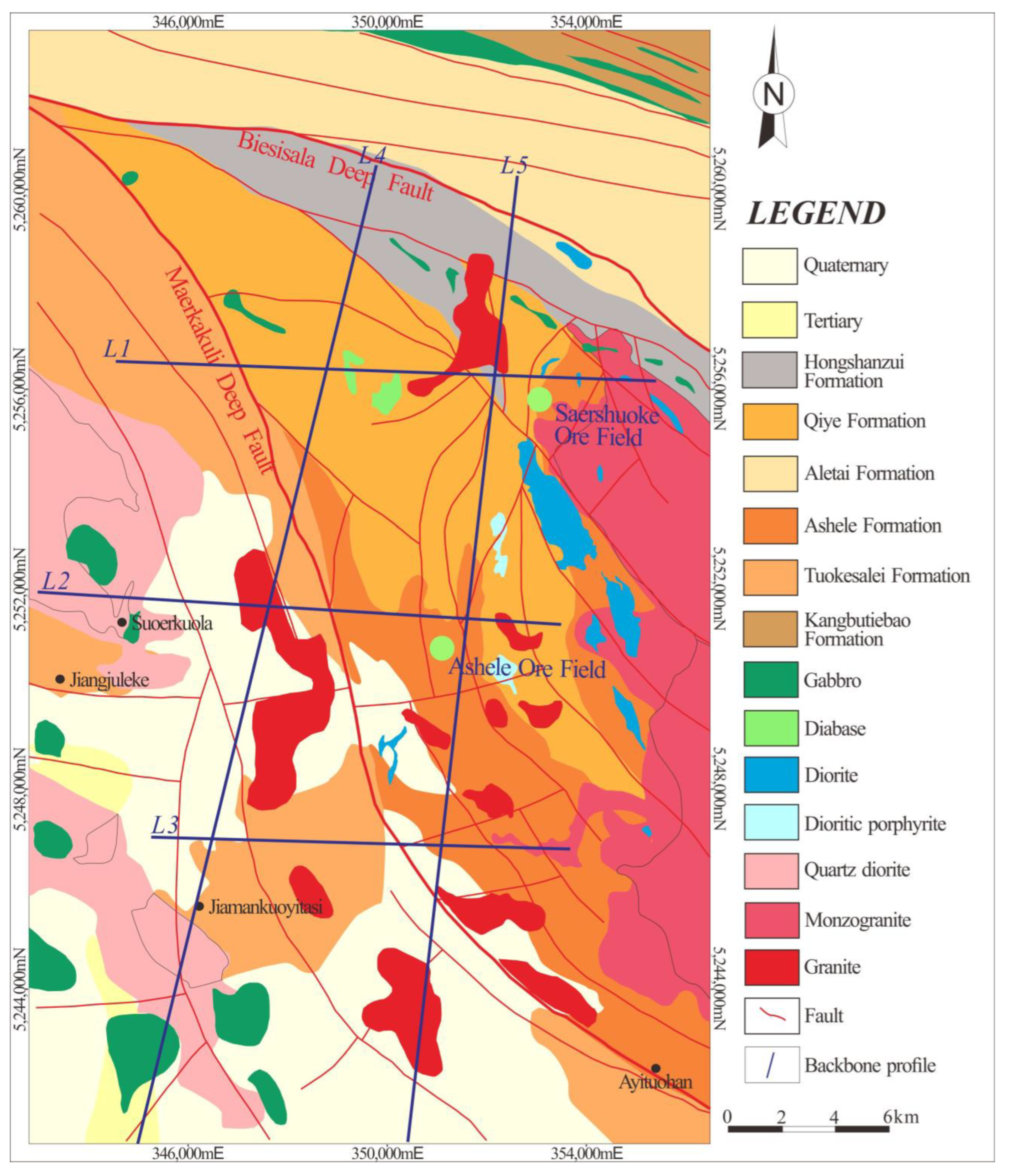
2. Geological Setting

The study area is geotectonically located at the junction of the Ashele island arc tectonic area (a secondary tectonic unit of the late Paleozoic arc-basin system in the South Altay orogenic belt of the Siberia Plate) and the Habahe late Paleozoic forearc basin (Figure 1). The magmatic activity is strong in the study area, and volcanic rocks, subvolcanic rocks, and intrusive rocks are developed there. The volcanic rocks, which were formed from the Early Devonian to the Early Carboniferous, are distributed in the Ashele island arc structure. The intrusive rocks are mostly Hercynian intermediate and felsic plutons, with locally distributed intermediate and mafic plutons, and these rocks are distributed on the east and west sides of the Maerkakuli fault, mainly represented by the Habahe pluton in the east and the Bieliezekehe pluton group in the west [17,18,19,20,21].
The strata in the study area mainly include the Quaternary, Tertiary, and Carboniferous Hongshanzui Formation; the Upper Devonian Qiye Formation; the Middle Devonian Ashele Formation; the Middle Devonian Altay Formation; the Lower-Middle Devonian Tuokesalei Formation; and the Lower Devonian Kangbutiebao Formation. The lower part of the Kangbutiebao Formation is dominated by sedimentary rocks, and its upper part is dominated by volcanic lava and tuff, with different lithologies such as schist, quartz feldspar sandstone, siltstone, felsic tuff, and carbonate rock. The Kangbutiebao Formation is in fault contact with the overlying Altay Formation. The main lithologies of the Tuokesalei Formation are graywacke, siltstone, phyllite, crystalline limestone, and siliceous rock. The Tuokesalei Formation is in fault contact with the Ashele Formation, Qiye Formation, and Hongshanzui Formation. The main lithologies of the Altay Formation are metamorphic fine sandstone, metamorphic siltstone, two-mica quartz schist, and sericite-quartz schist. The Altay Formation is in fault contact with the Hongshanzui Formation. The main lithologies of the Ashele Formation are crystal-vitric tuff, breccia-bearing tuff, and tuff, and it is in angular unconformable contact with the overlying Qiye Formation. The main lithologies of the Qiye Formation are rhyolite, andesite, basalt, and their corresponding pyroclastic rocks, and it is in angular unconformable contact with the overlying Hongshanzui Formation and the underlying Ashele Formation. The main lithologies of the Hongshanzui Formation are metabasalt, metabasaltic andesite, meta-andesite, meta-dacite, and their corresponding pyroclastic rocks. The Hongshanzui Formation is in fault contact with the Altay Formation in the northeast and in angular unconformable contact with the Qiye Formation in the southwest [22,23]. Fold and fault structures are developed in the area. The fold structures are generally northwest-trending, showing strong cleavage and linear tight folds, and secondary folds are developed. The fault structures are also generally northwest-trending, and the main faults include the Maerkakuli fault and the Biesisala fault.
Typical deposits in the study area are the Ashele copper–zinc deposit and the Saershuoke gold–copper polymetallic deposit. The Ashele copper–zinc deposit is tectonically located in the southwestern part of the Altay orogenic belt and east of the Maerkakuli fault. Its proven ore bodies are mainly located in the inverted syncline, and the Ashele Formation is the main ore-bearing horizon of the deposit. The Saershuoke gold–copper polymetallic deposit is located approximately 5.6 km northeast of the Ashele copper–zinc deposit. Its ore bodies mainly occur in the rhyolite porphyry of the Ashele Formation and are obviously controlled by horizons. The shallow gold–copper ore bodies mainly occur in the form of veins and network veins, and the deep lead–zinc ore bodies are mainly stratiform-like. The ores are mainly massive, densely disseminated, and sparsely disseminated [17,24,25].

3. Three-Dimensional Modeling Method

The basic idea of this method is to establish a sparse backbone profile using the geological and geophysical data to control the overall structural framework of the study area and then construct a 3D geological model based on the backbone profile through interpolation. Next, the geological model is converted to a physical property model for 3D gravity and magnetic inversion, and the model is modified by gradually adding an auxiliary section at any position until the inversion results are satisfactory. Each auxiliary section can be a plane or a profile with any inclination, strike, and size. Figure 2 shows the overall process of the method. The modeling process mainly includes six steps: data sorting, information processing and interpretation, key geological profile construction, 3D geological model construction, 3D constrained inversion, and model visualization.
Data sorting: Relevant data mainly include geological, borehole, physical property, geophysical, and geochemical data. The collected information is divided into two categories according to the requirements: constraint information and basic information. Constraint information refers to the information that can indirectly constrain the shape of the model, mainly including geophysical data, geochemical data, borehole data, etc. Basic information refers to the indispensable information that always participates in the inversion modeling process. It mainly includes geological and physical properties.
Information processing and interpretation: This mainly refers to the mining, augmenting, and extracting of effective information from constrained information. For geophysical data (gravity, magnetic, and electric), multi-scale edge detection and grid inversion are performed to extract effective information about geological units (such as faults, plutons, and strata) based on conventional gridding, filtering, and potential field separation.
Construction of the backbone geological profile: The positions of the profiles are planned with the goal of controlling the overall tectonic framework of the study area. The interpretation of the constraint information is used to infer and plot the profile to reflect the spatial distribution of strata, faults, plutons, and ore bodies in the area that the profile passes through. After the preliminary construction of the profile is completed, the profile shape is vectorized and imported into inversion software. The mature 2.5D gravity and magnetic inversion modeling technology is used to correct the profile to determine the final shape of the backbone geological profile.
Construction of the 3D geological model: The inverted and corrected backbone geological profile, the measured and interpreted structural information, and the surface geological map are imported into the 3D space after determining the scope of the modeling space and adding the topographic data. Then, visualization and interpolation technologies are used to build a 3D geological model. At this time, the model mainly depicts the overall geological structural framework of the study area, and the details of the model are not well matched with the actual geological conditions. In the later stage, multiple constrained inversions are carried out to continuously correct and improve the geological model.
Three-dimensional constrained inversion: Using the gravity and magnetic data after potential field separation as the basic inversion data, the 3D geological model is converted into a physical property model according to our physical property analysis. The physical property model is then subjected to constrained inversion. The boundaries of the geological bodies are known conditions that cannot be easily changed. During inversion, the physical properties of the geological units are adjusted first, and then auxiliary sections are added one by one to modify the boundaries of the geological bodies to fit the measured data. Eventually, the 3D model matches not only the geological understanding but also the gravity and magnetic data.
Model visualization: The built model is imported into a visualization platform, such as Encom PA or Voxel. The spatial structures of geological bodies are analyzed in depth to extract the geological information for predicting deep mineralization or for analyzing the spatial relationship between mineralization-related geological bodies to establish metallogenic models. The model can also be used for mine design, reserve calculation, and deep and peripheral ore body prediction [7,26,27,28].

4. Interpretation of the Data

4.1. Arrangement and Analysis of the Physical Property Data

The analysis of the physical property data shows that the strata in the ore concentration area are generally less dense than the intrusive rocks in the study area (Table 1), which is related to the main lithologies (i.e., normal sedimentary rocks and intermediate–felsic volcanic rocks) of each stratum and the destructive tectonic activities and frequent magmatic hydrothermal activities in different periods. Quartz diorite (on one side of the Habahe pluton), skarn, diorite, gabbro, and diorite porphyrite have the highest densities among the rocks in the study area, with narrow lithological distribution ranges, mostly in the form of veins and clusters, which often cause high-value gravity anomalies with high amplitudes and steep gradients in this area. Quartz diorite (southwest of the Maerkakuli fault) and basaltic andesite have high densities. Monzogranite has medium densities. The mafic rocks (gabbro, etc.) in the area have obviously different densities than the surrounding rock, and the high-gravity anomalies or the weak-gravity anomalies in the periphery of high-gravity anomalies are mostly buried or semi-buried basic rock mass (Table 1).
Magnetic analysis shows that the marine intermediate–felsic volcanic rocks in the Ashele Formation have weak magnetism, while the Upper Devonian Qiye Formation has relatively strong magnetism and uneven magnetic changes. The intermediate–mafic pyroclastic rocks and volcanic lava on the eastern side of the Maerkakuli fault have strong magnetism, while the other areas are relatively weak. These characteristics of magnetism reflect the relative enrichment of magnetic minerals in the eastern region due to the influence of the Habahe plagioclase granite pluton. Normal sedimentary rocks, intermediate–felsic–mafic pyroclastic rocks, and volcanic lava are generally nonmagnetic, and a small portion of them are inhomogeneously and weakly magnetic. Some breccias and breccia lava are moderately magnetic. Intermediate–mafic subvolcanic rocks are generally weakly magnetic, and some plutons are moderately magnetic. Skarn and some quartz diorites are moderately magnetic, while gabbros are strongly magnetic and can cause obvious magnetic anomalies.
Notably, petrophysical properties vary with depth. In the 3D inversion of potential field data, it is crucial to comprehensively study and analyze the variation laws of the main petrophysical properties with burial depth, which mainly depend on the physical property analysis of borehole samples. Although such information is limited in this study area, the available data still provide important basic data support for modeling. In addition, affected by different geological conditions and tectonic activities, the physical properties of the same lithology differ between regions. For example, the quartz diorite near the Habahe pluton and the quartz diorite in the southwest of the survey area have certain differences in density and magnetic susceptibility, so the two should be distinguished during inversion and modeling.

4.2. Geophysical Information Processing and Interpretation

We next collected and sorted out the previous geological, borehole, geophysical, and geochemical exploration data in the ore concentration area [15,16,17,18,19,20,21,22,23,24,25]; carried out gravity, magnetic and magnetotelluric profile survey in the area; conducted gridding, potential field separation, information enhancement, and other processing; and comprehensively analyzed the study area based on the processing results, the physical property analysis, geological data, and borehole information.

4.2.1. Information Processing

1.
Gravity and magnetic data
We used a surveying grid with a line spacing of 500 m and point spacing of 100 m, with a CG-5 gravimeter gravity acquisition instrument and a Trimble R8 dual frequency differential GPS positioning instrument to acquire gravity data, and the simple Bouguer data gridded to 500 m. The magnetic data were acquired with a grid spacing of 250 m × 50 m and have been gridded to 100 m × 100 m, and we used a reduction-to-the-pole (RTP) filter with a magnetic inclination of 69.1°, declination of 4.5°, and the RTP magnetic anomaly shown in Figure 3C.
Potential field separation is an important step in data processing [29,30,31]. First, a variety of potential field separation methods are used to process the gravity and magnetic data, and then appropriate separation results are selected for basic statistical analysis through comparisons. The comparisons mainly include two aspects. One is the comparison between the processing results of different methods (if two or more methods generate similar processing results, the applied processing methods are considered to be reasonable); the other is the comparison between the processing results and the known actual geological conditions (if the processing results of a method are in accordance with exposed geological bodies or the spatial positions of the proven geological bodies, the processing method is reasonable enough).
In this study, after smoothing, gridding, and reducing to the pole (this method is only applied to magnetic data) the gravity and magnetic data, the potential field data are separated by means of upward continuation, moving average, matched filtering, and trend analysis. The residual anomalies obtained by the moving average method are selected as the basic data for constrained inversion and analysis (Figure 3B,D).
The Bouguer gravity anomalies in the area are mostly northwest-trending (Figure 3A). These anomalies are overall high in the southwest and low in the northeast with the Maerkakuli fault as the dividing line, which objectively reflects two regional geological structures: the Ashele island arc structure east of the fault and the late Paleozoic Habahe forearc basin west of the fault. Among the residual gravity anomalies, the relatively high anomalies are northwest–southeast-trending and are mostly distributed in the western and central parts of the study area, showing various shapes, mostly elliptical, banded, and moniliform, with local annular features (I~IV in Figure 3B). These relatively high anomalies are related to the widespread distribution of Carboniferous and Permian intermediate and mafic volcanic rocks and intrusive rocks in this area. The high-gravity anomalies in the Quaternary coverage in the southwestern ore concentration area are characterized by small amplitude, small scale, and gentle variation, and the low-gravity anomalies mixed in among the high-gravity anomalies are mostly distributed in bands. Some of the planar anomalies coincide with the magnetic anomalies and, we infer, are buried gabbro plutons. Low-gravity anomalies are often distributed in bands and ellipses along the edges of fault structures and are inferred to be the comprehensive response of plutons and fault structures, and the distribution of the plutons along the fault structures indicates that magmatic activity has a close relationship with the fault structures in the study area. In addition, the fault structures have a strong destructive effect on the early strata, as confirmed by the differently shaped distributions of low-gravity anomalies in the Qiye and Ashele Formations.
Magnetic anomalies have various shapes, mostly linear, moniliform, or elliptical, with variable strikes and poor continuity. High magnetic anomalies are mainly distributed near the east, west, and north boundaries of the survey area (Figure 3C,D). According to the analysis of surface exposure and physical property data, we preliminarily conclude that the northern high magnetic anomaly was caused by exposed and buried banded diabase. The western magnetic anomalies are distributed in northwest-trending and north–south-trending bands. The northwest-trending anomalies are inferred to be the responses of quartz diorite, and the north–south-trending anomalies are inferred to be responses to the magnetic enhancement of the volcanic strata caused by the relatively strong hydrothermal activity at the edges of the plutons. The eastern magnetic anomalies are caused by diorite, quartz diorite, and buried magnetic bodies. The beaded high-value magnetic anomalies in the Kangbutiebao Formation, in the northeast corner of the area, are inferred to be caused by exposed and hidden banded diabase. The part of the study area corresponding to the Altay Formation shows weak, low-gradient magnetic anomalies. The northwest-trending banded magnetic anomalies in the east-central part of the survey area are between 100 and 500 nT, and they are inferred to be the responses of the sporadic buried gabbro. The magnetic anomaly in the southwest corner is composed of multiple planar magnetic anomalies, showing a complex shape. It is likely a response of gabbro, according to the borehole results in this area.
2.
Magnetotelluric profile data
Five backbone profiles were planned in this study, including two nearly north–south profiles and three nearly east–west profiles (L1–L5 in Figure 4). The profiles were measured by the magnetotelluric method and processed to obtain the resistivity distribution results, which served as a basis for comprehensive profile interpretation and analysis and model profile modification.
The MTU-5A Satellite-Synchronized Data Acquisition System was used for data acquisition with a frequency range of 0.001 Hz–32 0 Hz. The measurement time of each station is greater than 12 h, and the distance between the stations is about 200 m. The length of Line 1 is 10.60 km, and the azimuth angle is 92°NE. The length of Line 2 is 10.55 km, and the azimuth angle is 93°NE. The length of Line 3 is 8.60 km, and the azimuth angle is 92°NE. Line 4 is approximately 20.20 km long, and the azimuth angle is 14°NE. Line 5 is approximately 19.60 km long, and the azimuth angle is 6°NE. The professional processing software named SSMT-2000 (2.1.5.0) is used to carry out the processing of the collected data, and the obtained resistivity data have been gridded to 200 × 200 m.

4.2.2. Information Interpretation

3.
Interpretation of gravity and magnetic data
The potential field data are interpreted in two aspects (fault structure interpretation and rock mass interpretation) based on the statistical results of physical properties, the sparse constrained inversion results of physical properties, and geological and borehole data.
Fault structure interpretation: Fault structures in the area are characterized by multistage activity and are usually composed of multiple faults. The rigid rocks and fine-grained clastic rocks in the fault zone are highly fragmented and argillized, respectively, which manifests as an obvious combination of low-gravity and low-resistivity anomalies in the gravity gradient zone. The characteristics of magnetic anomalies differ between geological conditions because fault structures are the most important migration channels and precipitation sites of hydrothermal fluids. In the presence of late hydrothermal fluid activities along the deep fault structures or magmatic–hydrothermal activities with different properties, the magnetic anomalies tend to show complex characteristics. In this study, 34 faults were identified by combining the processing results of gravity, magnetic, and magnetoelectric data with geological, borehole, and other information. Then, the lengths, trends, and dip angles of these faults were determined, digitized, and edited into 3D space (Figure 5). As shown by the 3D model, the fault structure in the Ashele Basin is developed with complex morphology, which indicates that there are more geological structural activities in this area. The spatial relationship between the ore bodies and the faults shows that the areas where faults develop in the study area are more likely to be favorable metallogenic areas.
Intrusive rocks interpretation: The intermediate intrusive rocks in the study area are diorites, which can be roughly classified into three types according to their material composition: relatively mafic pyroxene diorite, intermediate diorite, and relatively felsic quartz diorite (granite diorite). The first two types are mostly characterized by the combination of high-gravity anomalies, medium–high magnetic anomalies, and high-resistivity anomalies, and the third type is mostly characterized by the combination of low-gravity anomalies, weak or no magnetic anomalies, and high-resistivity anomalies. According to published statistics on various physical properties, the combination of high magnetic anomalies, high-gravity anomalies, and high-resistivity anomalies is a typical sign for the presence of mafic–ultramafic plutons. In the actual analytical process, the geological situation is often much more complicated, so the identification and interpretation of rock masses need to be based on a comprehensive analysis of the geological background and geological processes. A total of 26 rocks in the study area were identified, including 12 intermediate–acidic intrusive rocks, 4 intermediate intrusive rocks, and 10 mafic intrusive rocks. The intermediate–acidic intrusive rocks are mainly concentrated in the peripheries of the Maerkakuli fault and the Biesisala fault zone in the middle of the study area. This type of rock is usually deep and relatively large. The four intermediate rocks include two diorite rocks located in the southern part of the survey area and two quartz diorite rocks located at the western boundary of the study area. The 10 mafic rocks include 8 gabbro rocks and 2 diabase rocks (Figure 4).
4.
Interpretation of the magnetotelluric profiles
Five backbone profiles were collected by magnetotelluric survey at the planned positions. Line 2, the survey profile passing through the Ashele mining area in the middle of the Ashele Basin, is taken as an example of how to interpret the magnetotelluric profiles. The interpretation is briefly described below (Figure 6).
Line 2 is approximately 10.55 km long. The profile starts from the Donggele pluton in the west of the basin, crosses the Maerkakuli ductile shear zone eastward, and enters the north of Ashele Village and then passes through the Ashele copper–zinc mining area and enters the volcanic rock area of the Qiye Formation east of the mining area. The characteristics of shallow high–low resistivity anomalies indicate that there are steep east-dipping fault structures in the shallow part of the basin, which are coincident with the known locations of faults determined based on the surface geological survey and gravity and magnetic field anomalies, among which the Maerkakuli fault is the most prominent. The deep position in the west of the basin presents an asymmetrical basin-shaped low-resistivity anomaly dipping eastward. The basement of the eastern segment shows a high-resistivity uplift with the western boundary uplifted to the east, and the surface is composed of exposed volcanic rocks of the Ashele Formation. The low-resistivity anomaly extends up to approximately 1600 m deep. The northern segment of the main ore body of the Ashele copper mine is located on the east side of the basin-shaped low-resistivity anomaly. The copper ore occurrences in northern Ashele Village are exposed on the west side of the basin-shaped anomaly, and the known mineralized bodies in the deep part of the ore prospecting target are verified by boreholes. The shallow high resistivity corresponds to the volcanic rocks of the Qiye Formation on the surface. The other four backbone profiles are also analyzed in detail one by one.

5. Model Building

5.1. Construction of the Backbone Profiles

Taking Line 2 as an example, we briefly describe the construction process of the backbone profiles. First, the initial 2D geological profile is inferred and drawn. The distribution of surface geological units is constrained by the surface geological map, and the extension and distribution of deep geological bodies are constrained by borehole data and magnetotelluric profiles. The interpretation of the magnetotelluric profile provides basic information for the initial 2D geological profile, such as the shapes of the quartz diorite and gabbro in the west of the profile, the shapes of granite in the middle of the profile, the basement depth of the Ashele Basin, and the location of some faults, which are important foundations for establishing the initial geological profile.
Then, based on the initial geological profile, a 2.5D model is established, and forward and inversion calculations are performed using Encom’s ModelVision Pro™. Based on the residual gravity and magnetic anomalies, the model and physical parameters are continuously modified by man–machine interaction until a reasonable geological model and a satisfactory fitting effect are obtained (Figure 7). The other four backbone profiles are constructed by the same method.

5.2. Construction of the Three-Dimensional Geological Model

The modeling space is a north–south-trending cuboid, with an east–west length of 13.7 km, a north–south length of 22.3 km, and an altitude of 2000 m to −3000 m. The modeling involves 18 geological units, and the chronological order of the geological units and the contact relationship between them are determined at the same time.
The five inverted and corrected backbone geological profiles, surface geological maps, and topographic data are input into the modeling space, and visualization and interpolation techniques are used to connect the boundaries of the same geological unit to establish a 3D geological model (Use GeoModeller™ 4.2.0).

5.3. Three-Dimensional Constrained Inversion

The obtained 3D geological model is converted into a physical property model by introducing physical parameters. Then, the physical property model is meshed to grid cells of 200 m × 200 m × 50 m before 3D gravity and magnetic inversion. The gravity inversion is the focus of inversion, the magnetic inversion being subsidiary.
The physical property parameter settings refer to the physical property variation ranges determined by the physical property analysis and are input into the inversion software in the form of means and mean square errors as important constraints in the physical property inversion.
When the data are input into the modeling software, all kinds of data are divided into four categories (observed, inferred, interpreted, and unspecified) according to the data sources, and constraint information such as borehole, surface geological maps, and profile are divided into the same category (observed). In the inversion process, this category of data is set to remain the boundary position unchanged using software (GeoModeller™ 4.2.0). In all, the boundaries of the geological bodies involved in the surface geological maps, profiles, boreholes, etc., serve as constraints and remain unchanged during the inversion process.
After the inversion, the measured gravity and magnetic data are compared with the data simulated by forward modeling, and the model is corrected in the areas with a large shape difference (fit difference) between the two. First, the rationality of the physical parameters is checked. For example, we checked whether there were special geological conditions in the mismatched areas, such as changes in physical properties (alteration, silicification, etc.) of the same lithology due to different geological environments. If changes in physical properties are not the cause of a mismatch, the boundaries of the corresponding geological unit are corrected by gradually adding auxiliary sections to reduce the fitting error of 3D inversion, and the model is revised repeatedly until the measured data match well with the data simulated by forward modeling (Figure 8 and Figure 9).
The final fitting error for the gravity data is 0.3919 mGal, indicating satisfactory overall fitting. The large fitting errors are concentrated in the southeast corner of the survey area. The fitting error for the magnetic data is 90.94 nT, and their relatively large errors are located at the edge of the southwest corner of the survey area.
A total of 10 auxiliary sections were constructed in this study, including four planes and six profiles. Auxiliary sections are mostly used to finely depict the shapes of the plutons, and the depths of the plutons are determined based on the borehole information or the analysis results of the backbone profiles. The specific functions of the auxiliary sections include (1) facilitating the backbone profiles to control the spatial shapes of the geological bodies; (2) supplementing the blanks caused by sparse information in some areas; and (3) facilitating the control of the shapes of the geological structures in peripheral areas and correcting the edge effect caused by the basic data.

6. Results and Discussion

6.1. Structural Characteristics of Three-Dimensional Model

Using visualization software, the final 3D geological–geophysical model of the Ashele ore concentration area (Figure 10) is presented from different perspectives. The 3D model is observed and analyzed from different angles and distances, and each geological unit is briefly described as follows (Figure 11):
Quaternary and Tertiary strata: The Quaternary and Tertiary strata in the study area are mainly concentrated in the southwest of the survey area, with thicknesses generally ≤100 m.
Hongshanzui Formation: The Hongshanzui Formation is generally northwest–southeast-trending, showing a shuttle-shaped distribution. The formation gradually becomes thinner from the southeast to the northwest and disappears at the northwest corner of the study area. The formation is in fault contact with the Qiye Formation and the Altay Formation.
Qiye Formation: The Qiye Formation is generally northwest–southeast-trending, showing a triangular distribution. Its southern segment overlies the Ashele Formation. The thickness of the Qiye Formation varies greatly but is overall larger in the east than in the west and larger in the north than in the south. There are local fault structures in the Ashele Formation.
Altay Formation: The Altay Formation is nearly east–west-trending, showing an elongated distribution. Its thickness usually exceeds 2000 m and is relatively larger in the east but otherwise does not have much spatial variation.
Ashele Formation: The Ashele Formation shows a north–south-trending planar distribution with an inverted-triangle shape. The southwest side of the formation is bounded by the Maerkakuli fault and is in fault contact with the Tuokesalei Formation. The east side of the formation is bounded by the Habahe pluton and has a tendency to extend to the outside of the area in its deep part. The central part of the northern segment of the formation (north of Ashele) extends slightly to the north, while the east and west sides of the northern segment of the formation both extend to the northwest and northeast to a certain extent. The thickness of the south segment of the formation generally exceeds 2000 m, which is thicker than the rest of the formation. The model shows that there is an obvious W-shaped fold structure in the Ashele Formation. The Ashele mining area and the Saershuoke mining area are both located on the anticline of the large fold structure. There are local fault structures in the Ashele Formation, most of which are northwest-trending. Many intermediate plutons are exposed on the surface, and there are many buried intermediate–felsic plutons in the deep part.
Tuokesalei Formation: The Tuokesalei Formation is bounded by the Maerkakuli fault in the northeast, and most of the formation is covered by the Quaternary and Tertiary series. This formation has relatively high and uniform thickness, more than 3000 m in the study area. The formation contains many buried intermediate–felsic plutons and mafic plutons but only a few fault structures (mainly the Maerkakuli fault and its secondary structures), which are mostly northwest-trending.
Kangbutiebao Formation: The northwest-trending Kangbutiebao Formation is in the northeast corner of the study area, showing an elongated distribution. The maximum thickness of the formation is approximately 2000 m, and there are local diabase intrusions in the formation.
Basement: The basement is overall higher in the north than in the south and higher in the west than in the east. The basement has an obvious uplift in the Ashele Basin. The maximum thickness of the basement in the modeling area is approximately 1000 m, and the southwest segment of the basement extends to greater depths.
Plutons: The visualization results of the 3D model clearly indicate the distribution shape, depth, and scale of the plutons. The plutons on the east and west sides of the study area are the extensions of the Habahe and Donggele plutons into the study area. These two plutons are large. The maximum depth of the Donggele pluton in the area exceeds 3500 m, and the maximum depth of the Habahe pluton exceeds 2500 m. There are many buried and semi-buried plutons in the area, including gabbro plutons, diabase plutons, felsic granite plutons, monzonitic granite plutons, intermediate diorite plutons, quartz diorite plutons, etc. The gabbro plutons are mainly located at the western edge of the survey area and south of Jiamankuoyitasi on the southwest side of the survey area. The gabbro plutons are relatively large. Most of them are columnar and moniliform intrusions in the strata, some of them are exposed to the surface, and most of them are buried plutons with relatively shallow burial depth (<1000 m, mostly near the surface). The diabase plutons are mostly in the northeast corner of the study area, and they are northwest-trending vein-like intrusions into the Kangbutiebao Formation, with a maximum depth of approximately 200 m in the study area. The felsic granite plutons are mostly located near the Maerkakuli fault, with different scales (the felsic granite plutons in the deep part are relatively larger) and various shapes (mostly columnar, stalagmitic, moniliform, strip-shaped, or saddle-shaped intrusions in the strata). The intermediate diorite plutons are mostly located in the east and north of the survey area and are mostly exposed to the surface, showing a banded distribution, and they are generally less than 500 m deep.

6.2. Enlightenment about Ore Prospecting

There are various types of mineralization in the Ashele ore concentration area, including layered copper–zinc mineralization and barite mineralization formed by jet deposition, vein-like copper (zinc) mineralization, and copper–lead–zinc–silver mineralization formed in the supply channel, vein-like gold–copper–lead–zinc mineralization and copper mineralization in subvolcanic rocks, copper mineralization in the contact zone of subvolcanic rocks, and copper mineralization in faults or fissures. These mineralizations are found in the Devonian Ashele Formation, which is the main ore-bearing horizon, and the deep distribution pattern of the formation can be an important guide for ore prospecting. The 3D model indicates that the Ashele Formation on the north side of the Ashele mining area mainly extends to the deep part, so the Ashele copper–zinc ore body likely continues northward to the deep part. In the area where the Saershuoke polymetallic deposit is located, its ore-forming strata of the Ashele Formation mainly continue eastward in the deep part, so its prospecting direction should also be eastward. These all suggest directions for further prospecting work.
Based on the 3D model, this paper analyzes the spatial distribution of strata, plutons, faults, etc., and delineates three deep metallogenic prospective areas, namely, the Chuangayi prospective area, the Ashele northern prospective area, and the Saershuoke eastern prospective area, based on the results of typical ore deposits (Figure 12).

6.3. Discussion

The 3D geological–geophysical modeling technology can trace the deep distribution of metallogenic geological bodies and visualize the ore-controlling structures to achieve ore prospecting prediction, but the proposed method still has limitations. For example, the accuracy of magnetic inversion in this study needs to be improved. The main reason is that there have been multiple episodes of strong tectonic activity in the study area, which makes the magnetic properties of the same type of stratigraphic unit differ greatly between regions. Therefore, it is necessary to conduct a more detailed survey of the physical properties with more modeling units and greater meshing density to improve the inversion fitting accuracy, but this also means increased workload and computation time. The research objectives and other factors, such as the scale and accuracy of the basic data, should be comprehensively considered to formulate a reasonable end-of-inversion accuracy.

7. Conclusions

This study has established a 3D geological–geophysical model of the Ashele ore concentration area within a depth of 5000 m, realized the “transparency” of the Ashele ore concentration area for the first time, and obtained the 3D spatial distributions of 9 formations, 10 types of plutons, and 34 faults, laying the foundation for geological research and prospecting work.
The results of this study will help researchers to have a clearer understanding of the deep geological structure and the 3D distribution of faults and plutons in the study area, which will improve the understanding of the basic geological conditions and provide support for deep prospecting work. At the same time, combined with the geological data of typical deposits, three metallogenic prospect areas are predicted, which points out the direction for the ore prospecting in Ashele. This study can provide a reference for prospecting work in similar ore concentration areas and overburdened areas with sparse data.
The modeling method and process proposed in this study have good applicability to the construction of 3D models of large ore concentration areas with relatively sparse data and complex geological structures. Gradually adding the auxiliary sections can modify the model more reasonably and efficiently to fit the measured anomalies, thus effectively reducing the time taken to establish unnecessary profiles to reduce modeling time. The use of auxiliary sections with arbitrary directions, dip angles, depths, and lengths can make full use of known information and can consider changes in geological units in different directions to more accurately reflect the actual geological conditions.

Author Contributions

Conceptualization, G.M. and G.Q.; formal analysis, G.Q., G.M. and J.Y.; methodology, G.Q. and G.M.; investigation, G.Q., H.T. and R.X.; visualization, G.Q. and H.T.; writing—original draft, G.Q.; writing—review and editing, G.Q., G.M. and J.Y.; project administration, G.M. and G.Q. All authors have read and agreed to the published version of the manuscript.

Funding

This research was funded by the Deep Geological Survey Program of China (DD20230008, DD20221643), and the National Key R&D Plan Program of China (2018YFC0604002).

Data Availability Statement

Data sharing is not applicable to this article.

Acknowledgments

The authors are grateful for the constructive comments by the anonymous reviewers.

Conflicts of Interest

The authors declare no conflict of interest.

References

  1. Tonini, A.; Guastaldi, E.; Massa, G.; Conti, P. 3D geo-mapping based on surface data for preliminary study of underground works: A case study in Val Topina (Central Italy). Eng. Geol. 2008, 99, 61–69. [Google Scholar] [CrossRef]
  2. Zanchi, A.; Donatis, M.D.; Gibbs, A.; Mallet, J.L. Imaging geology in 3D Preface. Comput. Geosci. 2009, 35, 1–3. [Google Scholar] [CrossRef]
  3. Akiska, S.; Sayili, I.S.; Demirela, G. Three-dimensional subsurface modeling of mineralization: A case study from the Handeresi Pb-Zn-Cu deposit. Turk. J. Earth Sci. 2013, 22, 574–587. [Google Scholar] [CrossRef]
  4. Collon, P.; Steckiewicz-Laurent, W.; Pellerin, J.; Laurent, G.; Caumon, G.; Reichart, G.; Vaute, L. 3D geomodelling combining implicit surfaces and Voronoi-based remeshing: A case study in the Lorraine Coal Basin (France). Comput. Geosci. 2015, 77, 29–43. [Google Scholar] [CrossRef] [Green Version]
  5. Wang, G.W.; Zhang, S.T.; Yan, C.H.; Song, Y.W.; Sun, Y.; Xu, F.M. Mineral potential targeting and resource assessment based on 3D geological modeling in Luanchuan region, China. Comput. Geosci. 2011, 37, 1976–1988. [Google Scholar] [CrossRef]
  6. Williams, H.A.; Betts, P.G.; Ailleres, L. Constrained 3D modeling of the Mesoproterozoic Benagerie Volcanics Australia. Phys. Earth Planet. Inter. 2009, 173, 233–253. [Google Scholar] [CrossRef]
  7. Schetselaar, E.; Ames, D.; Grunsky, E. Integrated 3D Geological Modeling to Gain Insight in the Effects of Hydrothermal Alteration on Post-Ore Deformation Style and Strain Localization in the Flin Flon Volcanogenic Massive Sulfide Ore System. Minerals 2018, 8, 3. [Google Scholar] [CrossRef] [Green Version]
  8. Olierook, H.K.; Scalzo, R.; Kohn, D.; Chandra, R.; Farahbakhsh, E.; Clark, C.; Reddy, S.M.; Müller, R.D. Bayesian geological and geophysical data fusion for the construction and uncertainty quantification of 3D geological models. Geosci. Front. 2021, 12, 479–493. [Google Scholar] [CrossRef]
  9. Lu, Q.T.; Qi, G.; Yan, J.Y. 3D geologic model of Shizishan ore field constrained by gravity and magnetic interactive modeling: A case history. Geophysics 2013, 78, B25–B35. [Google Scholar] [CrossRef]
  10. Qi, G.; Lv, Q.T.; Yan, J.Y.; Wu, M.A.; Deng, Z.; Guo, D.; Shao, L.S.; Chen, Y.J.; Liang, F.; Zhang, S. 3D geological modeling of Luzong ore district based on priori Information constrained. Acta Geol. Sin. 2014, 88, 466–477. [Google Scholar]
  11. Yan, J.Y.; Lv, Q.T.; Qi, G.; Fu, G.M.; Zhang, K.; Lan, X.Y.; Guo, X.; Wei, J.; Luo, F.; Wang, H.; et al. A 3D geological model constrained by gravity and magnetic inversion and its exploration implications for the world-class Zhuxi tungsten deposit, South China. Acta Geol. Sin. 2020, 94, 1940–1959. [Google Scholar] [CrossRef]
  12. Xu, Y.; Liu, Y.; Wu, H. 3D Geological Modeling of Deeply Buried Tuff Orebody Based on Parallel Sections and Gradual Deformation Method. Minerals 2019, 9, 230. [Google Scholar] [CrossRef] [Green Version]
  13. Arias, M.; Nuñez, P.; Arias, D.; Gumiel, P.; Castañón, C.; Fuertes-Blanco, J.; Martin-Izard, A. 3D Geological Model of the Touro Cu Deposit, A World-Class Mafic-Siliciclastic VMS Deposit in the NW of the Iberian Peninsula. Minerals 2021, 11, 85. [Google Scholar] [CrossRef]
  14. Zhang, X.L.; Wu, C.L.; Zhou, Q.; Weng, Z.P.; Yuan, L.J.; Zhu, F.K.; Li, Z.L.; Zhang, Z.T.; Yang, B.N.; Zhao, Y.T. Multi-Scale 3D Modeling and Visualization of Super Large Manganese Ore Gathering Area in Guizhou China. Earth Sci. 2020, 45, 634–644. [Google Scholar] [CrossRef]
  15. Meng, G.X.; Tang, H.J.; Liu, H.Y.; Qin, J.H.; Wu, X.G.; Li, C.W. Devonian igneous rocks and tectono-magmatic evolution in the Ashele basin, Xinjiang. Acta Geol. Sin. 2022, 96, 445–464. [Google Scholar]
  16. Yang, F.Q.; Wu, Y.F.; Yang, J.J.; Zheng, J.H. Metallogenetic Model for VMS Type Polymetallic Copper Deposits in the Ashele Ore Dense District of Altay, Xinjiang. Geotecton. Metallog. 2016, 40, 701–715. [Google Scholar]
  17. Yang, F.Q.; Liu, F.; Li, Q. Geological characteristics and metallogenesis of the Saershuoke polymetallic deposit in Altay, Xinjiang. Acta Petrol. Sin. 2015, 31, 2366–2382. [Google Scholar]
  18. Lin, Z.F.; Yuan, C.; Zhang, Y.Y.; Sun, M.; Long, X.P.; Wang, X.; Huang, Z. Triassic depleted lithospheric mantle underneath the Paleozoic Chinese Altai orogen: Evidence from MORB-like basalts. J. Asian Earth Sci. 2019, 185, 104021. [Google Scholar] [CrossRef]
  19. Zheng, C.J.; Liu, P.F.; Luo, X.R.; Wen, M.L.; Huang, W.B.; Liu, G.; Wu, X.G.; Qiu, W.; Chen, Z.S.; Xiao, H.; et al. Rock Geochemical Data Mining and Weak Geochemical Anomaly Identification—A Case Study of the Ashele Copper-Zinc Deposit, Xinjiang, NW China. Geotecton. Metallog. 2022, 46, 86–101. [Google Scholar]
  20. Zhao, C.C.; Tang, S.H.; Qin, M.; Guo, X.W.; Jiao, W.Y.; Liu, C. Fractal characteristics of spatiotemporal distribution and activity prediction based on mine earthquake—Taking the Ashele copper mine in Xinjiang as an example. Chin. J. Rock Mech. Eng. 2019, A1, 3036–3044. [Google Scholar]
  21. Wu, Y.F.; Yang, F.Q.; Liu, F.; Zhou, M.; Chen, H.Q. 40Ar–39Ar Dating of Sericite from the Brittle Ductile Shear Zone in the Ashele Cu-Zn Ore District, Xinjiang. Acta Geosci. Sin. 2015, 36, 121–126. [Google Scholar]
  22. Yang, F.Q.; Li, F.; Wu, Y.F. Xinjiang Ashele Copper-Zinc Oore Deposit, 1st ed.; Geology Press: Beijing, China, 2015; pp. 68–69. [Google Scholar]
  23. Chen, Y.C.; Ye, Q.T.; Feng, J. Ore-Forming Conditions and Mineralization Prediction of the Ashele Copper-Zinc Metallogenic Belt, 1st ed.; Geology Press: Beijing, China, 1996; pp. 5–10. [Google Scholar]
  24. Li, C.W.; Meng, G.X.; Wu, X.Z.; He, J.X.; Wang, Y.J.; Ma, C.; Zhou, X.L. Petrological and geochemical characteristics and its prospecting significance in the Sarsuk mining area. Xinjiang Geol. 2021, 39, 586–593. [Google Scholar]
  25. Yang, C.D.; Yang, F.Q. Helium-argon isotopic tracing of ore-forming fluids in the Saershuoke gold-polymetallic deposit, Altay, Xinjiang. Acta Geol. Sin. 2015, 89, 117–119. [Google Scholar] [CrossRef]
  26. Lemon, A.M.; Jones, N.L. Building solid models from boreholes and user- defined cross-sections. Comput. Geosci. 2003, 29, 547–555. [Google Scholar] [CrossRef]
  27. Kaufmann, O.; Martin, T. 3D geological modelling from boreholes, cross-sections and geological maps, application over former natural gas storages in coal mines. Comput. Geosci. 2008, 34, 278–290, reprint in Comput. Geosci. 2009, 35, 70–82. [Google Scholar] [CrossRef]
  28. Maxelon, M.; Renard, P.; Courrioux, G.; Brandli, M.; Mancktelow, N. A workflow to facilitate three-dimensional geometrical modelling of complex poly-deformed geological units. Comput. Geosci. 2009, 35, 644–658. [Google Scholar] [CrossRef] [Green Version]
  29. Li, Y.G.; Oldenburg, D.W. Separation of Regional and Residual Magnetic Field Data. Geophysics 1998, 63, 431–439. [Google Scholar] [CrossRef]
  30. Nabighian, M.N. The Analytic Signal of Two-Dimensional Magnetic Bodies with Polygonal Cross-Section: Its Properties and Use for Automated Anomaly Interpretation. Geophysics 1972, 37, 507–517. [Google Scholar] [CrossRef]
  31. Roest, W.R.; Verhoef, J.; Pilkington, M. Magnetic Interpretation Using the 3-D Analytic Signal. Geophysics 1992, 57, 116–125. [Google Scholar] [CrossRef]
Figure 1. (A) Simplified geological map of Ashele ore concentration area; (B) tectonic map of northwest China. The red box in Figure (B) shows the approximate location of the study area.
Minerals 13 00984 g001
Figure 2. Chart of the applied methodology for 3D model generation.
Minerals 13 00984 g002
Figure 3. Gravity and magnetic anomaly maps. (A) Bouguer gravity anomaly; (B) residual gravity anomaly obtained by the 16.5 km × 16.5 km window moving average as the regional field; (C) polarization magnetic anomaly; (D) residual magnetic anomaly obtained by the 4.5 km × 4.5 km window moving average as the regional field.
Minerals 13 00984 g003
Figure 4. The data interpretation results of gravity and magnetism.
Minerals 13 00984 g004
Figure 5. Three-dimensional model of the faults in the study area. The red ones are Maerkakuli fault (south) and the Biesisala fault (north).
Minerals 13 00984 g005
Figure 6. The data interpretation result of magnetotelluric.
Minerals 13 00984 g006
Figure 7. Selected profile (L2 in Figure 4) showing the 2.5D joint gravity and magnetic modeling.
Minerals 13 00984 g007
Figure 8. Comparison between the (A) observed and (B) calculated Bouguer responses from the 3D modeling.
Minerals 13 00984 g008
Figure 9. Comparison between the (A) observed and (B) calculated magnetic responses from 3D modeling.
Minerals 13 00984 g009
Figure 10. The 3D geological–geophysical model of Ashele ore concentration area: The X-, Y-, and Z-axes are in meters. The legend is the same as shown in Figure 4.
Minerals 13 00984 g010
Figure 11. Three-dimensional model of geological unit: (a) Quaternary and Tertiary strata. (b) Hongshanzui Formation. (c) Qiye Formation. (d) Altay Formation. (e) Ashele Formation. (f) Tuokesalei Formation. (g) Kangbutiebao Formation. (h) The basement strata. (i) Rock mass: The legend of the rock mass is the same as shown in Figure 4.
Minerals 13 00984 g011
Figure 12. Metallogenic prospect areas of Ashele ore concentration area.
Minerals 13 00984 g012
Table 1. Statistical table of ore concentration area physical property specimens.
Geological UnitCodeLithologyDensity
(g/cm3)
Susceptibility
(×10−3 SI)
AverageRangeAverageRange
QuaternaryQ1.601.21–1.920.000
TertiaryWulunguheE2–3ω1.801.50–2.000.000
CarboniferousHongshanzuiC1hCarbonaceous siltstone, marbleized limestone, tuff.2.612.43–2.721.8000.000–23.059
DevonianQiyeD3qDacite, breccia tuff.2.602.45–2.715.0070.025–37.473
AsheleD2asDacite porphyry, limonite silicified sericite tuff.2.572.34–2.783.1060.000–94.399
AltayD2al2Metamorphic fine sandstone, metamorphic siltstone,
two-mica quartz schist.
2.642.53–2.722.7220.000–23.059
D2al1Sericite quartz schist.2.752.71–2.78
TuokesaleiD1–2tPhyllite siltstone, marble, mutated siltstone, limonite-mutated siliceous rock, weak limonite-mutated siliceous rock.2.632.06–3.221.6910.000–23.059
KangbutiebaoD1kDacite, quartz feldspar sandstone.2.612.41–2.690.0780.000–3.267
The basement stratabase2.672.34–3.131.6650.100–7.062
Basaltic andesiteβαBasaltic andesite.2.712.64–3.030.3270.038–0.917
SkarnskSkarn.3.382.17–3.8040.7001.169–301.857
GabbroυGabbro (surface).2.802.72–2.871.2320.500–13.358
Gabbro (drill hole).149.63041.670–344.067
DiabaseβμDiabase.2.842.66–2.9851.10011.000–53.001
DioriteδDiorite.2.862.80–2.923.0660.000–84.873
Dioritic porphyriteδμDioritic porphyrite.2.802.72–2.900.9680.088–5.366
Quartz dioriteδοQuartz diorite (surface-east side of the area).2.822.60–3.220.3520.063–0.993
Quartz diorite (surface-west side of the area).2.722.53–2.85
Quartz diorite (drill hole).37.6150.000–71.176
MonzograniteηγMonzogranite.2.672.54–2.810.000
GraniteγGranite.2.562.48–2.661.8690.000–18.887
Disclaimer/Publisher’s Note: The statements, opinions and data contained in all publications are solely those of the individual author(s) and contributor(s) and not of MDPI and/or the editor(s). MDPI and/or the editor(s) disclaim responsibility for any injury to people or property resulting from any ideas, methods, instructions or products referred to in the content.

