Trace Elements in Magnetite and Origin of the Mariela Iron Oxide-Apatite Deposit, Southern Peru

Abstract

To better understand the origin of the Andean iron oxide-apatite (IOA) deposits, we conducted a study on the geology and magnetite geochemistry of the Mariela IOA deposit in the Peruvian Iron Belt, central Andes. The Mariela deposit is hosted by gabbroic and dioritic intrusions. The major high-grade massive ores are primarily composed of magnetite and contain variable amounts of apatite and actinolite. Based on textural and geochemical characteristics, three different types of magnetite are recognized: Type I magnetite occurs in the massive magnetite ore, subclassified as inclusion-rich (I-a), inclusion-free (I-b), and mosaic (I-c); Type II magnetite is associated with abundant actinolite and titanite; and Type III magnetite is disseminated in altered host rocks. However, the magnetite geochemistry data for the Mariela deposit plot shows different genetic areas in [Ti + V] vs. [Al + Mn], Ti vs. V, and Fe vs. V/Ti discrimination diagrams, indicating a paradox of magmatic and hydrothermal origins. Our interpretation is as follows: Type I-a magnetite had an initial magmatic or high-temperature magmatic-hydrothermal origin, with slight modifications during transportation and subsequent hydrothermal precipitation (Types I-b and I-c). Type II magnetite is formed from hydrothermal fluid due to the presence of abundant actinolite. Disseminated magnetite (Type III) and veinlet-type magnetite formed after fluid replacement of the host rock. We stress that elemental discrimination diagrams should be combined with field studies and textural observations to provide a reasonable geological interpretation. A clear cooling trend is evident among the three subtypes of Type I magnetite (I-a, I-b, and I-c), as well as Type II and Type III magnetite, with average formative temperatures of 737 °C, 707 °C, 666 °C, 566 °C, and 493 °C, respectively. The microanalytical data on magnetite presented here support the magmatic-hydrothermal flotation model to explain the origin of IOA deposits in the Coastal Cordillera of Southern Peru.

1. Introduction

Iron oxide-apatite (IOA) deposits, also known as Kiruna-type deposits, are a significant source of iron, phosphorus, and potentially rare earth elements (REE). The IOA deposit comprises massive magnetite ore bodies with variable amounts (1%–50% modal) of apatite, actinolite, and/or pyroxene, representing the iron-rich endmember of a diverse group of ore deposits classified into the “IOCG clan” [1,2]. Although IOA deposits have been mined for centuries, there are still disagreements regarding their origin. There are two competing hypotheses on the origin of magnetite ore formation: the first suggests a magmatic origin, where an immiscible Fe-P-rich melt separates from a silicate melt [3], followed by intrusion and crystallization of Fe-rich ore bodies at upper crustal levels [4,5,6,7]; the second hypothesis proposes a hydrothermal origin, where magnetite ore forms through metasomatic replacement of the host rock by Fe-rich fluids that originate from either magmatic or non-magmatic sources [8,9,10,11,12,13].

Trace elements incorporated into magnetite, such as Ti, V, Mg, Al, Mn, Co, Ni, Zn, Cr, and Ga, can reflect the melt-fluid composition and elemental partitioning conditions [14,15,16,17,18,19,20]. These understandings were attained with the development of in-situ testing technologies such as electron microprobe analysis (EPMA) and laser ablation inductively coupled plasma mass spectrometry (LA-ICP-MS), which have enabled precise measurements of mineral contents. Thus, the geochemistry of trace elements in magnetite has been extensively studied in relation to the genesis of IOA deposits [14,15,16,17,18,21]. Recently, Knipping et al. [22,23] observed cores enriched in Ti, Al, Mn, and Mg in magnetite grains at the Los Colorados IOA deposit, indicating silicate melt crystallization. They suggested the involvement of primary igneous magnetite in the initial stage of ore formation. By combining the results of Fe and O stable isotope analysis and geological interpretations, they proposed the “magnetite flotation model” to explain the formation of IOA deposits. The conceptual model involves three stages: crystallization of igneous magnetite in intermediate silicic magmas, growth and accumulation of a fluid-magnetite suspension, and tapping of an overpressured Fe-rich fluid reservoir [22,23,24]. Reich et al. [24] also emphasized that a synergistic combination of tectono-magmatic processes is required by this model.

The Peruvian Iron Belt (PIB) in the Peruvian Costal Batholith is a longitudinal belt of mineral deposits extending over 700 km (Figure 1) and forms the costal iron belt in the Andes along with the Chilean Iron Belt (CIB) [2]. In the PIB, related iron deposits such as Marcona, Pamba de Pongo, Morritos, etc., have been discovered (Figure 1), and their ages are predominantly concentrated in the Upper Jurassic—Lower Cretaceous, consistent with the ages of associated intrusions [2]. Previous studies of Andean IOA deposits have mainly focused on the CIB [16,17,25,26], especially on the El Laco deposit [27,28,29], while the PIB has received limited attention due to the sparsity of IOA deposits compared with the CIB. In this study, we present new insights into the genesis of IOA deposits in PIB, drawing on field observations and micro-textural and mineral chemistry analyses (EPMA and LA-ICP-MS) of magnetite from the Mariela deposit.

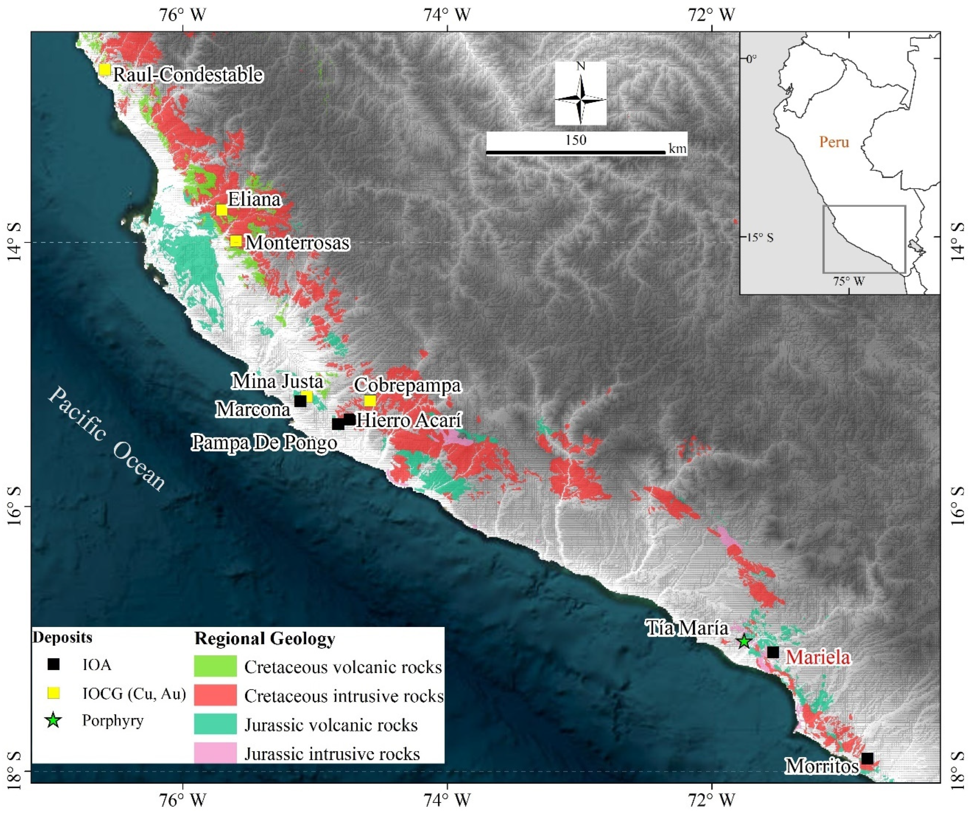
2. Geological Setting

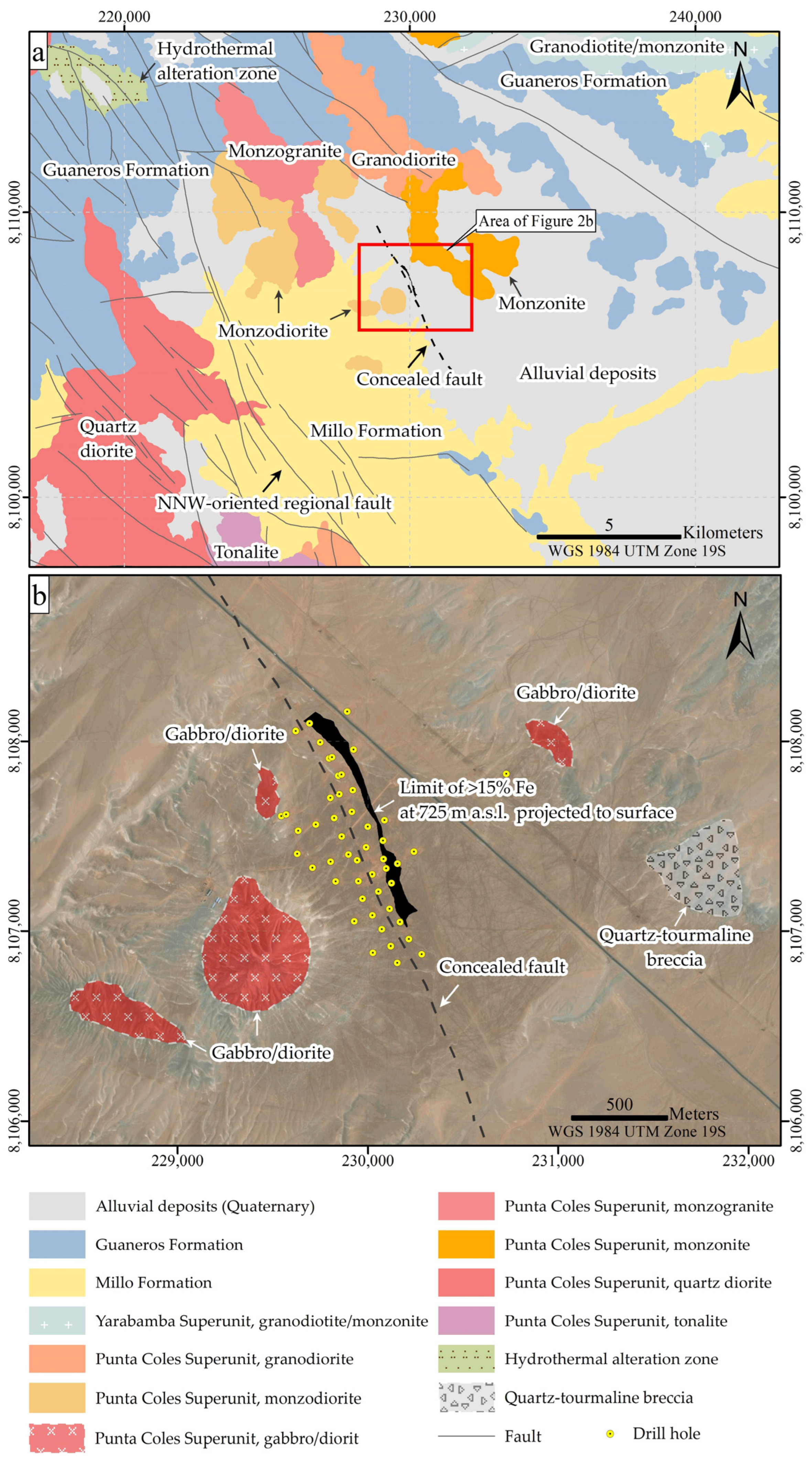
The region of southwestern Peru mainly consists of granulite to amphibolite grade gneisses of the Arequipa Massif [33], which are intruded by the Peruvian Coastal Batholith, composed of over 1000 plutonic bodies [34,35]. These intrusions are distributed along a 1600 km-long and 60 km-wide array, located 150–200 km from the present-day trench [36]. The Early Jurassic to Cretaceous plutonism generated under extensional conditions, with a predominant mantle source and a lack of appreciable crustal contamination, was closely associated with widespread and repeated normal faulting in the back-arc region [34].

The most significant portion of the PIB is located in the southwest of Peru (Figure 1) and contains diverse types of mineral deposits, including stratabound Fe(-Cu), porphyry Cu(-Au), iron oxide-copper-gold (IOCG), and iron oxide-apatite (IOA) deposits [2,33,35,37,38,39,40,41]. Most of the IOA and IOCG deposits are spatially associated with coeval Mesozoic intrusions [2,37]. Different terms have been used to classify the iron deposits (e.g., Marcona, Pamba de Pongo, Morritos) in this region, such as massive magnetite deposit, skarn, or manto type [2,38]. However, a broader classification categorizes them as Kiruna-type iron-oxide-apatite (IOA) deposits [38]. In comparison with the Chilean Iron Belt (CIB) [2], relatively few IOA deposits have been discovered in the PIB. Nevertheless, IOA-like iron occurrences are intermittently distributed throughout the entire PIB.

3. Deposit Geology

The Mariela iron deposit is located at 17°06′ S and 71°32′ W in the desert of Pampa de Clemecí, approximately 29 km west of Yarabamba village (Figure 2a). The deposit is currently owned by Total Genius Iron Mining S.A.C. with estimated resources of 109 Mt at an average grade of 32.6% Fe.

The Mariela deposit is hosted in the intrusions of the Punta Coles Superunit, which is composed of several intrusive bodies with gabbro/diorite, granodiorite, monzodiorite, monzogranite, monzonite, and quartz diorite lithologies (Figure 2a). The mineralization body is covered and concealed by Quaternary deposits (Figure 2a,b). Gabbro-diorite intrusions are the major host rocks of the ore body and have undergone alteration to actinolite, chlorite, and epidote, along with minor amounts of sericite and unspecified clays.

A NNW-oriented magnetite mineralization zone characterizes the Mariela deposit, with a concealed fault aligned with the regional fault being interpreted based on the mineralization orientation (Figure 2a,b). The iron ore can be classified as massive, brecciated, parallel-veined, stockworked, or disseminated. These bodies may exhibit abrupt or gradual contacts in relation to the host rock. The ore mainly consists of magnetite, actinolite, and apatite. Minor sulfides, such as pyrite and chalcopyrite, and copper have been locally observed. Subvertical massive ore bodies with up to 100 m of thickness show sharp contacts with the host rock, although indistinct contacts between the ore body and the host rock are also common. Disseminated magnetite mineralization is common in the host rock surrounding the main mineralization zone, which could also be a significant contributor to the ore deposit.

Mapping and drill core logging for the project revealed three main mineralization/alteration stages at Mariela: massive magnetite, disseminated/veinlet magnetite, and supergene stage (Figure 3). Apatite-rich massive ore blocks (5–30 cm) are commonly observed enclosed within apatite-poor massive magnetite mineralization, indicating early-stage apatite formation. Hence, the massive magnetite stage, characterized by the formation of high-grade massive ore, can be divided into two sub-stages: Sub-stage I and Sub-stage II. Sub-stage I formed ore with a mineral assemblage of magnetite, apatite, and actinolite, while Sub-stage II formed ore characterized by abundant actinolite and lesser amounts of apatite. The disseminated/veinlet magnetite stage led to the formation of disseminated/veinlet magnetite and the presence of minor hydrothermal quartz and sulfides, accompanied by intense hydrothermal alteration and the occurrence of minerals such as albite, chlorite, epidote, calcite, clay minerals, etc. In the supergene stage, a partial volume of hematite (1%–90%) formed in the near-surface portion of the deposit ore, along with the formation of secondary minerals such as Cu carbonates and jarosite.

Hydrothermal alteration is defined by a pervasive actinolitization around the magnetite ore, grading outward to an albitization zone. To the southeast, a tourmaline-quartz zone is outcropped (Figure 2b). Post-mineral dikes striking NNW have been observed in the drill cores and eastern part of the deposit.

4. Samples and Analytical Methods

Different samples were collected from various drill holes in the massive magnetite and disseminated mineralization zones. Thin and thick sections were prepared for petrographic observation using an optical microscope and scanning electron microscope (SEM). The selected samples are representative of the main styles of mineralization. Massive magnetite ore samples Mt-01 and Mt-02 were selected for EPMA and LA-ICP-MS analysis to represent the mineralization during Sub-stage I and Sub-stage II, respectively. Mt-01 is characterized by a mineral assemblage of magnetite + actinolite + apatite, while Mt-02 has a mineral assemblage of magnetite + actinolite. Additionally, a host rock sample (Mt-03), which was strongly altered with abundant disseminated magnetite, was also analyzed by LA-ICP-MS to represent the chemical composition of magnetite from relatively low-grade ore.

Major element compositions of magnetite were determined at the MNR Key Laboratory of Metallogeny and Mineral Assessment, Institute of Mineral Resources, Chinese Academy of Geological Sciences, with a JXA-iHP200F Electron Probe Micro Analyzer (EPMA; JEOL, Tokyo, Japan) equipped with five wavelength-dispersive spectrometers. The samples were coated with a ca. 20 nm thin conductive carbon film prior to analysis. Details of EPMA methods are described by Yang et al. [45]. During the analysis, an accelerating voltage of 20 kV, a beam current of 20 nA, and a 1 µm spot size were used to analyze minerals. Natural minerals and alloys were used as standards (Supplementary Table S1). Data were corrected online using a modified ZAF (atomic number, absorption, fluorescence) correction procedure. In addition to quantitative spot analyses, qualitative wavelength dispersive X-ray maps (WDS) of Mg, Al, Ce, Sr, Fe, Ti, V, and Cr were obtained for selected magnetite grains. The mapping was performed with a 10 kV acceleration voltage and 100 nA beam current. The peak position measurement time was 50 s, and the background time was 25 s. The detailed instrument settings and operation procedures used were similar to those described by Yang et al. [45].

Detailed trace and major element concentrations in magnetite were measured by Laser Ablation Inductively Coupled Plasma Mass Spectrometry (LA-ICP-MS) on polished thick thin sections at the MNR Key Laboratory of Metallogeny and Mineral Assessment, Institute of Mineral Resources, Chinese Academy of Geological Sciences. The analyses were carried out on an Agilent 7900 Quadrupole ICP-MS (Santa Clara, CA, USA) coupled to a Photon Machines Analyte HE 193-nm ArF Excimer Laser Ablation system (ESL, Florida, United States). Argon was used as the make-up gas and mixed with the carrier gas via a T-connector before entering the ICP [46,47]. The concentrations of Li, Be, B, Na, Mg, Al, Si, P, S, K, Ca, Sc, Ti, V, Cr, Mn, Fe, Co, Ni, Cu, Zn, Ga, Ge, As, Rb, Sr, Y, Zr, Nb, Mo, Cd, In, Sn, Sb, Cs, Ba, La, Ce, Pr, Nd, Sm, Eu, Gd, Tb, Dy, Ho, Er, Tm, Yb, Lu, Hf, Ta, W, Tl, Pb, Bi, Th, and U were measured in magnetite. Each analysis was performed with a spot diameter of 32 μm at 8 Hz with an energy of ~4 J/cm² for 40 s after measuring the gas blank for 20 s. Standard reference materials GSE-1g, GSD-1g, BCR-2G, and NIST 610 were used as external standards to plot the calibration curve. The preferred values of element concentrations for the USGS reference glasses are from the GeoReM database [48]. Standard reference materials were run after each of the 10–15 unknowns; detection limits were calculated for each element in each spot analysis. The off-line data processing was performed in ICPMSDataCal [49].

5. Results

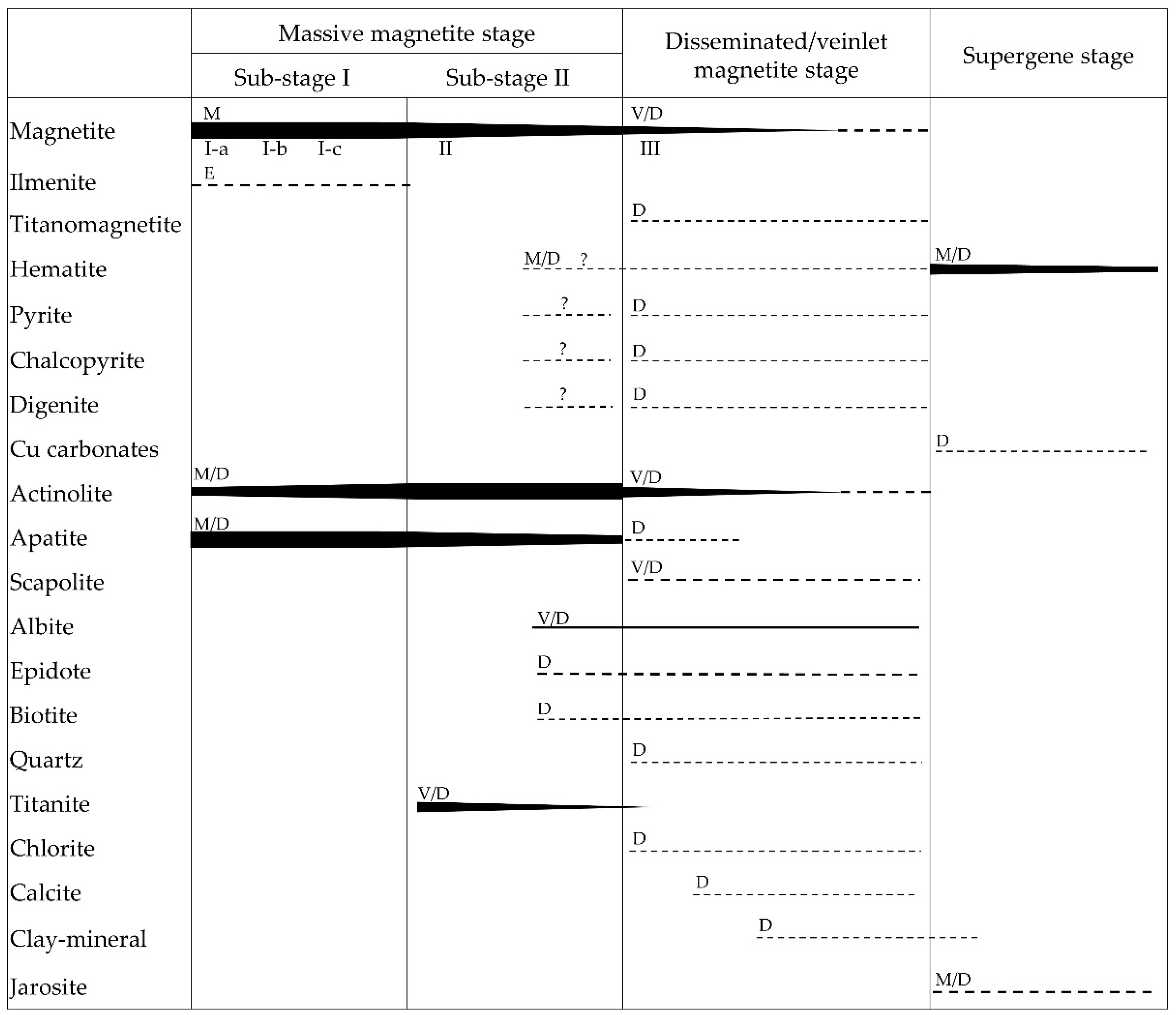
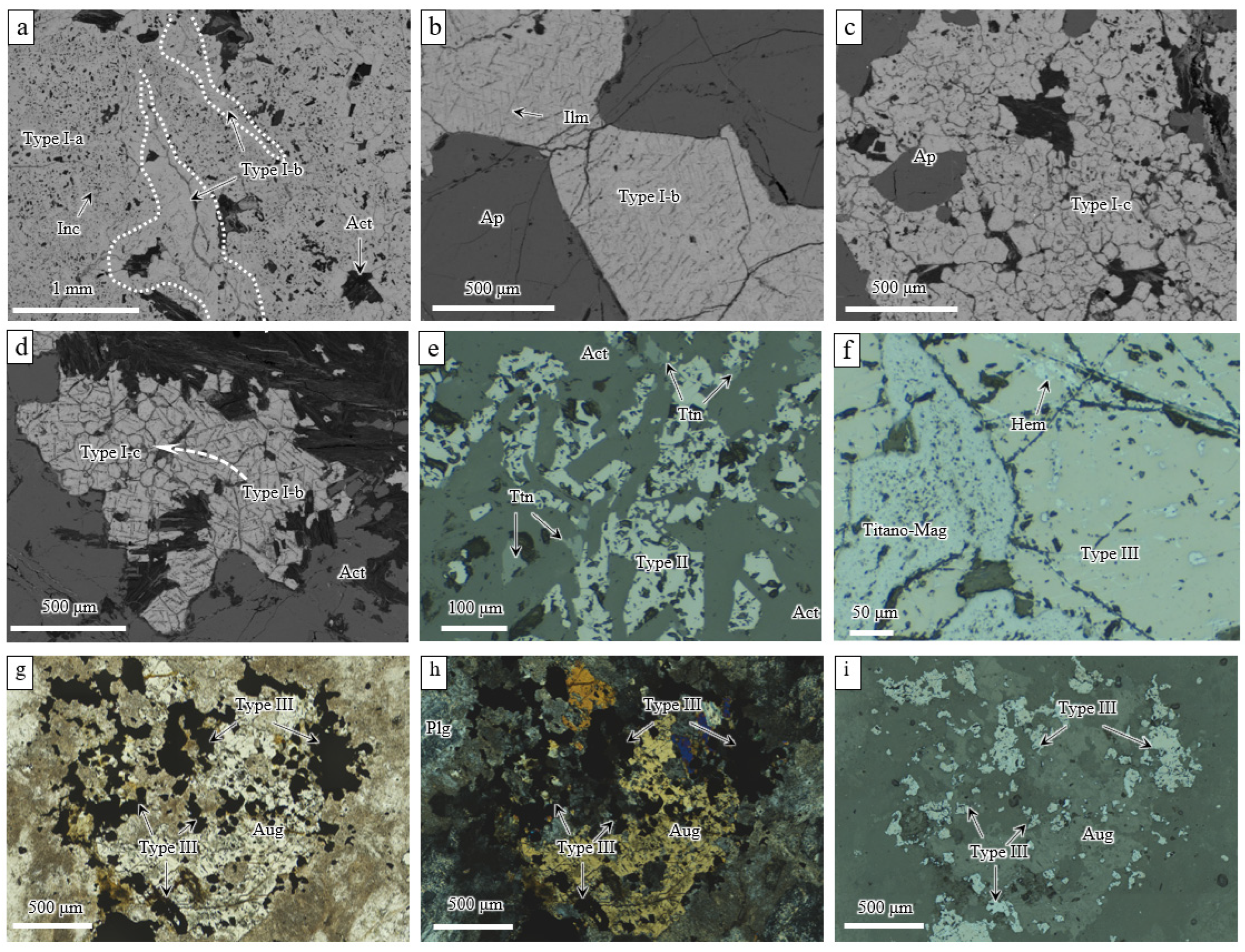
5.1. Magnetite Textures

Three main types of magnetite were identified based on spatial location, paragenesis (Figure 3), and typical micro-textures. Type I and Type II magnetite, occurring in high-grade massive magnetite ores, correspond to Sub-stage I and Sub-stage II of the massive magnetite stage, with Type I characterized by a mineral assemblage of magnetite + actinolite + apatite and Type II characterized by a magnetite + actinolite assemblage (Figure 3;

Table 1. Summary of the main magnetite types and typical microtextures at Mariela.

Mineralization Type	Mineral Assemblage	Magnetite Type		Main Feature/Typical Microtexture
High-grade massive magnetite bodies	Mag + Act + Ap	Type-I	Type I-a	Inclusion-rich magnetite
			Type I-b	Inclusion-poor magnetite with well-developed ilmenite exsolution lamellae
			Type I-c	Inclusion-poor magnetite with minor ilmenite exsolution lamellae, characterized by mosaic texture
	Mag + Act + Ttn	Type II		Inclusion-rich to inclusion-poor magnetite
Low-grade disseminated magnetite ore in host rock	Mag + Titano − Mag ± Hem	Type III		Inclusion-poor, minor ilmenite exsolution lamellae, partly oxidized by hematite

Abbreviations: Mag (magnetite), Act (actinolite), Ap (apatite), Hem (hematite), Titano-Mag (titanomagnetite).

). The Type II magnetite sample has significantly less apatite compared to Type I. According to the microstructure, Type I is further subdivided into three subclasses: Type I-a, I-b, and I-c, as summarized in Table 1. Type I-a magnetite contains abundant mineral inclusions ranging in size from <1 μm to ~35 μm and aligned along magnetite crystallographic planes or randomly distributed (Figure 4a). Some lager inclusions can be recognized as silicate minerals, e.g., actinolite (Figure 4a). Type I-b magnetite is generally inclusion-free with well-developed ilmenite exsolution lamellae (Figure 4b). Type I-c magnetite is inclusion-poor with minor ilmenite exsolution lamellae and displays a mosaic texture, which is characterized by well-defined 120° triple junctions (Figure 4c,d). Type II magnetite, which is associated with abundant actinolite (up to 40 vol.%) and titanite (up to 2 vol.%), is also inclusion-bearing but appears to contain fewer inclusions than Type I-a (Figure 4e). Type III magnetite occurs in relative low-grade ore, is inclusion-poor, and shows minor ilmenite exsolution lamellae (Figure 3 and Figure 4f–i).

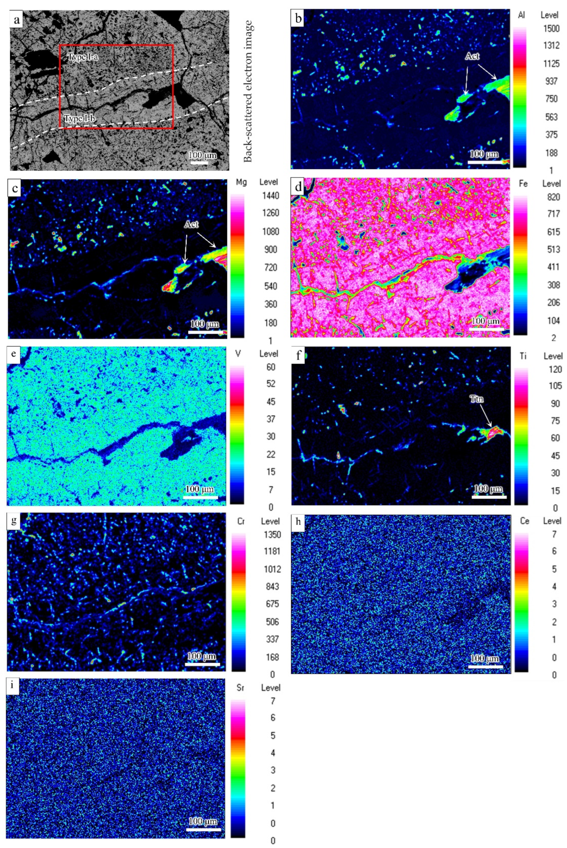
5.2. WDS X-ray Elemental Maps

The distribution of Mg, Al, Ce, Sr, Fe, Ti, V, and Cr within selected magnetite grains was determined by making WDS X-ray maps (Figure 5). Type I-a magnetite is slightly more enriched in Fe, Mg, Al, and Cr (Figure 5b–d,g) and has more Mg- and Al-rich mineral inclusions (<10 μm; Figure 5b,c). Type I-b magnetite is distributed on both sides of microfractures and associated with larger Mg- and Al-rich minerals (e.g., actinolite) and Ti-rich minerals (e.g., ilmenite) in the fractures (Figure 5b,c,f). Minerals with high Ti and Cr content and low V content are distributed in a linear and staggered pattern (Figure 5a,f), which may have resulted from the precipitation of ilmenite along the lattice of Type I-b magnetite. Magnesium, Ti, and Cr are relatively enriched in the fractures, where Fe and V are depleted (Figure 5c–g). The distribution patterns of Sr and Ce are not clear due to their low content in the samples analyzed by spectral mapping (Figure 5h,i).

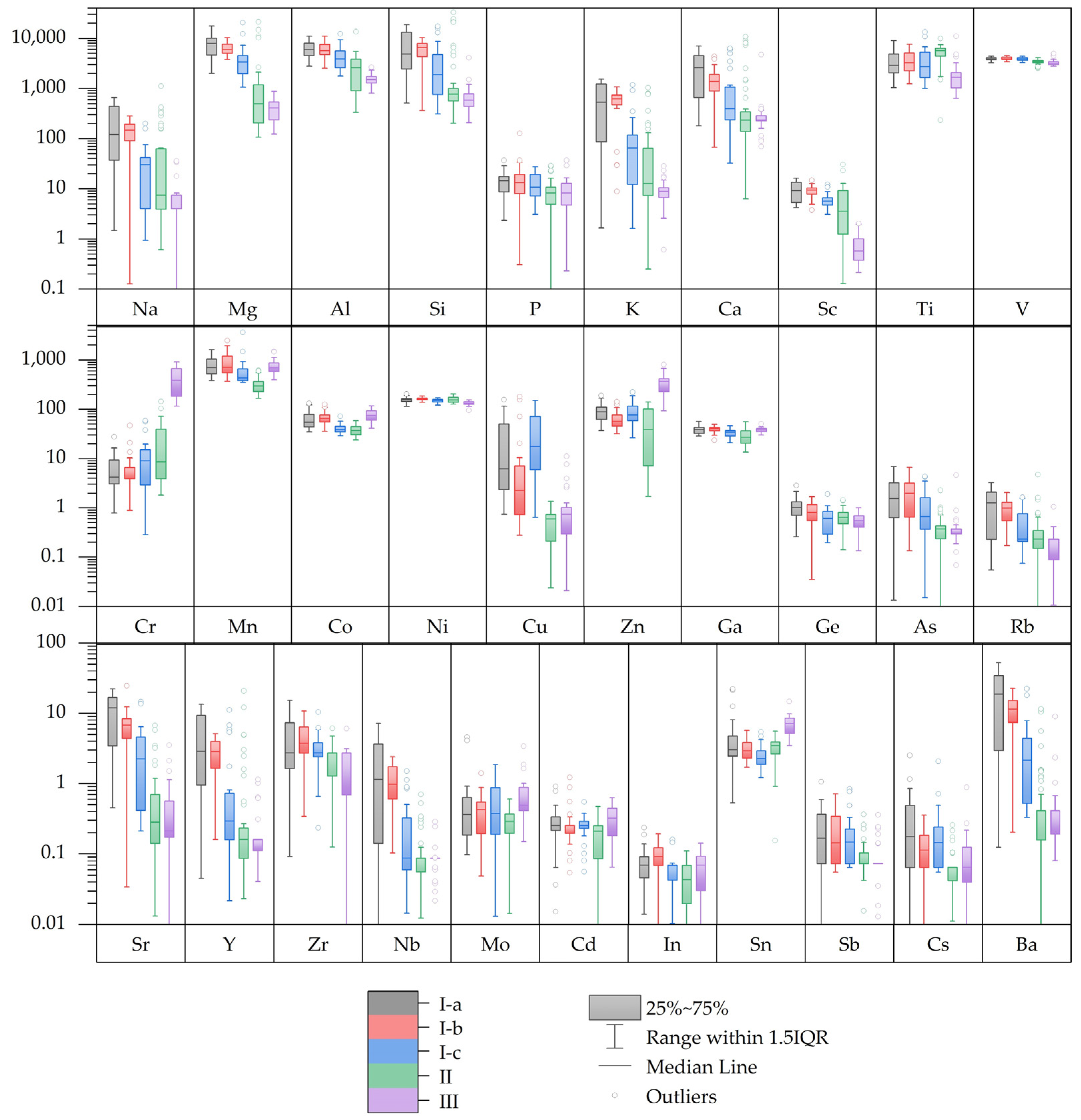
5.3. Magnetite Chemistry

The EPMA data are reported in Supplementary Table S2, and a statistical summary for each magnetite type, including minimum, maximum, and average (avg.) compositions, is presented in

Table 2. Data summary of EPMA analyses for Type I and II magnetite from Mariela.

	n	Types I and II N = 51	n	Type I-a N = 16	n	Type I-b N = 15	n	Type I-c N = 10	n	Type II N = 10
MgO	51	0.01–1.56	16	0.07–1.56	15	0.02–0.66	10	0.09–0.9	10	0.01–1.33
		0.40		0.48		0.30		0.28		0.52
Al2O3	51	0.16–3.26	16	0.28–1.26	15	0.16–1.36	10	0.24–1.32	10	0.34–3.26
		0.80		0.60		0.72		0.64		1.41
SiO2	37	BDL-2.98	12	BDL-2.98	13	BDL-1.27	5	BDL-2.14	7	BDL-1.01
		0.41		0.65		0.42		0.28		0.13
TiO2	49	BDL-1.96	15	BDL-1.96	15	0.02–0.6	9	BDL-0.45	10	0.03–1.3
		0.35		0.28		0.3		0.18		0.72
V2O3	51	0.57–0.79	16	0.61–0.79	15	0.66–0.79	10	0.57–0.69	10	0.66–0.75
		0.70		0.70		0.72		0.64		0.72
MnO	43	BDL-0.43	13	BDL-0.43	11	BDL-0.12	9	BDL-0.16	10	0.01–0.18
		0.07		0.08		0.05		0.06		0.11
Cr2O3	47	BDL-4.84	15	BDL-0.27	14	BDL-0.21	9	0–4.84	9	BDL-0.11
		0.19		0.09		0.05		0.71		0.05
FeO	51	82.60–91.51	16	84.54–91.51	15	87.98–90.9	10	82.6–91.33	10	85.17–90.43
		88.45		88.01		89.25		88.32		88.07
Total	51	88.36–94.26	16	88.36–93.49	15	89.67–94.26	10	89.2–93.24	10	89.78–93.03
		91.74		91.33		92.18		91.53		91.95

Note: All concentrations are reported in wt.%. The range indicates the minimum and maximum concentrations. The average is shown in italics. The low totals are due to expressing all Fe as FeO in the analyses. BDL = below detection limit; N = total number of analyses; n = number of analyses above the detection limit.

. The important compositional variations occur for Mg, Al, Si, Ti, V, Mn, Cr, and Fe (avg. wt.% in oxide components: 0.40% MgO; 0.80% Al₂O₃; 0.41% SiO₂; 0.35% TiO₂; 0.70% V₂O₃; 0.07% MnO; 0.19% Cr₂O₃; and 88.45% FeO (Table 2; Supplementary Table S2)). Other element concentrations are below or close to the detection limits (Supplementary Tables S1 and S2). The distribution of Ca in magnetite is uneven, with more than half of the tested points below the detection limit. The contents of other elements, e.g., Cr, Zn, and Nb, are very low or below the detection limits (Table 2; Supplementary Table S2). The Si concentration in Type I-a magnetite averages 0.65 wt.% in SiO₂, which is higher than that of Type I-b, Type I-c, and Type II magnetite, with average wt.% in SiO₂ of 0.42, 0.28, and 0.13, respectively. This may be related to the presence of more fine mineral inclusions in Type I-a magnetite (Figure 5a–g). In Type I-b magnetite, the concentration of Cr (up to 4.84 wt.% Cr₂O₃) is locally high, which may be caused by the presence of local Cr-bearing mineral inclusions.

The LA-ICP-MS data are reported in Supplementary Table S3, and a corresponding statistical summary is presented in

Table 3. Data summary of LA-ICP-MAS analyses for Types I and II magnetite from Mariela.

	n	Type I-a N = 27	n	Type I-b N = 28	n	Type I-c N = 24	n	Type II N = 50	n	Type III N = 27
Li	12	BDL-7.72	17	BDL-13.66	9	BDL-9.77	23	BDL-4.04	13	BDL-6.14
		4.68		4.58		5.29		1.39		2.36
Be	16	BDL-73.37	12	BDL-46.48	10	BDL-71.94	32	BDL-54.1	18	BDL-24.22
		35.42		25.21		33		12.66		9.16
B	24	BDL-44.27	26	BDL-28.26	16	BDL-28.53	32	BDL-29.16	16	BDL-151.07
		19.88		13.69		8.4		5.13		10.92
Na	27	1.48–665.86	26	BDL-283.58	19	BDL-199.35	43	BDL-1113.3	16	BDL-35.63
		231.65		151.75		46.9		90.72		8.55
Mg	27	2001.47–17,387.43	28	3782.17–10,372.6	24	1056.69–20,441.77	50	106.83–21,150.2	27	124.38–872.03
		7849.28		6537.62		4346.13		1791.13		412.29
Al	27	2807.18–11,097.43	28	2552.75–11,056.85	24	1768.36–12,304.28	50	336.31–13,599.17	27	806.32–2670.33
		6224.15		6119.84		4498.06		2584.48		1571.15
Si	27	515.22–18,537.94	28	364.89–10,353.44	24	310–17,246.91	49	BDL-33,105.92	27	206.2–4100.49
		8063.86		5966.28		4045.7		3166.41		747.45
P	26	BDL-36.77	25	BDL-129.06	19	BDL-27.65	43	BDL-29.13	22	BDL-36.98
		15.49		18.83		14.42		9.26		10.64
S	26	BDL-1344.34	28	43.54–641.36	23	BDL-796.43	24	BDL-416.31	27	71.98–415.59
		366.82		377.23		319.44		259.57		238.34
K	27	1.66–1530.72	26	BDL-1069.36	21	BDL-1180.26	46	BDL-1039.13	18	BDL-28.69
		653.67		623.08		179.19		97.22		10.09
Ca	25	BDL-7050.88	28	66.87–4351.46	21	BDL-6306.07	35	BDL-10,822.33	18	BDL-4720.42
		2702.28		1483.14		1443.73		1382.08		489.05
Sc	27	4.23–16.23	28	3.77–14.84	24	3.09–12.2	49	BDL-30.91	27	0.22–2.02
		9.45		8.99		6.07		5.62		0.79
Ti	27	1027.83–9021.98	28	1237.91–7691.56	24	992.26–13,383.99	50	234.81–9996.54	27	640.72–11,064.64
		3594.07		3662.45		3946.42		5290.79		2121.84
V	27	3263.33–4394.73	28	3439.14–4515.97	24	3290.85–4414.2	50	2549.88–4116.67	27	2784.15–4946.98
		3899.12		3954.37		3864.29		3436.53		3320.95
Cr	23	BDL-27.82	20	BDL-46.65	23	BDL-58.26	32	BDL-143.47	27	115.85–914.89
		7.04		8.07		13.71		35.42		426.88
Mn	27	380.89–1608.65	28	368.03–2464.4	24	350.57–3631.22	50	167.22–619.33	27	397.99–1476.4
		772.29		924.85		669.14		315.51		767.13
Fe	27	64.61–73.59	28	67.97–73.12	24	63.49–73.88	50	62.6–74.21	27	70.66–74.54
		69.51		70.28		71.42		72.31		73.93
Co	27	34.92–132.39	28	35.81–126.16	24	29.2–71.88	50	23.81–58.26	27	41.68–116.32
		63.84		69.94		41.7		38.55		77.38
Ni	27	113.88–204.09	28	137.81–186.59	24	121.53–171.26	50	126.64–205.12	27	94.97–154.43
		156.98		162.84		149.56		158.43		133.44
Cu	25	BDL-155.68	24	BDL-180.32	21	BDL-150.71	33	BDL-1.36	20	BDL-11.06
		32.26		20.94		47.34		0.43		1.76
Zn	27	37.23–189.31	28	31.94–142.89	24	26.26–222.87	50	1.72–140.77	27	93.1–813.98
		91.64		64.48		92.18		56.47		353.23
Ga	27	28.59–56.22	28	23.68–49.09	24	20.84–46.04	50	13.51–55.34	27	30.1–50.24
		38.44		39.67		33.81		29.11		38.23
Ge	26	BDL-2.84	28	0.03–1.69	21	BDL-1.91	50	0.14–1.45	27	0.13–1
		1.09		0.89		0.71		0.67		0.55
As	25	BDL-6.93	28	0.13–6.63	20	BDL-4.36	33	BDL-2.28	14	BDL-4.63
		2.13		2.25		1.34		0.43		0.64
Rb	23	BDL-3.24	26	BDL-2.06	18	BDL-1.65	30	BDL-4.72	16	BDL-1.06
		1.48		1.04		0.56		0.55		0.19
Sr	27	0.45–211.61	27	BDL-24.64	22	BDL-14.68	48	BDL-358.5	17	BDL-3.52
		17.58		7.12		3.98		8.26		0.68
Y	27	0.04–13.47	24	BDL-5.11	20	BDL-11.16	34	BDL-20.93	15	BDL-1.15
		5.49		3.14		1.78		1.66		0.31
Zr	21	BDL-15.33	22	BDL-10.76	16	BDL-10.4	28	BDL-6.14	17	BDL-6.11
		4.8		4.85		3.52		1.87		1.68
Nb	26	BDL-7.24	28	0.1–2.42	19	BDL-1.51	30	BDL-0.7	11	BDL-0.29
		2.17		1.13		0.34		0.14		0.1
Mo	27	0.1–4.58	28	0.05–1.41	24	0.01–1.87	49	BDL-0.6	27	0.15–3.4
		0.67		0.43		0.56		0.29		0.74
Cd	20	BDL-0.91	17	BDL-1.23	13	BDL-0.55	38	BDL-0.47	23	BDL-0.63
		0.32		0.32		0.26		0.17		0.34
In	17	BDL-0.24	21	BDL-0.19	12	BDL-0.16	38	BDL-0.11	21	BDL-0.14
		0.08		0.11		0.06		0.04		0.06
Sn	27	0.53–22.19	28	1.72–5.73	24	1.22–5.45	50	0.16–5.58	27	3.46–14.83
		5.14		3.1		2.54		3.23		7.09
Sb	23	BDL-1.07	20	BDL-0.72	17	BDL-0.84	29	BDL-0.36	11	BDL-0.36
		0.28		0.3		0.27		0.11		0.13
Cs	23	BDL-2.52	22	BDL-0.36	18	BDL-2.08	25	BDL-0.26	21	BDL-0.88
		0.43		0.14		0.34		0.06		0.12
Ba	26	BDL-52.68	28	0.2–22.47	19	BDL-22.31	28	BDL-11.55	14	BDL-8.99
		20.85		11.21		4.72		1.52		1.08
La	26	BDL-9.18	27	BDL-8.69	23	BDL-7.61	38	BDL-2.74	23	BDL-1.79
		3.75		2.74		2.13		0.39		0.35
Ce	27	0.13–28.96	28	0.08–21.14	24	0.01–23.8	44	BDL-14.11	19	BDL-47.66
		11.65		7		4.18		1.2		3.26
Pr	26	BDL-3.95	28	0.01–2.76	21	BDL-3.79	35	BDL-2.8	15	BDL-0.41
		1.64		0.97		0.8		0.27		0.12
Nd	26	BDL-16.07	28	0.05–11.09	20	BDL-20.07	33	BDL-14.28	16	BDL-1
		6.88		4.34		3.69		1.38		0.33
Sm	22	BDL-3.31	27	BDL-1.83	14	BDL-3.07	18	BDL-5.42	12	BDL-0.25
		1.69		0.93		0.94		0.75		0.14
Eu	23	BDL-0.52	22	BDL-0.29	17	BDL-0.34	28	BDL-0.41	16	BDL-0.12
		0.22		0.11		0.14		0.07		0.04
Gd	23	BDL-3.17	25	BDL-1.6	16	BDL-2.62	23	BDL-5.28	13	BDL-0.24
		1.4		0.73		0.62		0.58		0.1
Tb	25	BDL-0.4	25	BDL-0.26	12	BDL-0.21	24	BDL-0.6	11	BDL-0.06
		0.16		0.1		0.08		0.08		0.02
Dy	23	BDL-2.71	24	BDL-1.16	16	BDL-2.07	20	BDL-4.12	15	BDL-0.59
		1.27		0.57		0.43		0.59		0.1
Ho	23	BDL-0.72	23	BDL-0.3	14	BDL-0.45	26	BDL-0.74	17	BDL-0.04
		0.26		0.12		0.1		0.09		0.02
Er	24	BDL-1.85	22	BDL-0.97	19	BDL-1.03	23	BDL-2.25	17	BDL-0.15
		0.63		0.36		0.23		0.24		0.05
Tm	20	BDL-0.23	25	BDL-0.16	15	BDL-0.19	23	BDL-0.22	14	BDL-0.19
		0.1		0.07		0.06		0.04		0.03
Yb	24	BDL-1.24	24	BDL-0.62	18	BDL-1.36	23	BDL-2.34	13	BDL-0.21
		0.56		0.32		0.35		0.34		0.09
Lu	23	BDL-0.26	27	BDL-0.13	16	BDL-0.22	30	BDL-0.14	19	BDL-0.05
		0.08		0.04		0.06		0.03		0.02
Hf	24	BDL-0.47	21	BDL-0.52	14	BDL-0.34	30	BDL-0.34	7	BDL-0.22
		0.17		0.19		0.13		0.1		0.08
Ta	23	BDL-0.96	26	BDL-0.43	18	BDL-0.35	36	BDL-0.06	21	BDL-0.04
		0.35		0.23		0.09		0.02		0.01
W	24	BDL-2.06	21	BDL-0.71	21	BDL-2.43	30	BDL-2.46	16	BDL-0.52
		0.39		0.18		0.45		0.13		0.13
Tl	10	BDL-0.06	8	BDL-0.04	7	BDL-0.03	19	BDL-0.04	15	BDL-0.04
		0.03		0.02		0.02		0.01		0.01
Bi	14	BDL-0.1	15	BDL-0.13	17	BDL-0.13	21	BDL-0.06	19	BDL-0.09
		0.04		0.04		0.04		0.03		0.03
Pb	26	BDL-3.21	27	BDL-3.78	22	BDL-1.41	37	BDL-0.34	19	BDL-17.44
		0.85		0.75		0.51		0.08		3.09
Th	27	0.01–8.41	28	0.01–1.74	24	0.02–12.23	27	BDL-1.56	10	BDL-1.08
		2.41		0.85		1.07		0.21		0.16
U	25	BDL-4.02	26	BDL-2	24	0.01–7.87	36	BDL-4.59	12	BDL-0.69
		1.33		0.69		1.04		0.28		0.22

Note: All concentrations are reported in ppm except Fe in wt.%. The range indicates the minimum and maximum concentrations. The average is shown in italics. BDL = below detection limit; N = total number of analyses; n = number of analyses above the detection limit.

. Among the five types/sub-types of magnetite, the high-content trace elements include Mg, Al, Mn, Ti, V, and Co, with average contents of 3846.02 ppm, 3967.99 ppm, 636.51 ppm, 3949.56 ppm, 3655.34 ppm, and 55.77 ppm, respectively (Supplementary Table S3). Other elements with relatively high contents include Ni, Zn, Cr, Ga, Cu, Sr, Ba, Ce, and Sn, with average contents of 153.28 ppm, 120.85 ppm, 106.38 ppm, 34.92 ppm, 19.13 ppm, 8.24 ppm, 8.72 ppm, 5.11 ppm, and 4.10 ppm, respectively (Table 3; Supplementary Table S3). The average contents of the remaining trace elements were all below 4 ppm (Supplementary Table S3). The ΣREE average was 11.77 ppm, with an average LREE value of 10.22 ppm and a low HREE average of only 1.55 ppm (Supplementary Table S3).

Nickel, V, Co, and Ga contents in different types of magnetite are relatively consistent and stable (Table 3; Figure 6). The Na, Mg, Al, Si, Ca, Ba, Ge, Sr, and Y elements exhibited a trend of enrichment to gradual depletion from Type I-a to Type III magnetite (Table 3; Figure 6). Types I-a and I-b magnetite show similar trace element contents, but Type I-b magnetite is slightly more enriched in Ga and Mn and depleted in Al, Mg, Zn, Ba, Cu, and Ge (Table 3; Figure 6). The element contents in Type I-c magnetite are generally within the transitional ranges of Types I-a, I-b, II, and III magnetite (Table 3; Figure 6). Type III magnetite shows a deficiency in Mn (avg. 313.04 ppm) compared to the other four types of magnetite. Type III magnetite is significantly enriched in Cr (avg. 418.01 ppm) and Zn (avg. 353.23 ppm) compared with other magnetite but relatively deficient in Al, Mg, Ti, Ba, Ge, and Sr (average values: 1743.41 ppm Al; 400.28 ppm Mg; 2075.11 ppm Ti; 2.09 ppm Ba; 0.55 ppm Ge; 1.98 ppm Sr; Table 3; Figure 6).

6. Discussion

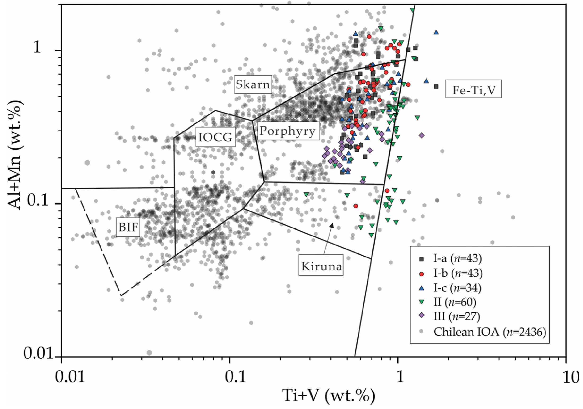
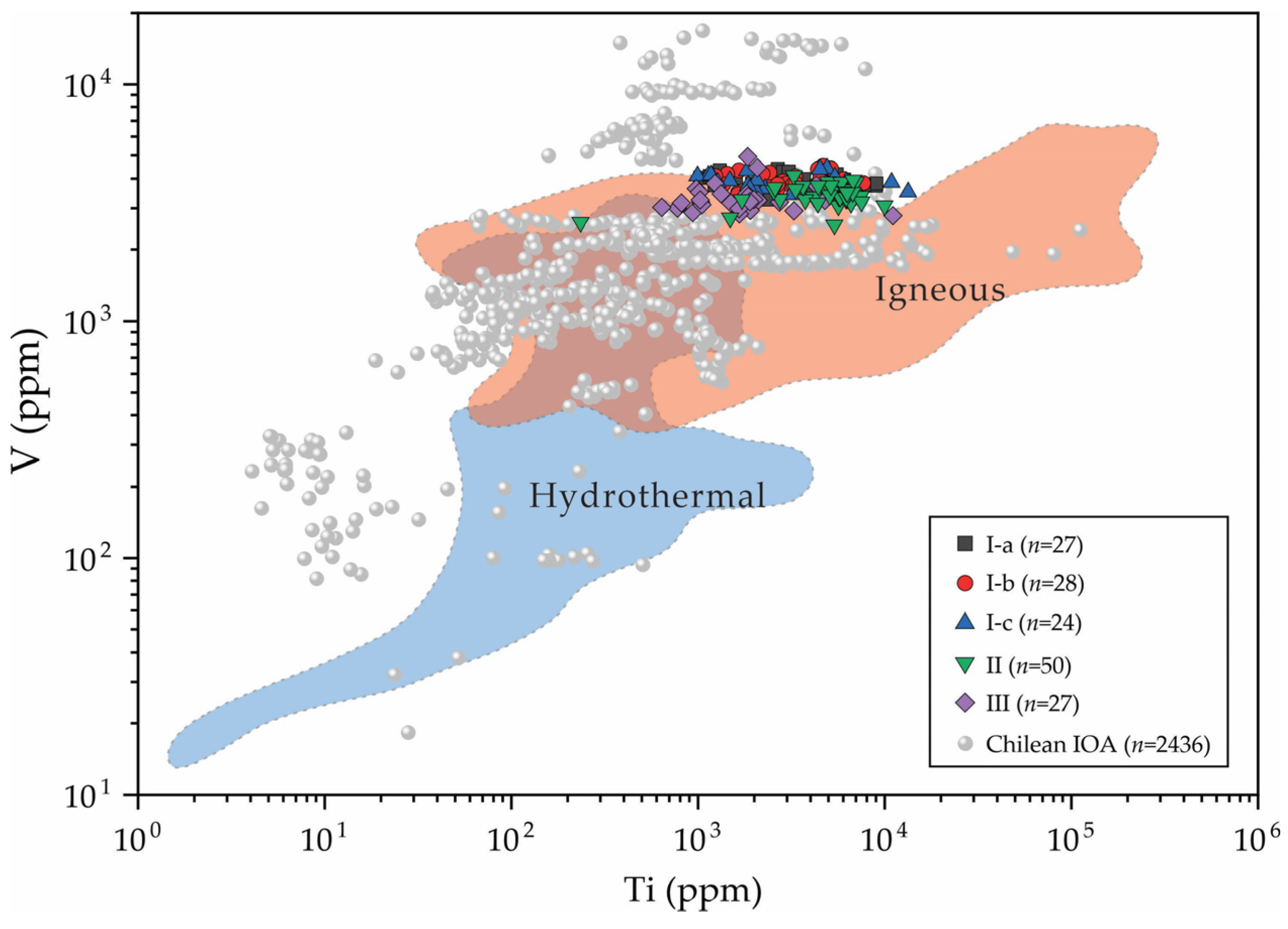
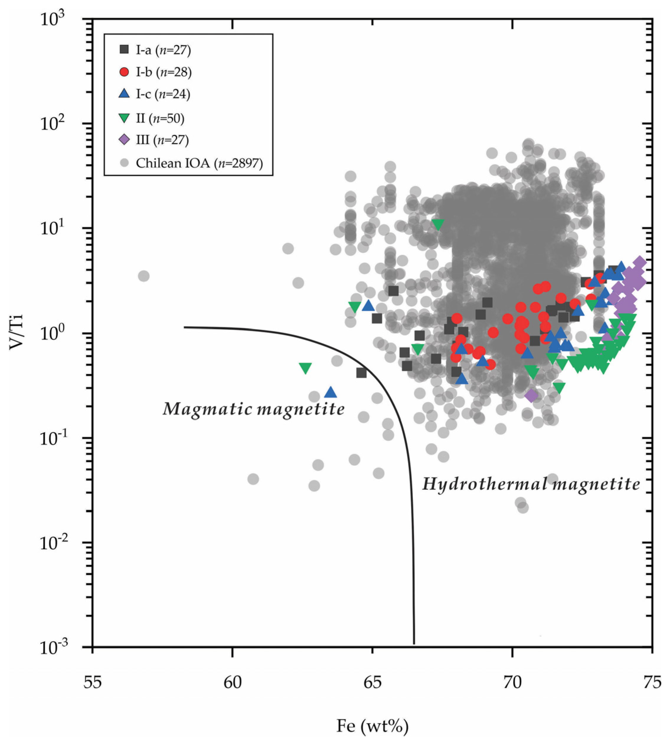
6.1. Magmatic to Hydrothermal Transition

Magnetite is one of the most important ore minerals in IOA deposits. Due to the numerous minor and trace element (e.g., Al, Ti, Mg, Mn, Zn, Cr, V, Ni, Co, and Ga) substitutions that can occur in spinel group minerals such as magnetite, distinct trace element signatures can arise under different conditions [19,20,21,50,51]. Several discrimination diagrams based on trace element data have been proposed to differentiate between igneous and hydrothermal magnetite [14,15,52,53,54]. In this study, we selected the [Ti + V] vs. [Al + Mn], Ti vs. V, and V/Ti vs. Fe (wt.%) discrimination diagram to constrain the ore-forming environment of the Mariela deposit.

Data obtained from Mariela and previous studies on Chilean IOA deposits were used to plot the [Ti + V] vs. [Al + Mn] discrimination diagram (Figure 7). Types I-a, I-b, and I-c have similar [Ti + V] concentrations (e.g., avg. 0.73 wt.%, 0.71 wt.%, and 0.71 wt.%, respectively). Type II has a higher [Ti + V] concentration of avg. 0.88 wt.%, and disseminated Type III magnetite shows a lower concentration of avg. 0.54 wt.%. The [Al + Mn] concentration decreases gradually from Type I-a to Type III (0.60–0.23 wt.%). Type II shows a wide range of [Al + Mn] contents (0.06–1.85 wt.%). In summary, most of the analyses of Mariela magnetite grains were plotted in the porphyry and Fe-Ti, V fields, and a small portion were plotted in the skarn and Kiruna fields. In comparison to the Chilean IOA deposit, the magnetite grains from Mariela plot closer to the Fe-Ti, V field, which suggests a relatively higher formation temperature and a closer association with magmatic origin.

Igneous magnetite commonly has higher V and Ti concentrations than hydrothermal magnetite [16,18,52]. LA-ICP-MS data show the Mariela magnetite contains relatively high and constant V (3263.33–4394.73 ppm) and variable Ti (1027.83–9021.98 ppm; Figure 6; Table 3). All types of magnetite plot mostly in or close to the igneous area on the Ti vs. V diagram (Figure 8). Some Type III magnetite points plot close to the hydrothermal area, suggesting that the disseminated magnetite within the host rock may be more closely associated with hydrothermal processes.

The Fe vs. V/Ti diagram is also used to distinguish between igneous and hydrothermal magnetite [16,18,53]. Magnetite from Mariela mostly plots in the hydrothermal area (Figure 9). The Type III magnetite has a higher V/Ti value than others, and the Type I magnetite (Type I-a, I-b, and I-c) shows a relatively wide range of Fe contents (Figure 9), suggesting a re-equilibration trend, which is supported by the observation of mosaic structure in Type I-c magnetite [16,56,57,58]. The V/Ti ratio for Mariela is relatively stable and close to 1 in comparison to the Chilean IOA deposit (Figure 9).

Trace element concentrations of magnetite are significantly influenced by factors such as temperature, pressure, oxygen and sulfur fugacity, hydrothermal fluid composition, co-precipitation of competing mineral phases, and fluid-rock interactions [16,18]. Importantly, magnetite can undergo metasomatism in hydrothermal fluids, leading to significant modifications in its initial chemical characteristics [59]. Therefore, geochemical diagrams should be used with caution when determining whether magnetite is of magmatic or hydrothermal origin. Field and microscopic observations can provide crucial geological evidence, such as the paragenetic association with hydrothermal minerals, the microstructure of magnetite influenced by re-equilibration processes, the occurrence patterns of magnetite, etc. These observations mutually validate each other in determining the origin of magnetite. Distinguishing between magmatic and high-temperature magmatic-hydrothermal fluid origins can be challenging. The magnetite geochemistry data in the Mariela deposit is plotted into different genetic areas in different geochemical diagrams, indicating a paradox of magmatic and hydrothermal origins. In previous studies, magnetite-rich ores have been attributed to magmatic processes [18,22], whereas hydrothermal fluids may have contributed to the concentration of magnetite and the formation of the deposits through replacement of the host rocks [57].

The inclusion-rich magnetite (Types I-a) from high-grade massive ore could have an initial magmatic or high-temperature magmatic-hydrothermal origin and may have undergone slight modifications due to later hydrothermal processes during transportation and subsequent magnetite precipitation (Types I-b and I-c). The Type II magnetite formed in hydrothermal fluid with the intimate coexistence of abundant actinolite. The disseminated magnetite (Type III) and related veinlet-type magnetite formed last after the fluid replaced the host rock. Abundant disseminated magnetite surrounds altered dark minerals, such as augite (Figure 4g–i), in the host rock, serving as evidence for Fe re-enrichment during the hydrothermal process.

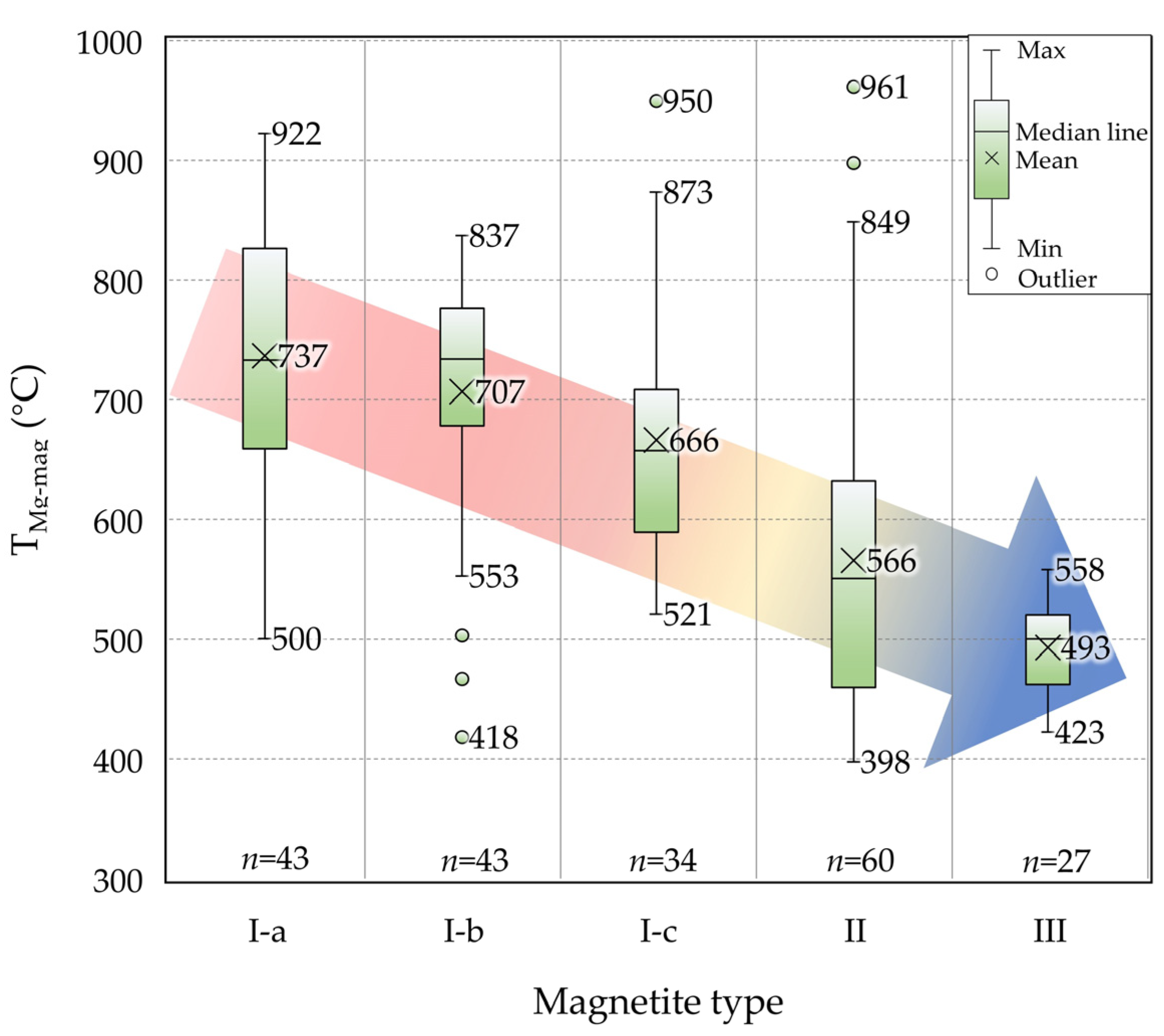
6.2. Temperature of Magnetite Formation

A T_Mg-Mag thermometer was proposed by Canil and Lacourse [60] as a potential method for qualitatively estimating the crystallization temperature of magnetite at the grain scale using the Mg and Fe concentrations in igneous or hydrothermally altered rocks. T_Mg-Mag has been calculated using the EPMA and LA-ICP-MS data collected in this study (Supplementary Tables S2 and S3). The statistical results are illustrated in Figure 10. A discernible cooling trend is recognized with successive decreases in temperature from the three subtypes (Type I-a, I-b, and I-c) of Type I magnetite to Type II and Type III magnetite. The highest average T_Mg-Mag temperatures were calculated in Type I-a magnetite (500–922 °C, avg. 737 °C), followed by Type I-b magnetite (418–837 °C, avg. 707 °C), and Type I-c magnetite (521–950 °C, avg. 666 °C; Figure 10). Type II magnetite forms at a lower temperature (398–961 °C, avg. 566 °C), while Type III magnetite has the lowest average temperature (423–558 °C, avg. 493 °C; Figure 10).

Magnetite from massive ore (Type I and Type II) shows maximum calculated temperatures exceeding 800 °C (Figure 10), suggesting some portion of these grains may have originated from a magmatic or high-temperature magmatic-hydrothermal environment. The wide temperature range observed in Type I and Type II magnetite, reaching as low as 398 °C, is likely a result of partial metasomatism caused by late-stage hydrothermal fluids during the mineralization process, such as re-equilibration. The disseminated magnetite (Type III) within the host rock exhibits a temperature range indicative of hydrothermal processes, which can be explained by the cooling of the fluid, reduced ability to transport magnetite, and insufficient space for high-temperature magnetite to infiltrate the mineralizing zone.

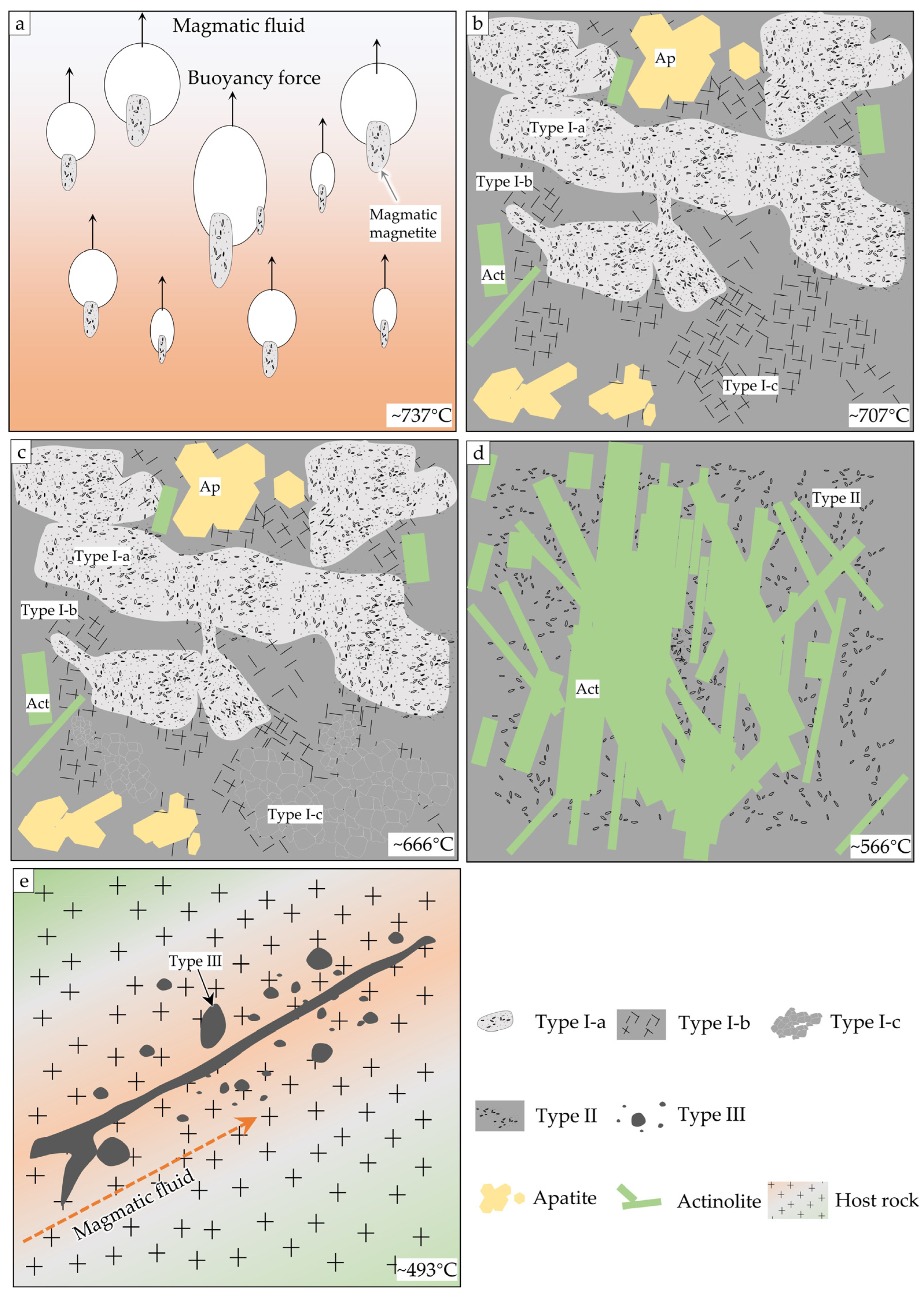
6.3. Magnetite Mineralization Process

The gradual contact between the ore and the host rock at the Mariela deposit is commonly interpreted as being formed by the hydrothermal process, which is widely accepted. However, the origin of the abrupt contact, where massive magnetite precipitates without significant alteration of the host rock, requires further consideration. In this study, massive magnetite (Type I/Type II) exhibits a potential magmatic origin, prompting the crucial inquiry of how this magnetite was effectively transported from the magma chamber following its initial crystallization. The “magnetite flotation model” proposed by Knipping [22,23] suggests that volatiles exsolved from the magma can form fluid bubble-magnetite pairs, which ascend due to buoyancy forces and accumulate at the top of the magma chamber. The successful transportation of magnetite out of the magma chamber necessitates a highly efficient fluid capable of carrying the magnetite, as otherwise it would tend to sink back into the magma chamber rather than form an ore deposit. Tectonic stress changes leading to regional extension and/or concentric faulting related to caldera subsidence might play a major role in separating the magmatic magnetite from the magma chamber through structural focusing [22,23,24]. The structural change likely causes a rapid decrease in magmatic fluid pressure, facilitating the transportation of early-stage magnetite. At Mariela, the presence of brecciated host rock in the massive ore suggests the involvement of high-pressure fluid movement during the mineralization process. In this context, it is plausible that the abrupt contact between the massive magnetite and the host rock can be attributed to the rapid deposition and accumulation of early-stage magnetite (Type I/Type II) facilitated by the magmatic fluid. Conversely, the gradual contact is likely a result of subsequent hydrothermal processes, leading to the formation of veined and disseminated magnetite (Type III).

In summary, the data presented in this study reflect the evolution of the Mariela deposit, which is characterized by several formation processes under different conditions that are documented by significant textural and chemical variations. Five steps of magnetite mineralization are recognized in this study (Figure 11).

(1)

The inclusion-rich Type I-a magnetite initially formed from magma or high-temperature magmatic-hydrothermal fluid, triggering bubble nucleation and forming a magnetite-fluid suspension (Figure 11a). The average formation temperature is around 737 °C. Subsequently, Type I-a magnetite was able to be transported by the fluid to shallow depths through a pre-existing regional fault trending NNW at Mariela.

(2)

As the high-temperature magmatic-hydrothermal fluid ascended and was transported to open spaces, the decompression would lead to a weakened capacity for magnetite transportation. Consequently, Type I-a magnetite began to precipitate, while inclusion-free Type I-b magnetite formed during the transportation process, with an average formation temperature of approximately 707 °C (Figure 11b).

(3)

The mosaic texture is displayed by Type I-c magnetite from Mariela, which is considered evidence of textural re-equilibration resulting from annealing and recrystallization of magnetite [58]. In particular, it can be formed through simultaneous recrystallization and annealing of inclusion-rich magnetite in IOCG and IOA deposits [29,56]. Moreover, a transitional relationship between Type I-b and Type I-c magnetite is supported by microscopic textures (Figure 4d). We interpret that at least a substantial proportion of Type I-c magnetite is the result of re-equilibration of Type I-b magnetite at an average formation temperature of approximately 666 °C (Figure 11c). Consequently, the Type I-a, I-b, and I-c magnetite, along with actinolite and apatite, constituted the most important high-grade massive ore at Mariela.

(4)

The hydrothermal fluid continued to migrate into the host rocks, and due to factors such as changes in fluid composition and temperature, a significant amount of Type II magnetite and actinolite crystallized, forming high-grade massive actinolite-magnetite ore (Figure 11d). The average formation temperature of approximately 566 °C suggests that this magnetite formed slightly after the Type I magnetite.

(5)

With the decrease in temperature, the fluid permeated the host rock through microfractures and formed veinlets or disseminated hydrothermal magnetite (Type III) at a relatively lower temperature of approximately 493 °C, accompanied by pervasive albitization alteration (Figure 11e).

7. Conclusions

The Mariela deposit is hosted in gabbro-dioritic intrusions, which are part of the Punta Coles Superunit. The iron ore bodies consist of massive and disseminated magnetite, actinolite, and apatite. Based on textural and chemical studies, including EPMA, LA-ICP-MS data, and SEM observations, three different types of magnetite are recognized at Mariela: Type I, representing the massive magnetite ore, which is sub-classified into inclusion-rich Type I-a, inclusion-free Type I-b, and mosaic Type I-c; Type II, characterized by the association with abundant actinolite and titanite; and Type III, representing the hydrothermally disseminated magnetite in strongly altered host rocks.

The geochemical discrimination diagrams show that the magnetite from Mariela formed in a magmatic-to-hydrothermal transitional environment. A discernible cooling trend is recognized, with successive decreases in temperature from the three subtypes (Type I-a, I-b, and I-c) of Type I magnetite to Type II and Type III magnetite. The highest average T_Mg-Mag temperatures were obtained in Type I-a magnetite (500–922 °C, avg. 737 °C), followed by Type I-b magnetite (418–837 °C, avg. 707 °C), and Type I-c magnetite (521–950 °C, avg. 666 °C). Type II and Type III magnetite formed at relatively lower temperatures (398–961 °C, avg. 566 °C; 423–558 °C, avg. 493 °C, respectively).

The micro-textures and geochemistry of magnetite presented in this study support the “magnetite-flotation model” [22,23]. The magmatic fluid transported magmatic or high-temperature magmatic-hydrothermal inclusion-rich magnetite into open spaces, where it precipitated as high-grade massive ore, along with inclusion-free or inclusion-poor magnetite subsequently formed from the cooling fluid. Overall, the ore-forming process in Mariela underwent a transition from magmatic to hydrothermal stages, covering a broad temperature range. Furthermore, no low-temperature magnetite was found in this study. Therefore, it is proposed that the Mariela deposit is a high-temperature magmatic-hydrothermal ore deposit, with temperatures ranging from approximately 500 to over 700 °C. The regional Mesozoic NNW-trending structure in the Costal Batholith may have served as an important trigger for final mineralization.

References

1. Williams, P.J.; Barton, M.D.; Johnson, D.A.; Fontboté, L.; De Haller, A.; Mark, G.; Oliver, N.H.S.; Marschik, R. Iron oxide copper-gold deposits: Geology, space-time distribution, and possible modes of origin. In Economic Geology 100th Anniversary Volume; Society of Economic Geologists: Littleton, CO, USA, 2005; pp. 371–405. [Google Scholar]
2. Sillitoe, R.H. Iron oxide-copper-gold deposits: An Andean view. Miner. Depos. 2003, 38, 787–812. [Google Scholar] [CrossRef]
3. Hou, T.; Charlier, B.; Holtz, F.; Veksler, I.; Zhang, Z.; Thomas, R.; Namur, O. Immiscible hydrous Fe-Ca-P melt and the origin of iron oxide-apatite ore deposits. Nat. Commun. 2018, 9, 1415. [Google Scholar] [CrossRef] [PubMed] [Green Version]
4. Nystroem, J.O.; Henriquez, F. Magmatic features of iron ores of the Kiruna type in Chile and Sweden; Ore textures and magnetite geochemistry. Econ. Geol. 1994, 89, 820–839. [Google Scholar] [CrossRef]
5. Chen, H.; Clark, A.H.; Kyser, T.K. The Marcona magnetite deposit, Ica, south-central Peru; A product of hydrous, iron oxide-rich melts? Econ. Geol. Bull. Soc. Econ. Geol. 2010, 105, 1441–1456. [Google Scholar] [CrossRef]
6. Velasco, F.; Tornos, F.; Hanchar, J.M. Immiscible iron-and silica-rich melts and magnetite geochemistry at the El Laco volcano (northern Chile): Evidence for a magmatic origin for the magnetite deposits. Ore Geol. Rev. 2016, 79, 346–366. [Google Scholar] [CrossRef]
7. Tornos, F.; Velasco, F.; Hanchar, J.M. Iron-rich melts, magmatic magnetite, and superheated hydrothermal systems: The El Laco deposit, Chile. Geology 2016, 44, 427–430. [Google Scholar] [CrossRef] [Green Version]
8. Sillitoe, R.H.; Burrows, D.R. New field evidence bearing on the origin of the El Laco magnetite deposit, northern Chile. Econ. Geol. 2002, 97, 1101–1109. [Google Scholar]
9. Barton, M.D.; Johnson, D.A. Evaporitic-source model for igneous-related fe oxide-(REE-Cu-Au-U) mineralization. Geology 1996, 24, 259–262. [Google Scholar] [CrossRef]
10. Rhodes, A.L.; Oreskes, N. Oxygen isotope composition of magnetite deposits at El Laco, Chile: Evidence of formation from isotopically heavy fluids. In Geology and Ore Deposits of the Central Andes; Society of Economic Geologists: Littleton, CO, USA, 1999. [Google Scholar]
11. Westhues, A.; Hanchar, J.M.; Lemessurier, M.J.; Whitehouse, M.J. Evidence for hydrothermal alteration and source regions for the Kiruna iron oxide-apatite ore (northern Sweden) from zircon hf and o isotopes. Geology 2017, 45, 571–574. [Google Scholar] [CrossRef]
12. Westhues, A.; Hanchar, J.M.; Whitehouse, M.J.; Martinsson, O. New constraints on the timing of host-rock emplacement, hydrothermal alteration, and iron oxide-apatite mineralization in the Kiruna district, norrbotten, sweden. Econ. Geol. 2016, 111, 1595–1618. [Google Scholar] [CrossRef]
13. Westhues, A.; Hanchar, J.M.; Voisey, C.R.; Whitehouse, M.J.; Rossman, G.R.; Wirth, R. Tracing the fluid evolution of the Kiruna iron oxide apatite deposits using zircon, monazite, and whole rock trace elements and isotopic studies. Chem. Geol. 2017, 466, 303–322. [Google Scholar] [CrossRef]
14. Dare, S.A.S.; Barnes, S.; Beaudoin, G.; Meric, J.; Boutroy, E.; Potvin-Doucet, C. Trace elements in magnetite as petrogenetic indicators. Miner. Depos. 2014, 49, 785–796. [Google Scholar] [CrossRef]
15. Nadoll, P.; Angerer, T.; Mauk, J.L.; French, D.; Walshe, J. The chemistry of hydrothermal magnetite: A review. Ore Geol. Rev. 2014, 61, 1–32. [Google Scholar] [CrossRef]
16. Palma, G.; Barra, F.; Reich, M.; Simon, A.C.; Romero, R. A review of magnetite geochemistry of Chilean iron oxide-apatite (IOA) deposits and its implications for ore-forming processes. Ore Geol. Rev. 2020, 126, 103748. [Google Scholar] [CrossRef]
17. Rojas, P.A.; Barra, F.; Deditius, A.; Reich, M.; Simon, A.; Roberts, M.; Rojo, M. New contributions to the understanding of Kiruna-type iron oxide-apatite deposits revealed by magnetite ore and gangue mineral geochemistry at the El Romeral deposit, Chile. Ore Geol. Rev. 2018, 93, 413–435. [Google Scholar] [CrossRef] [Green Version]
18. Salazar, E.; Barra, F.; Reich, M.; Simon, A.; Leisen, M.; Palma, G.; Romero, R.; Rojo, M. Trace element geochemistry of magnetite from the Cerro Negro Norte iron oxide-apatite deposit, northern Chile. Miner. Depos. 2020, 55, 409–428. [Google Scholar] [CrossRef]
19. Barnes, S.J.; Roeder, P.L. The range of spinel compositions in terrestrial mafic and ultramafic rocks. J. Petrol. 2001, 42, 2279–2302. [Google Scholar] [CrossRef]
20. Carew, M.J.; Mark, G.; Oliver, N.; Pearson, N. Trace element geochemistry of magnetite and pyrite in Fe oxide (cu? Au) mineralised systems: Insights into the geochemistry of ore-forming fluids. Geochim. Cosmochim. Acta 2006, 70, 5. [Google Scholar] [CrossRef]
21. Dupuis, C.; Beaudoin, G. Discriminant diagrams for iron oxide trace element fingerprinting of mineral deposit types. Miner. Depos. 2011, 46, 319–335. [Google Scholar] [CrossRef]
22. Knipping, J.L.; Bilenker, L.D.; Simon, A.C.; Reich, M.; Barra, F.; Deditius, A.P.; Lundstrom, C.; Bindeman, I.; Munizaga, R. Giant Kiruna-type deposits form by efficient flotation of magmatic magnetite suspensions. Geology 2015, 43, 591. [Google Scholar] [CrossRef] [Green Version]
23. Knipping, J.L.; Bilenker, L.D.; Simon, A.C.; Reich, M.; Barra, F.; Deditius, A.P.; Wälle, M.; Heinrich, C.A.; Holtz, F.; Munizaga, R. Trace elements in magnetite from massive iron oxide-apatite deposits indicate a combined formation by igneous and magmatic-hydrothermal processes. Geochim. Cosmochim. Acta 2015, 171, 15–38. [Google Scholar] [CrossRef] [Green Version]
24. Reich, M.; Simon, A.C.; Barra, F.; Palma, G.; Hou, T.; Bilenker, L.D. Formation of iron oxide-apatite deposits. Nat. Rev. Earth Environ. 2022, 3, 758–775. [Google Scholar] [CrossRef]
25. Reich, M.; Simon, A.C.; Deditius, A.; Barra, F.; Chryssoulis, S.; Lagas, G.; Tardani, D.; Knipping, J.; Bilenker, L.; Sánchez-Alfaro, P. Trace element signature of pyrite from the Los Colorados iron oxide-apatite (IOA) deposit, Chile: A missing link between Andean IOA and iron oxide copper-gold systems? Econ. Geol. 2016, 111, 743–761. [Google Scholar] [CrossRef] [Green Version]
26. Palma, G.; Reich, M.; Barra, F.; Ovalle, J.T.; Del Real, I.; Simon, A.C. Thermal evolution of Andean iron oxide-apatite (IOA) deposits as revealed by magnetite thermometry. Sci. Rep. 2021, 11, 18424. [Google Scholar] [CrossRef] [PubMed]
27. La Cruz, N.L.; Ovalle, J.T.; Simon, A.C.; Konecke, B.A.; Barra, F.; Reich, M.; Leisen, M.; Childress, T.M. The geochemistry of magnetite and apatite from the El Laco iron oxide-apatite deposit, Chile: Implications for ore genesis. Econ. Geol. 2020, 115, 1461–1491. [Google Scholar] [CrossRef]
28. Ovalle, J.T.; La Cruz, N.L.; Reich, M.; Barra, F.; Simon, A.C.; Konecke, B.A.; Rodriguez-Mustafa, M.A.; Deditius, A.P.; Childress, T.M.; Morata, D. Formation of massive iron deposits linked to explosive volcanic eruptions. Sci. Rep. 2018, 8, 14855. [Google Scholar] [CrossRef] [PubMed] [Green Version]
29. Ovalle, J.T.; Reich, M.; Barra, F.; Simon, A.C.; Deditius, A.P.; Le Vaillant, M.; Neill, O.K.; Palma, G.; Romero, R.; Román, N.; et al. Magmatic-hydrothermal evolution of the El Laco iron deposit revealed by trace element geochemistry and high-resolution chemical mapping of magnetite assemblages. Geochim. Cosmochim. Acta 2022, 330, 230–257. [Google Scholar] [CrossRef]
30. Instituto Geológico Minero y Metalúrgico. Peruvian Geological Map in Scale of 1:1,000,000, Edition: Cartografía Geológica Digital. Available online: https://portal.ingemmet.gob.pe/web/guest/carta-geologica-nacional (accessed on 13 April 2023). (In Spanish).
31. Data Basin. 30 Arc-Second Dem of South America. Available online: https://databasin.org/datasets/d8b7e23f724d46c99db1421623fd1b4f/ (accessed on 13 April 2023).
32. Esri. World Imagery [Basemap]. Available online: https://www.arcgis.com/home/item.html?id=c03a526d94704bfb839445e80de95495 (accessed on 3 April 2021).
33. Ramos, V.A. The basement of the central Andes: The Arequipa and related terranes. Annu. Rev. Earth Planet. Sci. 2008, 36, 289–324. [Google Scholar] [CrossRef]
34. Boekhout, F.; Spikings, R.; Sempere, T.; Chiaradia, M.; Ulianov, A.; Schaltegger, U. Mesozoic arc magmatism along the southern Peruvian margin during Gondwana breakup and dispersal. Lithos 2012, 146, 48–64. [Google Scholar] [CrossRef]
35. Cobbing, E.J.; Pitcher, W.S. The coastal batholith of central Peru. J. Geol. Soc. 1972, 128, 421–460. [Google Scholar] [CrossRef]
36. Demouy, S.; Paquette, J.; de Saint Blanquat, M.; Benoit, M.; Belousova, E.A.; O’Reilly, S.Y.; García, F.; Tejada, L.C.; Gallegos, R.; Sempere, T. Spatial and temporal evolution of Liassic to Paleocene arc activity in southern Peru unraveled by zircon U-Pb and hf in-situ data on plutonic rocks. Lithos 2012, 155, 183–200. [Google Scholar] [CrossRef] [Green Version]
37. Injoque, E.J. Fe oxide-cu-au deposits in Peru an integrated view. In Hydrothermal Iron Oxide Copper-Gold and Related Deposits: A Global Perspective; Porter, T., Ed.; PGC Publishing: Adelaide, Australia, 2002; Volume 2, pp. 97–113. [Google Scholar]
38. Shatwel, D. Mesozoic metallogenesis of Peru: A reality check on geodynamic models. SEG Discov. 2021, 124, 15–24. [Google Scholar] [CrossRef]
39. Cesar, E.V.C.; Jorge, I.-E.; Gary, B.S.; Samuel, B.M. Amphibolitic Cu-Fe skarn deposits in the central coast of Peru. Econ. Geol. 1990, 85, 1447–1461. [Google Scholar]
40. Benavides-Caceres, V.; Skinner, B.J. Orogenic evolution of the Peruvian Andes; The Andean cycle. Spec. Publ. (Soc. Econ. Geol. (U.S.)) 1999, 7, 61–107. [Google Scholar]
41. Chen, H.; Cooke, D.R.; Baker, M.J. Mesozoic iron oxide copper-gold mineralization in the central Andes and the Gondwana supercontinent breakup. Econ. Geol. 2013, 108, 37–44. [Google Scholar] [CrossRef] [Green Version]
42. Instituto Geológico Minero y Metalúrgico. Peruvian Geological Map in Scale of 1:50,000 Sheet 35-s Quadrant-1, Edition: Cartografía Geológica Digital. Available online: https://portal.ingemmet.gob.pe/web/guest/carta-geologica-nacional (accessed on 13 April 2023). (In Spanish).
43. Instituto Geológico Minero y Metalúrgico. Peruvian Geological Map in Scale of 1:50,000 Sheet 35-t Quadrant-4, Edition: Cartografía Geológica Digital. Available online: https://portal.ingemmet.gob.pe/web/guest/carta-geologica-nacional (accessed on 13 April 2023). (In Spanish).
44. Google Earth Pro 7.3.6.9345 (64-bit). 24 March 2021. Mariela, Arequipa, Eye Alt 5 km, CNES/Airbus. Available online: https://earth.google.com/web/@-17.10502921,-71.53617466,822.89918108a,5481.03498818d,35y,0h,0t,0r (accessed on 3 April 2021).
45. Yang, S.; Jiang, S.; Mao, Q.; Chen, Z.; Rao, C.; Li, X.; Li, W.; Yang, W.; He, P.; Li, X. Electron probe microanalysis in geosciences: Analytical procedures and recent advances. Atom. Spectrosc. 2022, 43, 186–200. [Google Scholar] [CrossRef]
46. Ning, S.Y.; Wang, F.Y.; Xue, W.D.; Zhou, T.F. Geochemistry of the Baoshan pluton in the Tongling region of the lower Vangtze river belt. Geochimica 2017, 46, 397–412, (In Chinese with English abstract). [Google Scholar]
47. Fangyue, W.; Gan, G.; Siyuan, N.; Liqing, N.; Guoxiong, Z.; White, N.C. A new approach to LA-ICP-MS mapping and application in geology. Acta Petrol. Sin. 2017, 33, 3422–3436. [Google Scholar]
48. Jochum, K.P.; Nohl, U.; Herwig, K.; Lammel, E.; Stoll, B.; Hofmann, A.W. Georem: A new geochemical database for reference materials and isotopic standards. Geostand. Geoanal. Res. 2005, 29, 333–338. [Google Scholar] [CrossRef]
49. Liu, Y.; Hu, Z.; Gao, S.; Günther, D.; Xu, J.; Gao, C.; Chen, H. In situ analysis of major and trace elements of anhydrous minerals by LA-ICP-MS without applying an internal standard. Chem. Geol. 2008, 257, 34–43. [Google Scholar] [CrossRef]
50. Klemm, D.D.; Henckel, J.; Dehm, R.M.; Von Gruenewaldt, G. The geochemistry of titanomagnetite in magnetite layers and their host rocks of the eastern bushveld complex. Econ. Geol. 1985, 80, 1075–1088. [Google Scholar] [CrossRef]
51. Nadoll, P.; Mauk, J.L.; Hayes, T.S.; Koenig, A.E.; Box, S.E. Geochemistry of magnetite from hydrothermal ore deposits and host rocks of the mesoproterozoic belt supergroup, United States. Econ. Geol. 2012, 107, 1275–1292. [Google Scholar] [CrossRef]
52. Nadoll, P.; Mauk, J.L.; Leveille, R.A.; Koenig, A.E. Geochemistry of magnetite from porphyry Cu and skarn deposits in the southwestern United States. Miner. Depos. 2015, 50, 493–515. [Google Scholar] [CrossRef]
53. Wen, G.; Li, J.W.; Hofstra, A.H.; Koenig, A.E.; Lowers, H.A.; Adams, D. Hydrothermal reequilibration of igneous magnetite in altered granitic plutons and its implications for magnetite classification schemes: Insights from the Handan-Xingtai iron district, north China craton. Geochim. Cosmochim. Acta 2017, 213, 255–270. [Google Scholar] [CrossRef]
54. Sievwright, R.H.; O Neill, H.S.C.; Tolley, J.; Wilkinson, J.J.; Berry, A.J. Diffusion and partition coefficients of minor and trace elements in magnetite as a function of oxygen fugacity at 1150 °C. Contrib. Mineral. Petrol. 2020, 175, 40. [Google Scholar] [CrossRef] [Green Version]
55. Deditius, A.P.; Reich, M.; Simon, A.C.; Suvorova, A.; Knipping, J.; Roberts, M.P.; Rubanov, S.; Dodd, A.; Saunders, M. Nanogeochemistry of hydrothermal magnetite. Contrib. Mineral. Petrol. 2018, 173, 46. [Google Scholar] [CrossRef]
56. Huang, X.; Beaudoin, G. Textures and chemical compositions of magnetite from iron oxide copper-gold (IOCG) and Kiruna-type iron oxide-apatite (IOA) deposits and their implications for ore genesis and magnetite classification schemes. Econ. Geol. 2019, 114, 953–979. [Google Scholar] [CrossRef]
57. Nold, J.L.; Davidson, P.; Dudley, M.A. The Pilot Knob magnetite deposit in the Proterozoic St. Francois mountains terrane, southeast Missouri, USA: A magmatic and hydrothermal replacement iron deposit. Ore Geol. Rev. 2013, 53, 446–469. [Google Scholar] [CrossRef]
58. Ciobanu, C.L.; Cook, N.J. Skarn textures and a case study: The Ocna de Fier-Dognecea orefield, Banat, Romania. Ore Geol. Rev. 2004, 24, 315–370. [Google Scholar] [CrossRef]
59. Hu, B.; Zeng, L.; Liao, W.; Wen, G.; Hu, H.; Li, M.Y.H.; Zhao, X. The origin and discrimination of high-Ti magnetite in magmatic-hydrothermal systems: Insight from machine learning analysis. Econ. Geol. 2022, 117, 1613–1627. [Google Scholar] [CrossRef]
60. Canil, D.; Lacourse, T. Geothermometry using minor and trace elements in igneous and hydrothermal magnetite. Chem. Geol. 2020, 541, 119576. [Google Scholar] [CrossRef]
Figure 1. Map showing the location of the Mariela IOA deposit within the Coastal Cordillera of Southern Peru. Jurassic and Cretaceous igneous rocks [30] and other ore deposits are also shown. Digital elevation model from Data Basin [31]. Background image in the Pacific Ocean area from Esri [32].
Minerals 13 00934 g001
Figure 2. Regional and local geological maps of Mariela. (a) A regional geology map showing the geological background of the Mariela deposit. Modified from Peruvian national geological maps [42,43]; (b) a geological map of the Mariela deposit interpreted based on field observations and a resource model. Background image from Google Earth [44].
Minerals 13 00934 g002
Figure 3. Mineral paragenesis chart for the Mariela deposit. M (massive); D (disseminated); V (veinlets); E (exsolution lamellae); I-a, I-b, I-c, II, and III (types of magnetite). I-a, I-b, and I-c collectively constitute Type I magnetite. The thickness of lines represents the abundance of minerals. Question marks indicate that the presence of the mineral is inferred.
Minerals 13 00934 g003
Figure 4. Representative backscattered electron (BSE) images (ad) and optical microscope photos (ei) of magnetite samples from Mariela. (a) Inclusion-rich magnetite (Type I-a) with inclusion-poor magnetite (Type I-b). (b) Inclusion-poor magnetite (Type I-b) with well-developed ilmenite exsolution lamellae, associated with apatite. (c) Inclusion-poor Type I-c magnetite with ilmenite exsolution lamellae, characterized by mosaic texture. (d) Type I-b transition to Type I-c magnetite. (e) Type II magnetite with abundant actinolite and Titanite under reflected light. (f) Type III magnetite associated with titanomagnetite under reflected light. See the Type III magnetite, partly replaced by hematite. (g) Strongly altered augite grains coexisting with disseminated hydrothermal magnetite (Type III). (h) Strongly altered augite grain. See the altered plagioclase grain in the top left corner. (i) Disseminated magnetite (Type III). (ad) are BSE images. Photomicrographs (gi) were taken at the same location on the slide but under plane-polarized light, cross-polarized light, and reflected light. Abbreviations: Mag (magnetite), Inc (mineral inclusion), Ilm (ilmenite), Titano-Mag (Titanomagnetite), Act (actinolite), Ap (apatite), Hem (hematite), Aug (augite), Plg (plagioclase), Ttn (titanite).
Minerals 13 00934 g004
Figure 5. WDS maps for selected elements in magnetite from the Mariela deposit. (a) Back-scattered electron image of magnetite. (bi) WDS maps of elements Al, Mg, Fe, V, Ti, Cr, Ce, and Sr. See actinolite in (a,b), and titanite in (f). The red square marks the WDS map area. Abbreviations: Act (actinolite), Ttn (titanite).
Minerals 13 00934 g005
Figure 6. Statistical summary of the important trace element concentrations (per type/subtype of magnetite) from Mariela determined by using LA-ICP-MS. Data in ppm. The thick bar for each element in the five types of magnetite represents the interquartile range (IQR), spanning from the first quartile (Q1; 25%) to the third quartile (Q3; 75%). The whiskers above and below the bar represent the data range within 1.5IQR, specifically from (Q1 − 1.5IQR) to (Q3 + 1.5IQR). Outliers are defined as data points that fall outside the range of 1.5IQR. The median line calculation includes outliers.
Minerals 13 00934 g006
Figure 7. The [Ti + V] vs. [Al + Mn] diagram [21]. Most of Types I-a, I-b, and I-c plot in the Fe-Ti, V, and porphyry fields. Type II shows a wide range of [Al + Mn] concentration. Most of the Type III plots are in the porphyry field. Chilean IOA deposits data are from Deditius et al. [55], Knipping et al. [22,23], Ovalle et al. [28], Palma et al. [16], and Rojas et al. [17].
Minerals 13 00934 g007
Figure 8. The Ti vs. V diagram. The data for Mariela plots mostly in or close to the igneous field. The igneous and hydrothermal fields are from Nadoll et al. [15]. Chilean IOA deposits data are from Deditius et al. [55], Knipping et al. [22,23], Ovalle et al. [28], Palma et al. [16], and Rojas et al. [17].
Minerals 13 00934 g008
Figure 9. The Fe vs. V/Ti diagram. The data for Mariela plots mostly in or close to the hydrothermal field. The igneous and hydrothermal fields are from Wen et al. [53]. Chilean IOA deposits data are from Deditius et al. [55], Knipping et al. [22,23], La Cruz et al. [27], Ovalle et al. [28], Palma et al. [16], and Rojas et al. [17].
Minerals 13 00934 g009
Figure 10. Calculated formation temperatures for the Mariela deposit show a discernible cooling trend from massive magmatic-hydrothermal magnetite (Types I and II) to disseminated hydrothermal magnetite (Type III). The thick bar for the temperature of the five types of magnetite represents the interquartile range (IQR), spanning from the first quartile (Q1; Min) to the third quartile (Q3; Max). The whiskers above and below the bar represent the data range within 1.5IQR, specifically from (Q1 − 1.5IQR) to (Q3 + 1.5IQR). Outliers, defined as data points that fall outside the range of 1.5IQR. are shown as “O”. The median line and mean calculation include outliers, and the mean values are shown as “X”.
Minerals 13 00934 g010
Figure 11. Schematic model for the formation process of magnetite in Mariela. (a) Crystallization of Type I-a inclusion-rich magnetite in magma or magmatic-hydrothermal fluid. (b) Precipitation of inclusion-free Type I-b over Type I-a magnetite. (c) Formation of Type I-c magnetite through re-equilibration of Type I-b magnetite. (d) Precipitation of Type II magnetite with abundant actinolite. (e) Formation of late veinlets and disseminated magnetite (Type III).
Minerals 13 00934 g011