CNN2D-SENet-Based Prospecting Prediction Method: A Case Study from the Cu Deposits in the Zhunuo Mineral Concentrate Area in Tibet

Abstract

Intelligent prospecting and prediction are important research foci in the field of mineral resource exploration. To solve the problem of the performance degradation of deep convolutional neural networks, enhancing the attention to target information and suppressing unnecessary feature information, this paper proposes a new prospecting prediction method based on a two-dimensional convolutional neural network (CNN2D). This method mainly uses known Cu deposits as the positive sample labels, adopts the sliding window method for data enhancement, and uses the window area as a unit to extract spatial variation features. It is important to supplement squeeze-and-excitation networks (SENets) to add an attention mechanism to the channel dimension, assign a weight value to each feature layer, and finally make prospecting predictions by matching the features of the known deposit window area and the features of the unknown window area. This method allows the neural network to focus on certain characteristic channels and realizes prospecting prediction in the case where there are few known deposits so that the deep learning method can be more effectively used for the prospecting prediction of mineralization. Based on geological data, geochemical exploration data of water system sediments, and aeromagnetic data, and via this method, this study carried out prospecting prediction of Cu deposits in the Zhunuo area of Tibet and predicted 12 favorable Cu prospecting prediction areas. Combined with previous research results and field exploration, the predicted result is consistent with the established mineralization and prospecting pattern and has good prospects for Cu deposit prospecting.

1. Introduction

In recent years, deep learning has been used to help solve geoscience research problems [1,2,3,4,5]. For example, the use of deep learning to solve the problem of mineral prediction will help researchers overcome the difficulty of not fully considering geological variables and evaluating the reliability of the current model in the existing data [6,7,8,9].

At present, many studies have been carried out on prospecting prediction using unsupervised deep learning methods. For example, self-encoding networks are used to identify multiple geochemical anomalies and delineate prospecting areas [10,11,12], and self-organizing neural networks are used to cluster geological, geophysical and geochemical data and map mineral potential [13,14]. However, there are few studies on ore prospecting prediction using supervised neural networks.

Convolutional neural networks (CNNs), one of the most comprehensive neural networks developed to date, can perform representation learning; that is, they can extract high-order features from input information and at the same time can identify similar features located in different spatial locations [15]. At present, there are relatively mature applications in lithology identification [5] and high-resolution geological mapping [16] in geology. In recent years, Chinese and foreign scholars have successfully applied convolutional neural networks to prospecting and prediction research. Liu et al. [17] applied a convolutional neural network to establish a model of the relationship between surface Pb distribution characteristics and ore body placement in the Zhaojikou lead–zinc deposit in Anhui Province and carried out metallogenic prediction. They concluded that the convolutional neural network can effectively mine the relationship between the distribution of surface elements and the spatial relationship of the ore body in place. Li et al. [18] proposed a text mining method based on CNN classification and established a workflow for extracting key prospecting information from geoscience text data. Taking the Lala Cu deposits in Sichuan as an example, they completed intelligent classification and labeling, explored the potential relationship between the data, and realized the intelligent extraction of geological prospecting information. Cai et al. [2] took the Daqiao gold deposit in Gansu Province as an example and proposed the use of one-dimensional convolutional neural networks to replace traditional manual calculations to mine the comprehensive metallogenic information. According to the training results, metallogenic prospects were finally divided into four types, and the convolutional neural network model effectively realized the intelligent prediction and evaluation of mineral resources. Li et al. [10] used a CNN to map mineral prospects in southwestern Fujian Province, China. The mineral prospect areas obtained by the constructed model have strong spatial correlation with known mineralization locations; Li et al. [19] used geochemical data as training data, introduced transfer learning to train convolutional neural networks, and finally delineated a gold prospecting area in Zhangbaling, eastern Anhui Province, China.

Essentially, convolution is the feature fusion of a local region [20,21,22]. The attention mechanism is a special structure embedded in machine learning models to automatically learn and calculate the contribution of input data to output data [23]. The attention mechanism can filter out important information from a large amount of information. The SE attention mechanism of squeeze-and-excitation networks (SENets) is part of the channel attention mechanism and can adaptively learn the dependencies between different channels. Its main idea is to automatically learn the feature weights according to the loss, instead of directly evaluating according to the numerical distribution of the feature channel. This can make the weight of the effective feature channel larger, and the neural network can focus on the important feature channel [24]. The channel of the feature map that is useful for the current task is improved, and the feature channel that is not useful for the current task is suppressed, thereby increasing the accuracy of prediction to a certain extent.

In summary, to solve the problem of insufficient data volume of deep learning and improve the prediction accuracy, this paper proposes a method for intelligent prospecting prediction based on SENet-CNN2D. The dataset is obtained using the method of data enhancement, which overcomes the problem of insufficient training data to a certain extent. Taking the window as the analytical unit, the convolutional neural network is used to extract the anomalous spatial features of geological, geochemical, and geophysical data, and the channel weight is calculated by SENet. After channel weighting, by intelligently matching the data characteristics of known deposits and the data characteristics of the unknown window area, supervised deep learning prospecting prediction is realized, and Cu deposit prospecting experiments are carried out in the Zhunuo Cu deposits area in Tibet.

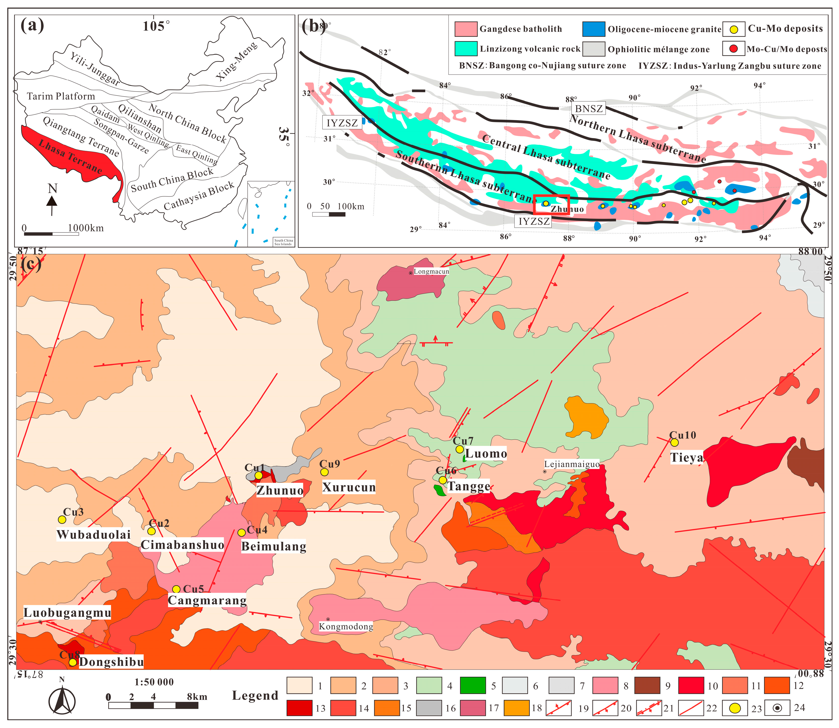
2. Regional Geological Background

The Zhunuo area of Tibet is located in the southern part of the Bangong Lake–Nujiang suture in the southern Qinghai–Tibet Plateau and the western part of the southern Lhasa Terrane to the north of the Yarlung Zangbo suture (Figure 1a,b) [25,26]. The exposed strata in the area are mainly the Jurassic–Lower Cretaceous Sangri Group (including the Mamuxia Group and Bima Group) and two sets of volcanic–sedimentary rock assemblages in the Paleogene Linzizong Group (including the Dianzhong Group, Nianbo Group, and Pana Group) [27,28,29]. Since the Jurassic, the study area has experienced the subduction of the Neo-Tethys oceanic crust, the convergence and collisional orogeny of the Indo-Asia continent, and the postcollisional intraplate process, and the associated magmatic activity is very strong. In particular, the strong intermediate–acid magmatism and tectonic action in the Himalayan period provided a good material source and transport and storage space for the formation of Cu-polymetallic deposits in this area, with good metallogenic geological conditions and prospecting prospects [30,31,32,33,34].

The magmatic rocks in the study area are widely distributed, with various rock types of Paleocene, Eocene, and Miocene ages. The main lithologies are porphyry-like monzonite granite, monzonite granite (porphyry), quartz porphyry, quartz monzonite diorite, potassium feldspar granite, granodiorite, etc. Among them, Miocene porphyritic monzogranite and monzogranite porphyry are closely related to mineralization [32,33,34].

The structure in the area distributes and accommodates magma and ore-bearing fluids, and it specifically controls mineralization through structural components, such as faults, fissures, and contact surfaces. Fault structures are relatively developed in the study area; NE-trending faults and NNE-trending faults are the most developed, especially NE-trending fault structures, which are the main rock- and ore-controlling structures [30,32,34]. Dense zones where multiple groups of primary dense faults and structural fissures intersect are favorable for ore blending and mineral precipitation enrichment. On both sides of the porphyry contact between the inside and outside, the faults are developed, the extension is large, and the source of ore liquid is abundant, which controls the spatial distribution of the mineralized and enriched section and the morphological characteristics of the deposit. Tectonic activity in the mining area is an important driving force for the emplacement of ore-bearing magma and the migration of ore-bearing hydrothermal fluids.

The Zhunuo Cu deposit is a typical orogenic porphyry Cu deposit formed in a postcollisional environment, and the metallogenic period was the late Himalayan [16,34]. Its formation was controlled by the following three factors. (1) The complex rock mass developed during the metallogenic period, and the complex rock mass intruded multiple times, thereby replenishing fluid and mineral and thermal energy multiple times. The longer the emplacement time lasts, the more favorable it is for the formation of large deposits, among which Miocene granites are the most direct ore-forming geological bodies. (2) The Miocene mantle-derived ultrapotassic–potassic magma is replenished by water injection, and the enclaves, lamprophyre, and high-magnesium diorite formed by mantle-derived magma are very important for the mineralization of the Zhunuo Cu deposit. (3) The NE-trending and nearly E–W-trending faults and fissures in the rock are the main regional metallogenic structures.

3. Methods

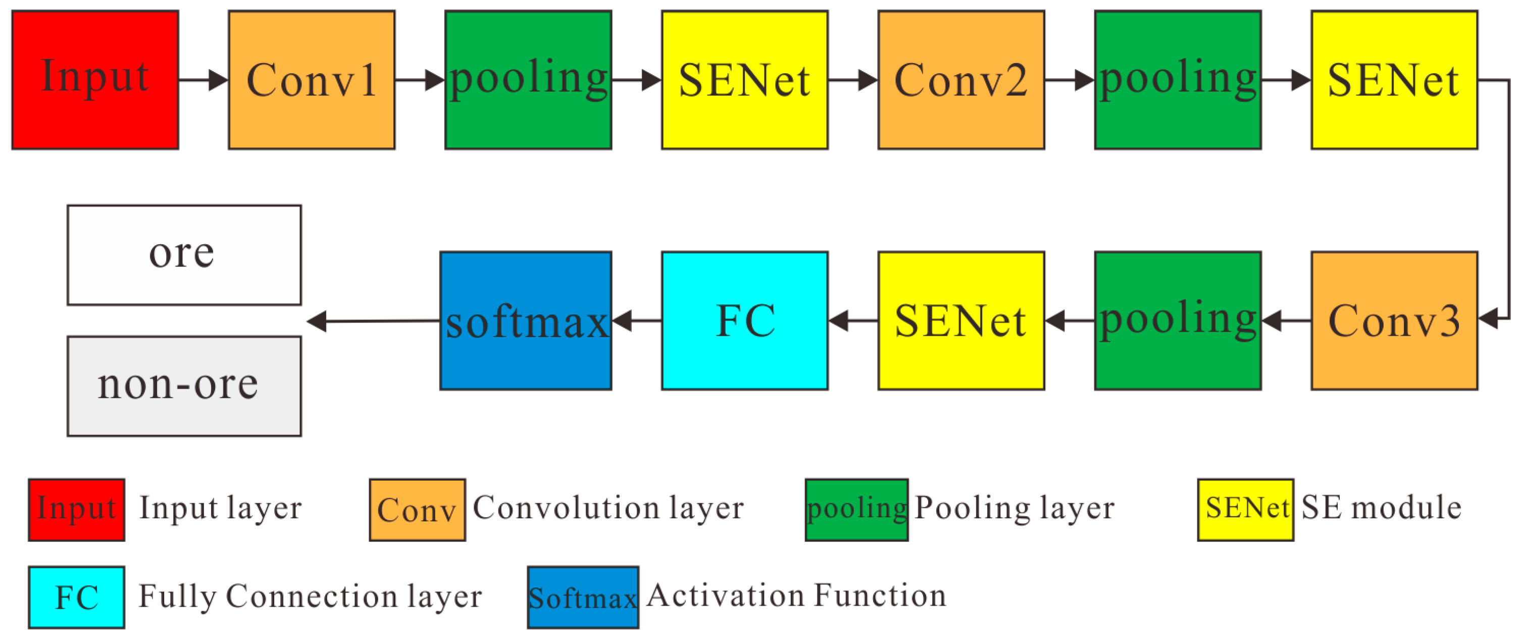
3.1. CNN2D-SENet Model

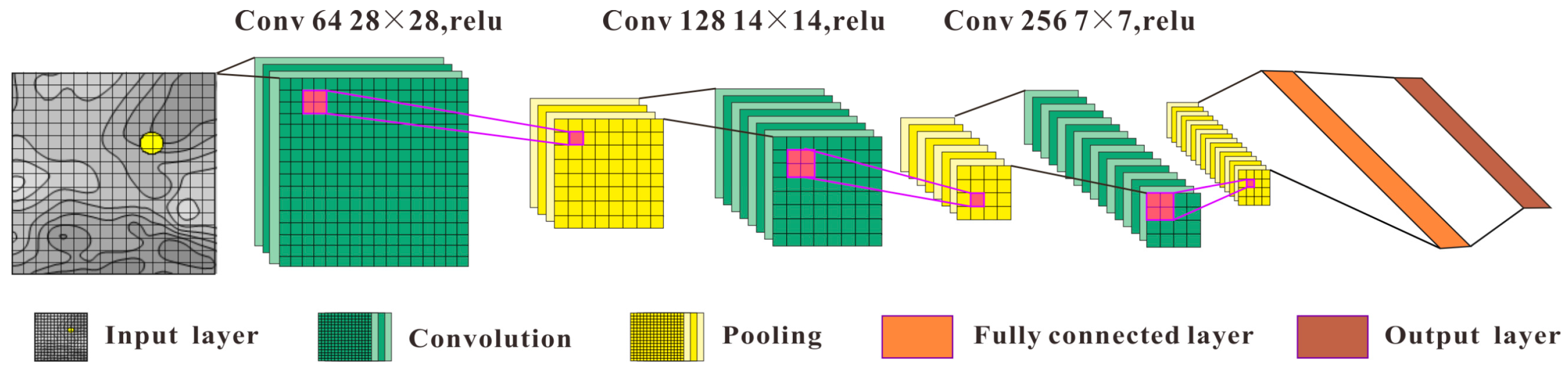
In this paper, the CNN2D-SENet model is used for prospecting prediction research, as shown in Figure 2. The model mainly consists of 3 convolution blocks, 3 pooling layers, 3 SE modules, and 2 fully connected layers. The implementation process of the algorithm is as follows. First, the original data can be directly input, and the feature information of the image is extracted by the two-dimensional convolution operation of the CNN2D network, which effectively avoids the complex feature design and preprocessing process in the traditional manual feature extraction method and saves time. Second, the dataset is expanded by the sliding window method to enhance the generalization ability of the network; then, to further improve the prediction accuracy, SENet is embedded in CNN2D, and finally, softmax is used to output the prediction result.

3.1.1. CNN2D

CNNs can not only simulate the processing mechanism of layer-by-layer feature extraction in the human visual system to extract the deeper features of the image, but it can also use the end-to-end feature extraction method, so that the extracted features have a strong generalization ability, avoiding the problem of inaccurate feature extraction caused by image transformation. The strength of CNNs lies in the well-designed architecture that is capable of extracting both local and global features of the input data [37].

The data input layer writes gridded input data into neural units. The convolutional layer and the pooling layer select the appropriate activation function to complete the extraction and sampling of the data features, respectively. The fully connected layer implements feature mapping and classification at the end of the network, and the feature output layer can be used for result output or feature visualization. Therefore, determining the appropriate convolutional layer and fully connected layer structure is crucial to the performance of the convolutional neural network model.

The CNN model used in this paper consists of 3 convolutional layers, 3 pooling layers, and 1 fully connected layer (Figure 3).

The role of the convolutional layer is to extract the features of the data matrix [38]. The input data matrix is processed by the convolution kernel so that a new data matrix (feature map) can be obtained. Then, the data features of different positions are extracted by sliding the window. Equation (1) is used to realize the convolution operation:

$$y=sig({\sum }_{p=0}^{P_{i-1}}{\sum }_{q=0}^{Q_{j-1}}\left(w_{p,q}{s}_{p,q}+b_{p,q}\right))$$

(1)

where s represents the input data, $w_{p,q}$ represents the weight,$b_{p,q}$ represents the bias vector, $sig\left(*\right)$ represents the activation function, $y$ represents the output data, and $P\times Q$ represents the size of the convolution kernel. After the image undergoes the convolution operation, its size is reduced accordingly with the size of the convolution kernel. To avoid changing its size, the same padding is usually used after convolution to restore the size of the feature map.

The pooling layer is used to compress the input feature data, simplify the network’s computational complexity, extract the main features, and control overfitting to a certain extent [39]. After the feature map is pooled, the size of the feature map decreases, but the original features still exist. This article uses max pooling. The pooling operation is implemented using Equation (2):

$$f{\left(x\right)}_j=\underset{i\in R_j}{\max }\left(x_i\right)$$

(2)

where $R_j$ is the $j$th region in the feature map $x$, and $i$ is the feature value in the $j$th region.

Through multiple convolution and pooling layers, the features extracted by the network model are dimensionally reduced. Finally, by establishing a fully connected layer, the feature matrix is expanded into a one-dimensional vector and then mapped to the classification sample space to obtain the probability value of the input data in each classification. The index value with the highest probability is the current classification. The fully connected operation is represented by Equation (3):

$$f{\left(x\right)}_i={\sum }_{j=0}^{W\times H\times C-1}\left(\left(w_{ij}\times x_i\right)+b_i\right)$$

(3)

where $W, H, \mathrm{and} C$ are the width, height, and number of channels of the input feature map; $w$ is the weight; $b$ is the bias vector; and $i$ is the ith value of the one-dimensional vector output by the fully connected layer.

After completing the above convolution and full connection operations, the output features are activated by executing the Rectified Linear Unit (ReLU) function, the positive value of the calculation result is retained, and the negative value is set to 0 to avoid overfitting during the training process.

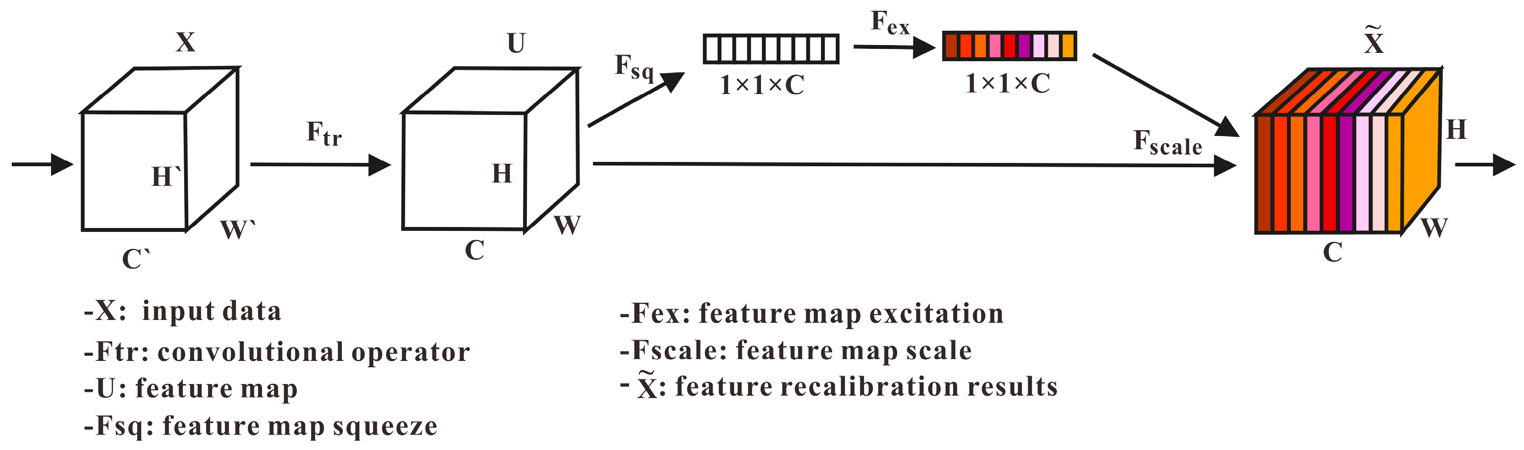
3.1.2. Squeeze-and-Excitation Network

An innovation of this paper is to introduce the SENet algorithm and embed it into CNN2D for prospecting prediction research. SENet mainly consists of squeeze and excitation. It uses a global average pooling-FC (fully connected)-ReLU-FC-Sigmoid method. SENet has two fully connected layers, and the roles of the two layers are opposite. Its principle is shown in Figure 4.

The main idea of SENet is to start from the relationship between feature maps, that is, to build a model based on the relationship between feature channels. The key point is that SENet can learn the importance of feature channels by itself, increase the weight of useful features, and reduce the weight of low-importance and useless features according to the importance of features [24]. In earlier layers of the network, it excites the features in a class-independent manner, enhancing the shared underlying representation. In the deeper and later layers of the network, SENet gradually becomes increasingly directional, and the dot product size of the later layers is strongly correlated with the input category. SENet is mainly composed of pooling layers, fully connected layers, and ReLU.

In essence, SENet performs an operation similar to the attention mechanism in the feature channel, where the input of SENet is the output of CNN2D. In the squeeze part, global average pooling (Equation (4)) is used to average the information of all points in space into one value. This is because the final scale is applied to the entire channel, and the scale must be calculated based on the overall information of the channel. In addition, the correlation between channels should be used, not the correlation in the spatial distribution. Using global average pooling to mask the spatial distribution information can make the calculation of scale more accurate. Formally, a statistic $\mathrm{z}\in R^C$ is generated by shrinking U through spatial dimensions H × W, where the c-th element of z is calculated by

$${\mathrm{z}}_c=F_{sq}\left(u_c\right)=\frac{1}{H\times W}{\sum }_{i=1}^H{\sum }_{j=1}^W{u}_c\left(i,j\right)$$

(4)

where u is the input feature, H × W represents the size of the spatial domain, and C is the channel dimension, $F_{sq}$ is the feature map squeeze.

After another operation is needed to learn the interdependence between the feature channels, namely, the excitation operation [24], as shown in Equation (5):

$$S=F_{ex}\left(z,w\right)=\sigma \left(g\left(z,w\right)\right)=\sigma (w_2\delta \left(w_{1}z\right)$$

(5)

where $w_1*$ and $w_2*$ represent the fully connected (FC) operation, $w_1$ is the dimension reduction parameter, $w_2$ is the dimension increase parameter, δ is the ReLU function, 𝜎 is the sigmoid function, and $F_{ex}$ is the feature map excitation.

The model uses two fully connected layers, which can also be understood as a 1*1 convolutional layer. Through a fully connected layer, the data dimension is reduced to C/r (r is the dimensionality reduction ratio) to reduce the amount of calculation. Then, a ReLU activation function, followed by a fully connected layer with a parameter of $w_2$, is used to improve the data dimension, which can solve some linear problems, strengthen the correlation between fitting channels, reduce the number of parameters, and simplify the tedious calculation process. That is, reducing the dimension first and then increasing the dimension can reduce the complexity of the model and play a role in assisting generalization. Finally, the sigmoid function is used to normalize the weights.

Finally, recalibration is performed to assign corresponding weights to each feature channel. The input is the original feature map, $u_c$, and the weight vector is $s_c$. The final output is the feature map $\widetilde{x_c}$, which is obtained by channel multiplication [24], as shown in Equation (6):

$$\widetilde{x_c}=F_{scale}\left(u_c,s_c\right)=s_c{u}_c$$

(6)

where $\tilde{X}=\left[\widetilde{x_1},\widetilde{x_2},\dots ,\widetilde{x_C}\right]$ and $F_{scale}\left(u_c,s_c\right)$ refers to channel-wise multiplication between the feature map $u_c\in R^{H\times W}$ and the scalar $s_c$.

In general, the SENet model can adaptively select important feature channels according to the global information of feature channels and reduce the selection of invalid feature channels.

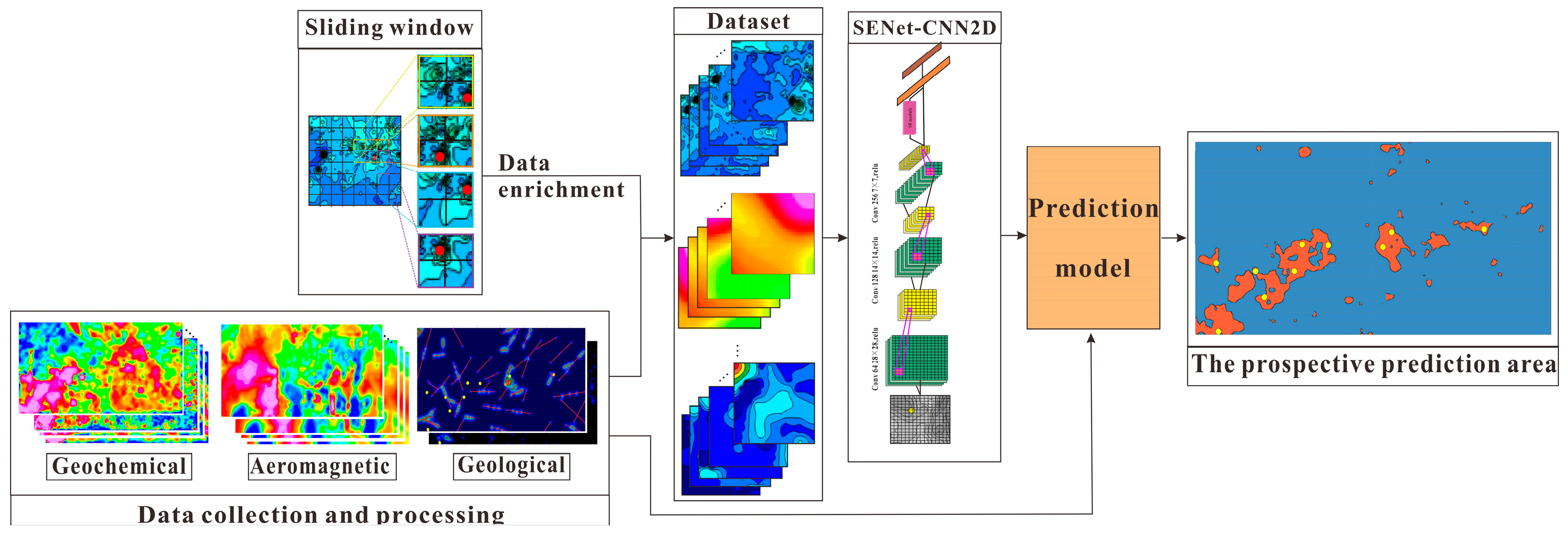
3.2. Method and Steps of Prospecting Prediction Based on the CNN2D-SENet Model

The prospecting prediction method based on the CNN2D-SENet model mainly uses known deposits as the type of prospecting prediction. The neural network is applied to the data grid of each dimension, the window sliding method is used [40,41] to extract the data features of all windows, and data augmentation techniques are used to obtain the training dataset and validation dataset. Here, the window is treated as an image. By learning the characteristics of spatial variation within the window area of known deposits, a prospecting prediction model is generated. In the ore prospecting prediction stage, the characteristics of each prospecting window are matched with the characteristics of the known ore deposits, and the window with a larger matching probability with the known ore deposits may have ore.

Prospecting prediction based on the CNN2D-SENet model includes the following steps (Figure 5).

(1)

Data preparation and processing

The regional geological survey spatial database and geochemical and aeromagnetic survey data were collected in the study area. In order to utilize all the data, the geological, geochemical, and aeromagnetic data were gridded mainly by kriging, and the original sparse and irregularly distributed data were interpolated into new regularly distributed data. The size of the grid cells depends on the scale of data collection.

(2)

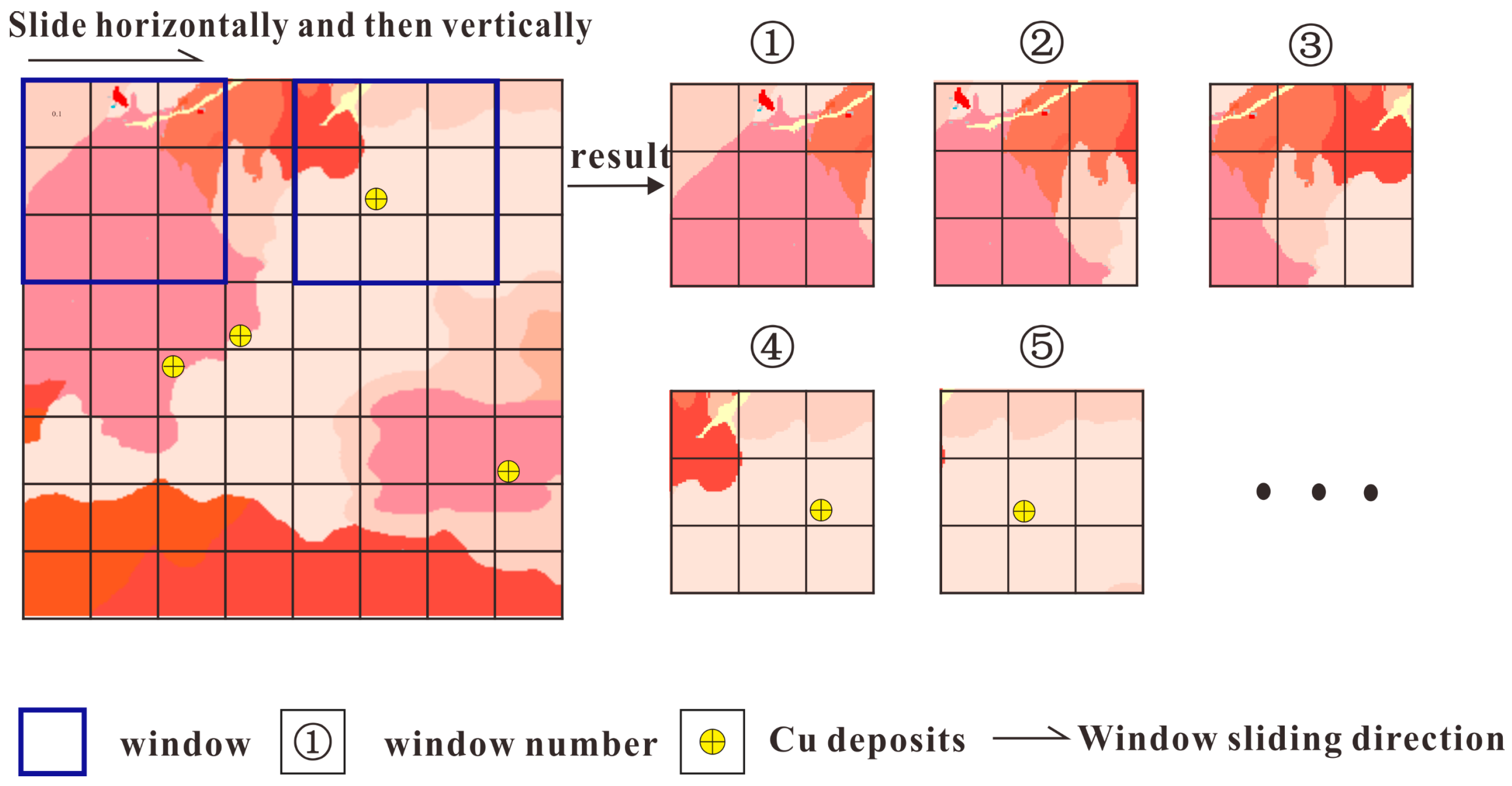
Construction of the training sample dataset

Generally, there are only a few to a dozen known deposits in a prediction area, and it is difficult to generate an effective prediction model only by training deep learning networks with these deposits. This paper uses the window-sliding data-enhancement method [37] to construct a training sample set to obtain a network with stronger generalization ability, which makes the results more convincing.

The window sliding data enhancement method adopts a certain window size, such as setting the window size to 14 grid units × 14 grid units. If there are n known deposits, n × 14 × 14 positive samples can be obtained through the sliding window (Figure 6, windows containing known deposits and mineral occurrences are considered known deposit labels and are called positive samples).

In areas far from known deposits and mineral occurrences, random sampling is performed to form m unknown deposits. Using the same window sliding method as the positive samples, m × 14 × 14 training data of negative samples were obtained (windows containing unknown deposits form labels of unknown deposits, called “negative samples”).

(3)

Construction of the CNN2D-SENet model

The prediction area is divided into a series of windows. Spatial feature data, such as geologic, geochemical, and aeromagnetic data, are collected for each window unit, and the convolutional neural network layer is used to automatically extract spatial structural features. According to the relationship between known deposits and types, favorable prospective areas are determined.

During learning, the positive and negative samples are mixed, and the order is shuffled and divided randomly to form a training dataset, of which 80% of the sample data are used for model training and 20% are used for model validation.

(4)

Generating prediction models and model training and verification

First, the model is trained and verified with the prepared training dataset; then, the model is trained with different parameters and hyperparameters, and the optimal model is selected through the verification set. The prediction area grid is predicted using the sliding window method, and the favorable prediction area is delineated. Here, the step size of the sliding window can be set to 1, 2, …, n. Finally, according to the mineral geological data, the reliability of the prediction results is analyzed to further determine the prospecting prediction area.

4. Application and Experiment

To verify the prediction effect of the CNN2D- SENet prospecting prediction model, we selected the Zhunuo area of Tibet, China, which has complete data and a high degree of research on it, such as mineral prospectivity mapping. The specific process is as follows.

4.1. Data and Data Processing

4.1.1. Geological Data

Mineral geological survey work at a 1:50,000 scale was systematically carried out in the study area, covering an area of 1635 km², with complete geological data and mineral geological survey data.

The influence of various geological features on mineralization decreases with the increase in the distance from the ground feature, so the function of distance can be used to express the intensity of the influence of geological elements on mineralization, as well as the relationship between various geological elements and mineralization. This is described here by the exponential function in Equation (7). Different attenuation coefficients can be used for different geological elements. The geological features considered are mainly faults, geological bodies, and geological boundaries.

$$I=a{e}^{-bx}$$

(7)

where a and b are the coefficients; a represents the magnitude of the impact (usually a = 1.0); b represents the attenuation coefficient, with a larger value representing faster attenuation (usually b = 0.01); x represents the distance from the geological element; and I represent the intensity of the impact.

Taking the calculation of the fault influence strength as an example, and assuming that there are n faults (F₁, F₂, …, F_n) in the study area, we select one of the faults Fi to obtain the shortest distance from each grid unit of the grid in the study area to the fault. According to the influence intensity calculation model, the influence intensity of the fault on each grid unit is calculated separately, and the influence intensity data layer GF_i corresponding to the fault Fi is obtained. By performing the above calculations for each fault in the study area, the fault impact data set represented by n data layers can be obtained. Similarly, if the influence strength of a geological body on mineralization is calculated, it can be calculated by obtaining the shortest distance from each grid unit to the boundary of the geological body. The influence intensity of grid cells inside the geological body takes a positive value, and the influence intensity of grid cells outside the geological body takes a negative value [42].

(1) Relationship between the influence intensity of the geological boundary and Cu deposits and mineral occurrences

Three high-influence intensity areas are present along the central and southwestern parts of the study area. The high-influence intensity areas are generally oriented in a northeast direction. The rest of the locations are medium- to low-value regions (Figure 7a). Most Cu deposits and mineral occurrences are located near the mid- to high-impact intensity area, and only Cu3 has low background values. It can be inferred that there is a great possibility of prospecting in the mid- to high-value contour area of the geological boundary.

(2) Relationship between the fault structure and Cu deposits and mineral occurrences

The influence intensity map of the fault structure (Figure 7b) shows that the NE and NW fault structures are mainly developed. Most Cu deposits and mineral occurrences are developed at the intersection of faults and near the high-value area, and Cu6, Cu7, and Cu10 are in the high-value area.

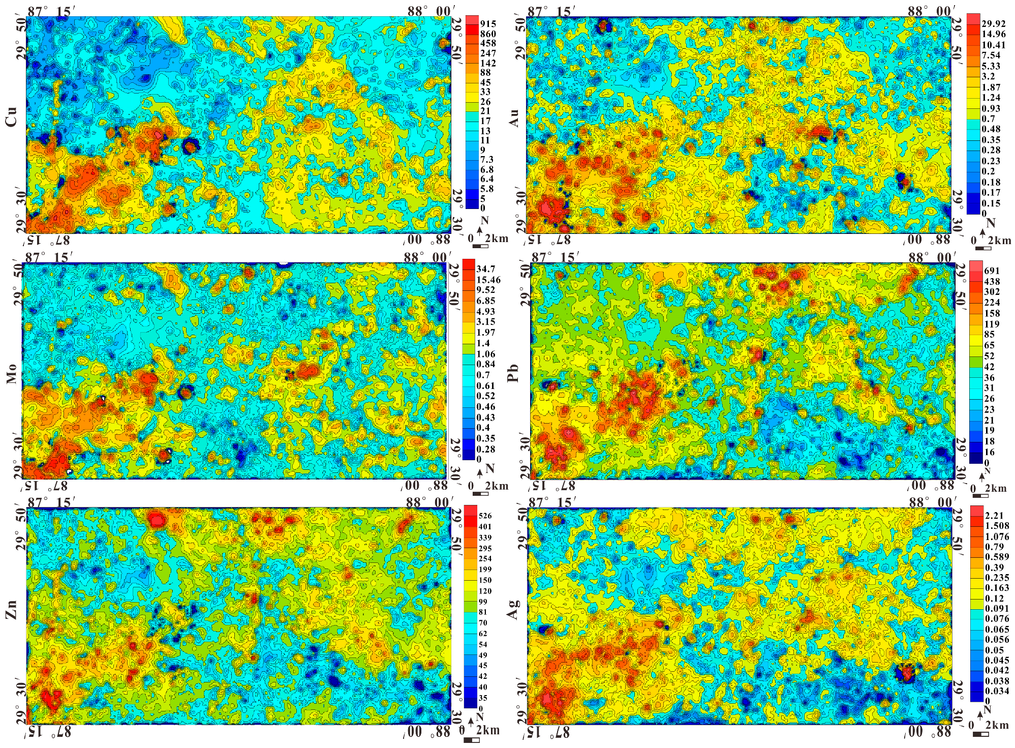
4.1.2. Geochemical Data

The study area has Ag, Au, Cu, Mo, Pb, and Zn elemental water sedimentary geochemical data from exploration. In this paper, the kriging interpolation method is used, the grid cell size is 50 m × 50 m (

Table 1. Grid criteria of geochemical element data.

Coordinates	Minimum/m	Maximum/m	Spacing/m	Unit Number
X direction	524177	596768	50	1453
Y direction	3,264,867.5	3,302,083.5	50	745

), the gridded data of six kinds of elements are obtained, and the grid cell is 1453 (rows) × 745 (columns) = 145,112 (units).

As shown in Figure 8, the main metallogenic elements, Cu, Mo, Au, Pb, Zn, and Ag, in the area have NE–SW distribution characteristics, and the concentration centers are well fitted. The southwestern corner of the study area is the key prospecting block. In general, the distribution of Cu and Mo elements in the study area is well matched, and most of them are distributed around the Miocene geological body. Au, Ag, Pb, and Zn are abnormally distributed in the periphery of Cu and Mo, which have transitional characteristics from high-temperature Cu and Mo to medium- and low-temperature Au, Ag, Pb, and Zn from inner to outer elements. The distribution characteristics of such elements indicate that the study area developed a porphyry epi-low-temperature hydrothermal metallogenic system; that is, porphyry Cu–Mo deposits should be found around the Miocene porphyry body during prospecting and exploration.

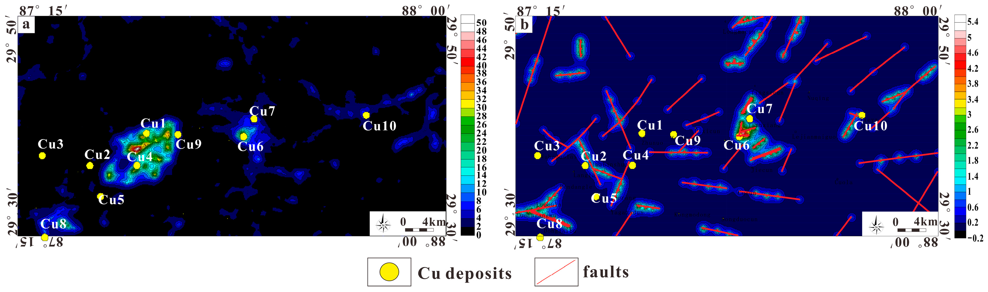
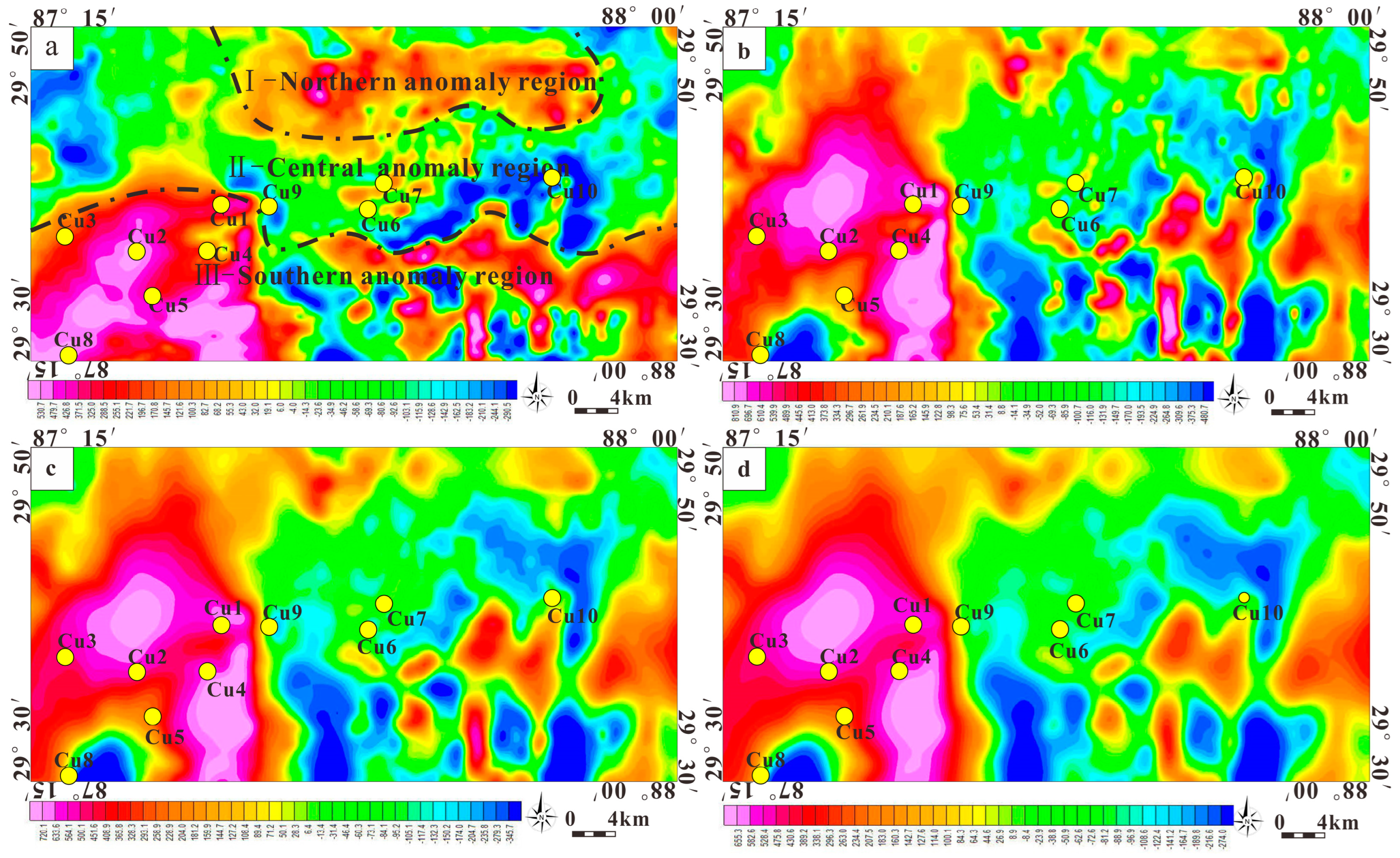
4.1.3. Geophysical Data

Airborne magnetic surveys were carried out, and the average spacing of the data sampling points was 250 m. Data were gridded to a grid cell size of 50 m × 50 m (same as Table 1; Figure 9a). Processing aeromagnetic data through polarization means transforming the abnormality of oblique magnetization into vertical magnetization (to the geomagnetic pole) and eliminating the asymmetry of magnetic anomalies caused by the inclination and declination of the magnetization field. On this basis, the upward continuation is carried out, and the results of 500 m upward (Figure 9c) and 1000 m (Figure 9d) upward are obtained.

There are two main high magnetic anomaly zones and one low anomaly zone (Figure 9a), which are the northern strong magnetic anomaly area, the central negative magnetic anomaly area, and the southern strong magnetic anomaly area. (1) The northern strong magnetic anomaly area is oriented in a nearly east–west direction. It is inferred that the intrusive rock mass is the magnetic source body formed by the magnetic anomaly in this area, and a NW-trending fault is present in the area. Structural–magmatic activities not only provide abundant metallogenic materials for mineralization but also provide good ore transport and ore storage space for the positioning and enrichment of ore deposits. (2) The central negative magnetic anomaly area is distributed in a nearly east–west direction. According to the statistical results of the measured physical properties, it is believed that the concealed and semi-concealed intrusive rocks (granite porphyry, monzogranite, and granodiorite) are the magnetic source bodies formed by the local magnetic anomalies in this area. The belt has good prospecting prospects, and the geological, magnetic, and geochemical anomalies fit well. (3) The southern strongly magnetic anomaly area is oriented in a nearly east–west direction. In most sections of the outcropping boundary of the rock mass, there are local anomalies in a beaded arrangement, indicating that the magnetic field characteristics in this area are well fitted with the geological conditions. Monzogranite and granodiorite are the main reasons for the anomaly in this area.

In this paper, the upward continuation method is used for research. The shallower disturbance is suppressed by the upward continuation, which suppresses the deep larger magnetic geological bodies to increase the information for interpreting inferences.

4.1.4. Deposits and Mineral Occurrence Data

There are 10 known Cu deposits and mineral occurrences in the study area (

Table 2. Known deposits and ore occurrences in the Zhunuo mineral concentration area.

Serial Number	Type	Size of the Deposit
Cu1	porphyry type	large
Cu2	porphyry type	ore occurrence
Cu3	porphyry type	ore occurrence
Cu4	porphyry type	ore occurrence
Cu5	porphyry type	ore occurrence
Cu6	skarn type	ore occurrence
Cu7	porphyry type	ore occurrence
Cu8	porphyry type	ore occurrence
Cu9	porphyry type	ore occurrence
Cu10	porphyry type	ore occurrence

). Through comparative analysis, the types of mineralization in the study area are found to include the following. (1) Porphyry-type Cu–Mo mineralization: the key ore-forming geological body is the Miocene porphyry body; the lithology is porphyry monzogranite, monzogranite porphyry or granite porphyry; and the rock mass is strongly altered. (2) Skarn-type Cu–Fe mineralization: the mineralization occurs in the skarn and skarnized limestone of the Bima Group, and the rock mass of this type of deposit is not developed.

4.2. Prediction Parameters and Prediction Results

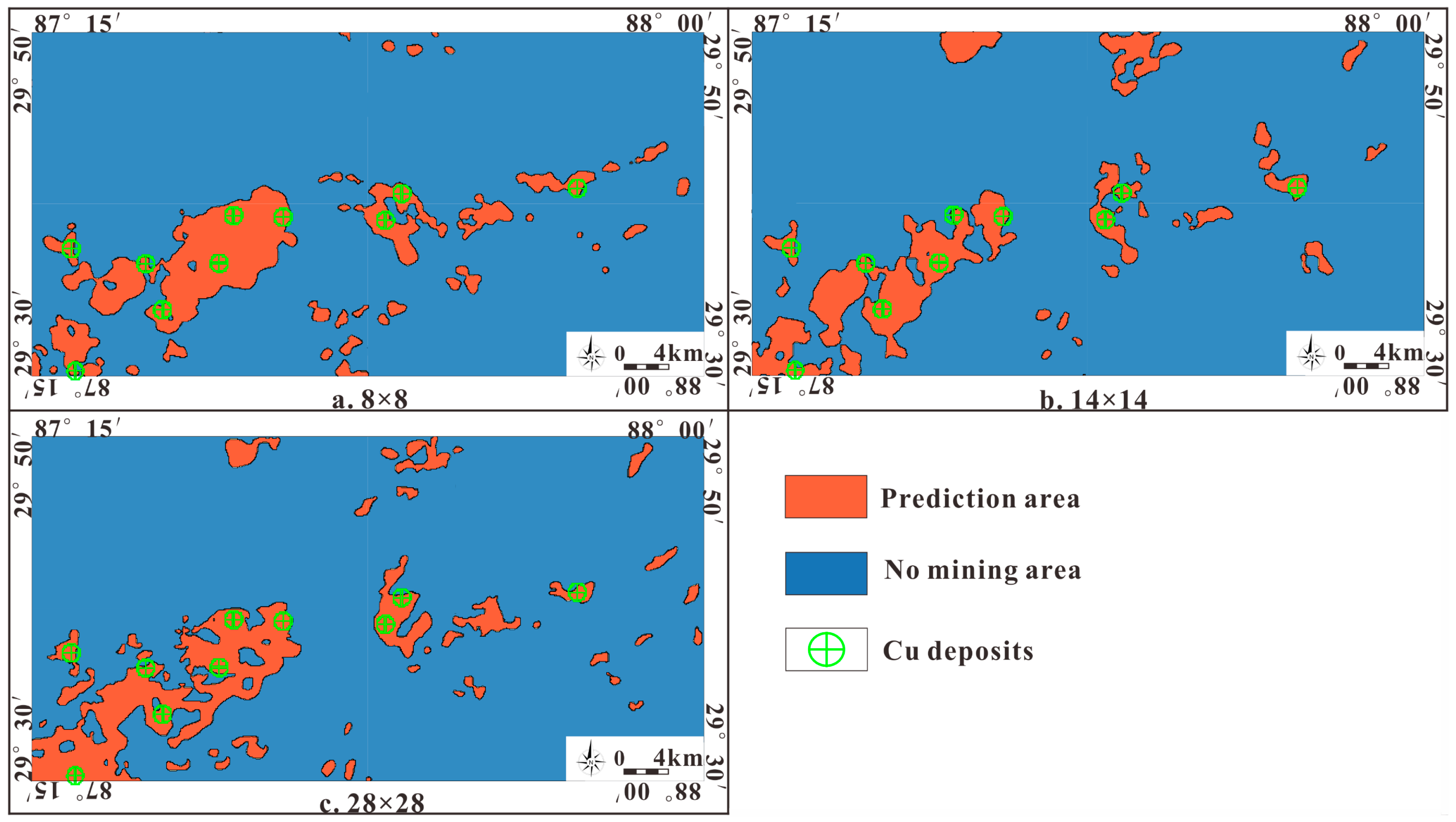
4.2.1. Influence of Window Size on the Prediction Results

The window parameters of a convolutional neural network can greatly affect the computational accuracy. During calculation, the calculation data in the window will be allocated to the center point of the window, so the selection of the window size is particularly important. The prediction results when the windows are 8 × 8, 14 × 14, and 28 × 28 of Cu deposits are shown in Figure 10. The results show that the window of 14 × 14 can make the prediction area more accurate, and the accuracy rate can reach 91.7%.

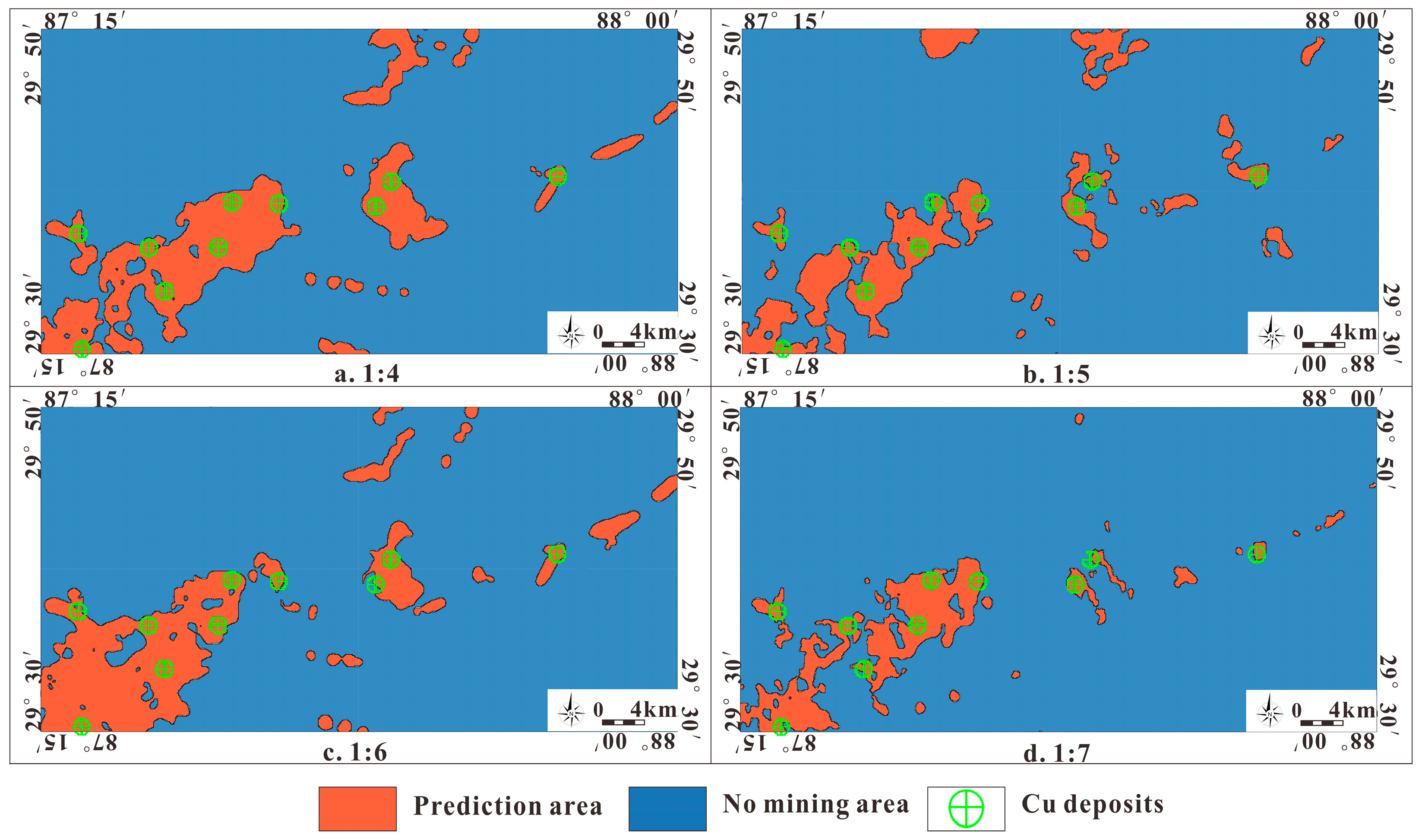
4.2.2. Influence of the Ratio of the Number of Positive and Negative Samples on the Prediction Results

The negative sample data are constructed by randomly sampling the nonmineral area. Here, the influence of different ratios of the number of ore-bearing samples to the number of non-ore samples on the prediction results is examined, as shown in Figure 11.

The results show that there were significant differences in the extent of the predicted regions for the four ratios. However, when the ratio is 1:5, all known deposits can be successfully predicted, and the prediction area is more accurate, with an accuracy rate of 91.7%.

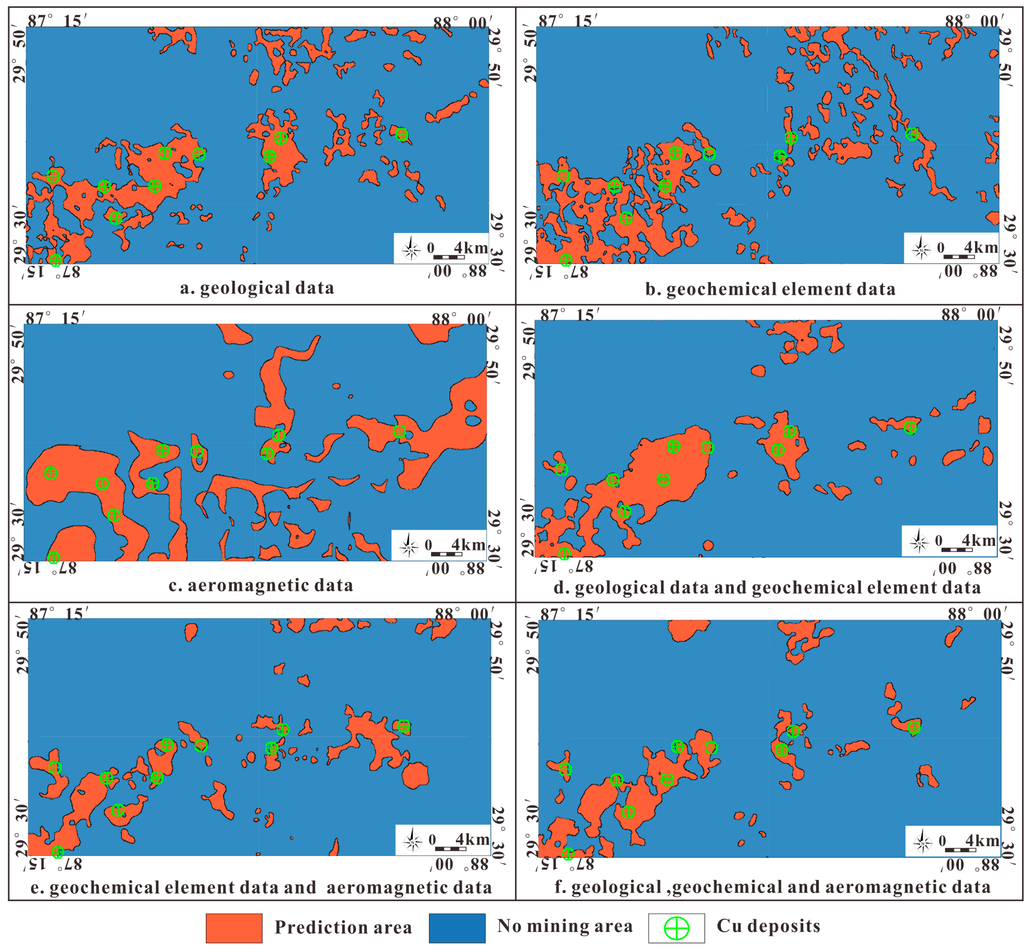
4.2.3. Influence of Different Datasets on the Prediction Results

This paper tests the influence of different input data on prediction, as shown in Figure 12. The results show that when a single type of data is input to make predictions, the prediction results have great instability (Figure 12a,b,c). When combining different kinds of data as input datasets, the results are relatively stable (Figure 12d,e,f). At the same time, it is found that the result of inputting all data into training is the best, and the predicted result area completely contains the known deposits, and the accuracy rate can reach 91.7%.

4.2.4. Prediction Results

There are 12 kinds of data in this experimental data set, including 2 kinds of geological data, 6 kinds of geochemical exploration data, and 4 kinds of aeromagnetic data.

The difference in prediction parameters will greatly affect the data processing ability of the model. Therefore, it is necessary to adjust and set various parameters according to the type, characteristics, and shape of the data, among which parameters such as the window size and the ratio of positive and negative samples determine the recognition ability of the model. This paper uses all the data and sets a window size of 14 × 14 grid cells (the actual range covered is equivalent to 700 m × 700 m) and a positive and negative sample ratio of 1:5 for prospecting prediction of Cu deposits. The model was trained and verified for 200 rounds, and its training accuracy and loss changes are shown in Figure 13.

The model was trained and validated for 200 rounds using the above parameters and datasets. According to the data, the model accuracy reaches 97.8% after multiple iterations of training, indicating that the model has high accuracy. Additionally, as the iteration loss gradually decreases, the loss gradually stabilizes at 0.08 in the 50th iteration, indicating that the actual output is similar to the expected output, and the model converges on the best effect. These results indicate that the final model should be considered valid.

The spatial distribution of Cu in the prospecting prospects identified by the final model is shown in Figure 14. The prediction results indicate that on the basis of the previous prediction results, the model obtained six favorable prospecting areas (purple boxes) in the study area. They are mainly oriented in the NE direction, and the prediction results are basically consistent with the locations of the high-value areas of the geological boundary influence intensity and fault influence intensity. The prediction area accounts for 9.5% of the total area, and all known Cu deposits and mineral occurrences plot in the prediction area.

The geological conditions of each prediction area are as follows.

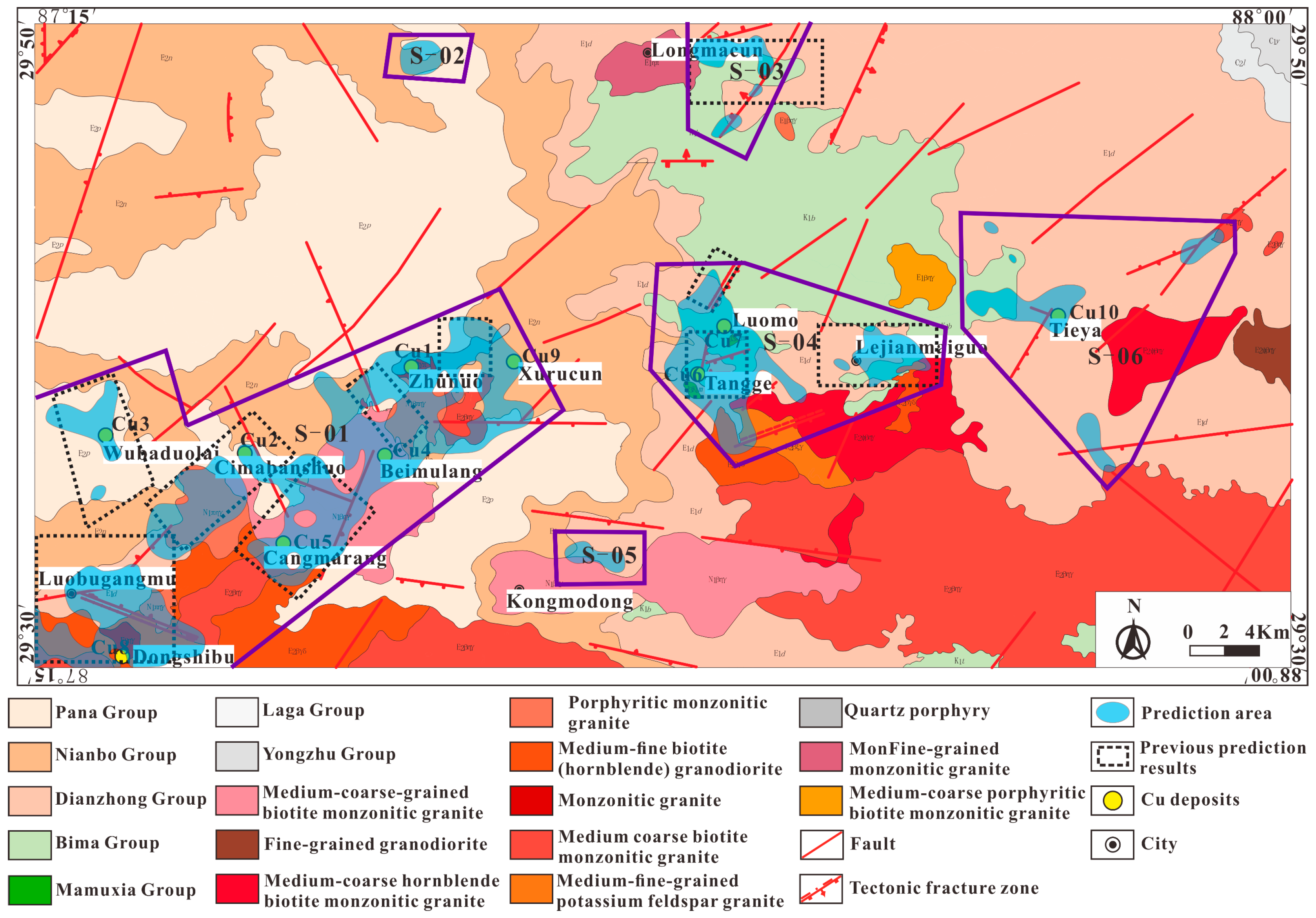
• The S-01 prediction areas are located in the southwestern corner of the study area, and the prediction area is small. Cu1, Cu2, Cu3, Cu4, Cu5, Cu8, and Cu9 all plot within the prediction area. The main outcrops are the Paleogene Nianbo Group, the Pana Group, and the Dianzhong Group, a large portion of the prediction area was intruded by Eocene granites and Miocene granites, many NE- and NW-trending fault structures are present, porphyry-type Cu mineralization is widespread, Cu anomalies and Cu–Mo anomalies are obvious in the area, and the prediction area has good prospecting prospects for Cu deposits.
• S-02 is located in the northwestern part of the study area and is part of the northern strong magnetic anomaly area, and the predicted area is small. The Nianbo Group and the Pana Group are mainly exposed, and NW-trending faults are developed in the area.
• S-03 is located in the northern part of the study area and is part of the northern strong magnetic anomaly area. The Lower Cretaceous Bima Group and Paleogene Dianzhong Group are mainly exposed. They were intruded by Paleocene granite; several NE-trending faults were mainly developed, which was favorable for ore blending and accommodating mineral precipitation and enrichment; and it was dominated by obvious Pb–Zn anomalies and no Cu anomalies.
• S-04 is located in the middle of the study area and belongs to the central negative magnetic anomaly area. The Lower Cretaceous Bima Group and Paleogene Dianzhong Group are mainly exposed. The predicted area is intruded by Eocene granite, the area contains Cu6 and Cu7, and NE-trending faults are well developed. The geochemical anomalies are dominated by Au–Mo, the Dianzhong Group volcanic rocks are thickly covered, and the Miocene plutons are not exposed. It is very likely that the metallization is deep, the denudation is less, and the deep Cu ore body is buried deeply, resulting in no Cu anomaly on the surface. It is speculated that the area has good prospecting prospects for Cu deposits.
• S-05 is located in the south-central part of the study area. The Paleogene Nianbo Group and Dianzhong Group are mainly exposed at the surface. The strata were intruded by Miocene granites in a large area; the strata developed near E–W-trending faults, showing a certain possibility of mineralization.
• S-06 is located in the eastern part of the study area, and the Lower Cretaceous Bima Group and Paleogene Dianzhong Group are mainly exposed. These strata are mainly intruded by Eocene granites. The faults are well developed, and they are mainly NE-trending, NW-trending, and nearly E–W-trending; no obvious geochemical anomalies were found.

5. Discussion

To test the superiority of the CNN2D-SENet model, the weight of evidence (WOE) method and the CNN2D were also used for prediction, and the prediction results of the CNN2D-SENet model, the WOE, and the CNN2D were compared (Figure 15).

The weight of evidence method is a geostatistical method proposed by the Canadian mathematical geologist Agterberg; this method predicts mineral prospecting areas through the superposition and composite analysis of some geological information related to mineralization [43,44]. Each type of geological information is an evidence factor for prospecting prediction, and the contribution of each evidence factor to prospecting prediction is determined by the weight of this factor. Then, the probability value of mineral development at any position in space is calculated to delineate the predicted target areas at different levels [45,46,47].

Since the weight-of-evidence method needs to rely on the experience and knowledge of the prospectors in the process of prospecting, the prediction results of the deep neural network that can learn independently are more objective and reliable.

This paper determines which model is more advantageous by examining the model’s ability to predict “known deposits” from known deposits. As shown in Figure 15, Cu1, Cu2, and Cu8 (green circles in Figure 15) are eliminated here, and predictions are made through the remaining seven known deposits and mineral occurrences. The comparison results show that the prediction results of the three methods have a certain similarity, and they are all consistent with the previous prediction results and predict new favorable areas for prospecting. However, there are still large differences in the predicted regions. Significant differences are as follows.

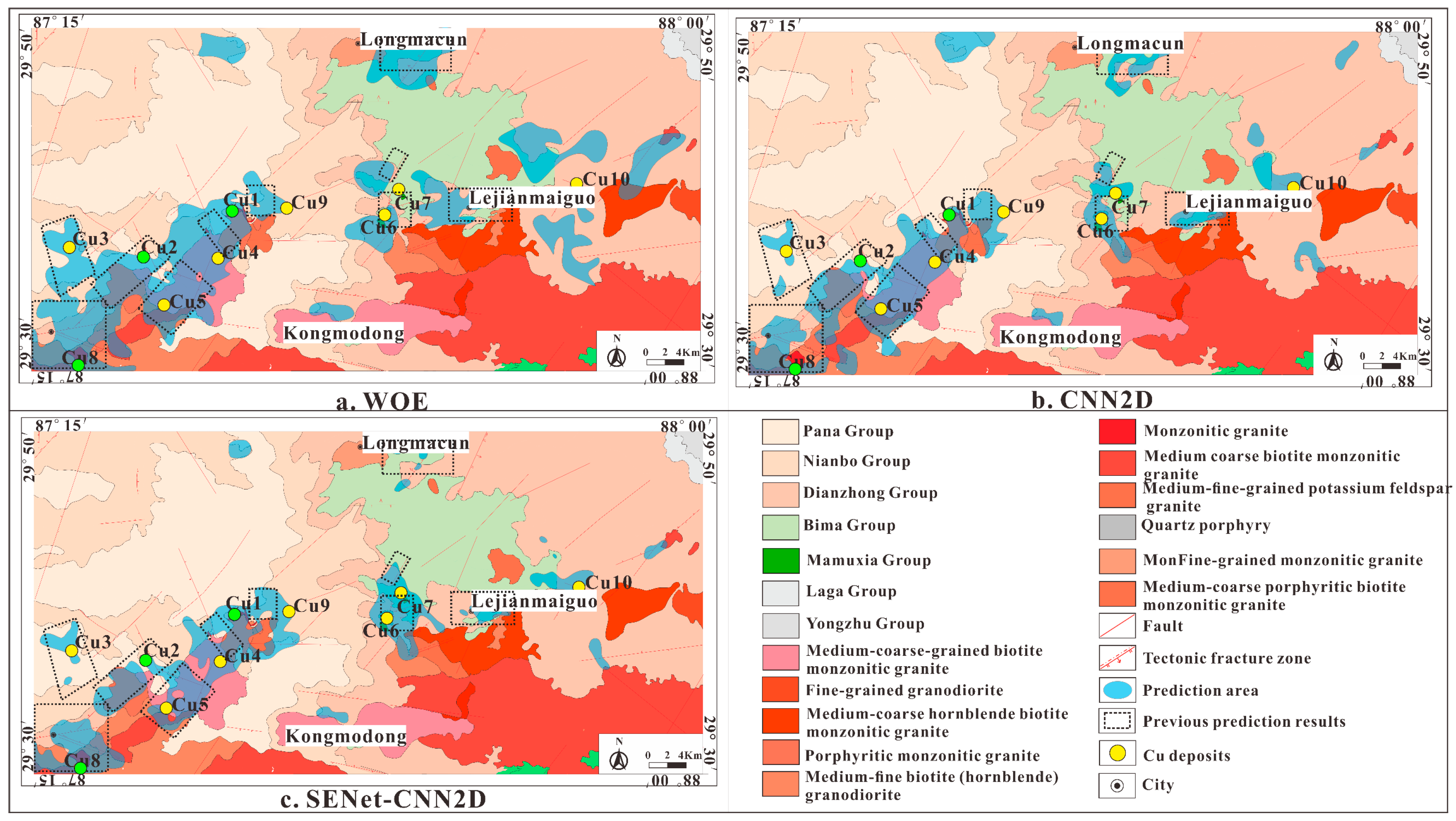
• The prediction area based on the WOE method is relatively large, accounting for 15.3% of the total area; the two methods based on deep learning have a smaller prediction area, such that the prediction area of CNN2D accounts for 9.2%, while the CNN2D-SENet model accounts for only 8.3%.
• The prediction method based on the CNN2D-SENet model successfully predicted three known deposits that were eliminated. However, Cu2 did not successfully fall within the prediction area of the CNN2D model. In addition, although Cu1, Cu2, and Cu8 were successfully predicted using the WOE method, Cu6, Cu7, and Cu10 did not fall within the prediction area. Considering that there is only one “evidence” layer (NE-trending fault) near Cu6 and Cu7, the metallogenic probability is low, and no good metallogenic possibility is shown. There are two “evidence” layers (Dianzhong Group and NE-trending fault) near Cu10, but Cu10 is far from the fault. The WOE method selects features by calculating weights, so breaks that exceed a certain distance have negative weights.
• By comparing the prediction results of the predecessors, it was found that the prediction results of the CNN2D-SENet model and the WOE method have a good fit and consistency with the prediction results of the predecessors. The prediction results of the CNN2D model also have a certain consistency with the prediction results of the predecessors, but the fit is general.

In summary, among the three supervised learning methods, the CNN2D-SENet model can be relatively successfully applied to prospecting prediction.

6. Conclusions

• The SENet network can selectively enhance beneficial feature channels while suppressing useless feature channels according to global information and finally achieve adaptive calibration of feature channels. The introduction of SENet to CNN2D helps to achieve a network model with better performance and improve the prediction accuracy.
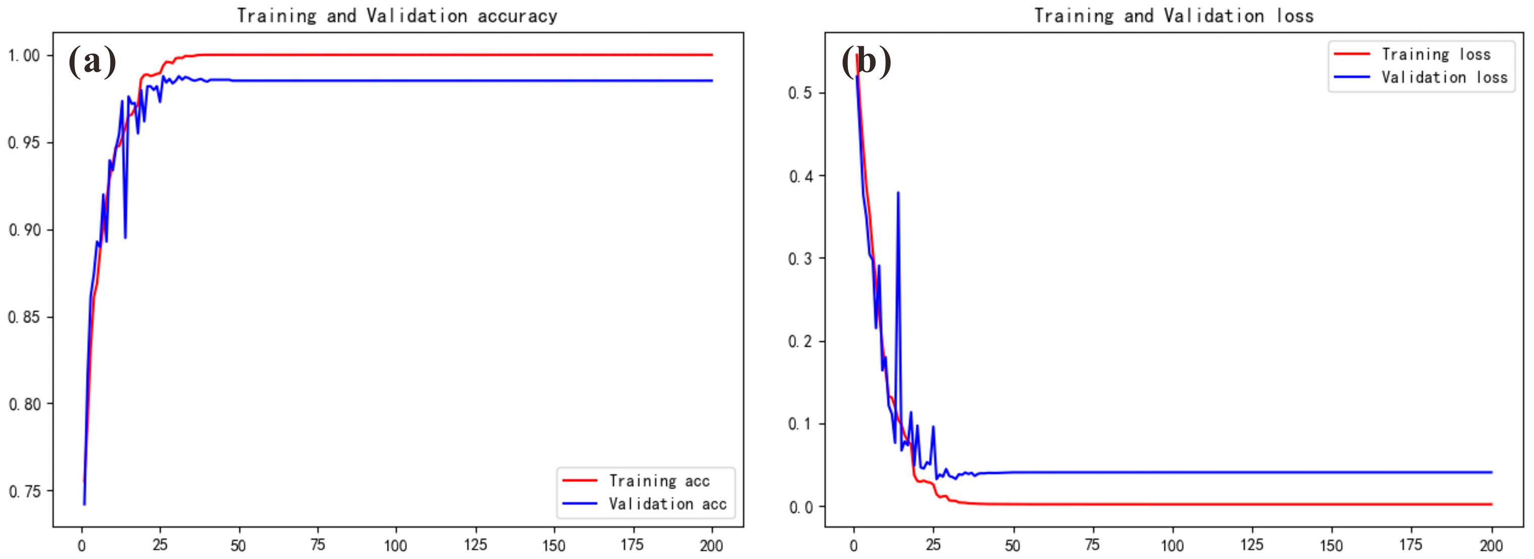
• To determine the optimal value of the model hyperparameters, a series of preset values were set for each parameter, and a large number of experiments were carried out. The results showed that all the data were selected, the window size was set to 14 × 14, and the ratio of positive to negative samples was set to 1:5 to obtain the optimal prediction result.
• The prospecting and prediction method based on the CNN2D-SENet model successfully delineated six Cu deposit prospecting areas in the Zhunuo mineral concentration area, which is consistent with the previous prediction results. Compared with the traditional WOE method and the typical CNN2D, better prediction results were obtained.

References

1. Barik, R.K.; Misra, C.; Lenka, R.K.; Dubey, H.; Mankodiya, K. Hybrid mist-cloud systems for large scale geospatial big data analytics and processing: Opportunities and challenges. Arab. J. Geosci. 2019, 12, 32. [Google Scholar] [CrossRef]
2. Cai, H.H.; Xu, Y.Y.; Li, Z.X.; Cao, H.H.; Feng, Y.X.; Chen, S.Q.; Li, Y.S. The division of metallogenic prospective areas based on convolutional neural network model: A case study of the Daqiao gold polymetallic deposit. Geol. Bull. China 2019, 38, 1999–2009, (In Chinese with English abstract). [Google Scholar]
3. Chen, L.; Guan, Q.; Xiong, Y.; Liang, J.; Wang, Y.; Xu, Y. A Spatially Constrained Multi-Autoencoder approach for multivariate geochemical anomaly recognition. Comput. Geosci. 2019, 125, 43–54. [Google Scholar] [CrossRef]
4. Ran, X.; Xue, L.; Zhang, Y.; Liu, Z.; Sang, X.; He, J. Rock Classification from Field Image Patches Analyzed Using a Deep Convolutional Neural Network. Mathematics 2019, 7, 755. [Google Scholar] [CrossRef]
5. Zuo, R.; Xiong, Y. Big Data Analytics of Identifying Geochemical Anomalies Supported by Machine Learning Methods. Nat. Resour. Res. 2017, 27, 5–13. [Google Scholar] [CrossRef]
6. Holden, E.-J.; Liu, W.; Horrocks, T.; Wang, R.; Wedge, D.; Duuring, P.; Beardsmore, T. GeoDocA—Fast analysis of geological content in mineral exploration reports: A text mining approach. Ore Geol. Rev. 2019, 111, 102919. [Google Scholar] [CrossRef]
7. Xiong, Y.; Zuo, R. Recognizing multivariate geochemical anomalies for mineral exploration by combining deep learning and one-class support vector machine. Comput. Geosci. 2020, 140, 104484. [Google Scholar] [CrossRef]
8. Xiong, Y.; Zuo, R. A positive and unlabeled learning algorithm for mineral prospectivity mapping. Comput. Geosci. 2021, 147, 104667. [Google Scholar] [CrossRef]
9. Zhou, Y.Z.; Chen, S.; Zhang, Q.; Xiao, F.; Wang, S.G.; Liu, Y.P.; Jiao, S.T. Progress in Big Data and Mathematical Geosciences—Preface to Topics on Big Data and Mathematical Geoscience. Acta Petrol. Sin. 2018, 34, 255–263, (In Chinese with English abstract). [Google Scholar]
10. Li, T.; Zuo, R.; Xiong, Y.; Peng, Y. Random-Drop Data Augmentation of Deep Convolutional Neural Network for Mineral Prospectivity Mapping. Nat. Resour. Res. 2020, 30, 27–38. [Google Scholar] [CrossRef]
11. Zhang, S.; Carranza, E.J.M.; Wei, H.; Xiao, K.; Yang, F.; Xiang, J.; Zhang, S.; Xu, Y. Data-driven Mineral Prospectivity Mapping by Joint Application of Unsupervised Convolutional Auto-encoder Network and Supervised Convolutional Neural Network. Nat. Resour. Res. 2021, 30, 1011–1031. [Google Scholar] [CrossRef]
12. Zuo, R.G. Deep learning-based mining and integration of deep-level mineralization information. Bull. Mineral. Petrol. Geochem. 2019, 38, 53–60, (In Chinese with English abstract). [Google Scholar] [CrossRef]
13. Abedi, M.; Norouzi, G.H.; Torabi, S.A. Clustering of mineral prospectivity area as an unsupervised classification approach to explore copper deposit. Arab. J. Geosci. 2012, 6, 3601–3613. [Google Scholar] [CrossRef]
14. Paasche, H.; Eberle, D.G. Rapid integration of large airborne geophysical data suites using a fuzzy partitioning cluster algorithm: A tool for geological mapping and mineral exploration targeting. Explor. Geophys. 2009, 40, 277–287. [Google Scholar] [CrossRef]
15. Xu, S.T.; Zhou, Y.Z. Experimental study on intelligent identification of ore minerals under the microscope based on deep learning. Chin. J. Petrol. 2018, 34, 3244–3252, (In Chinese with English abstract). [Google Scholar]
16. Sang, X.; Xue, L.; Ran, X.; Li, X.; Liu, J.; Liu, Z. Intelligent High-Resolution Geological Mapping Based on SLIC-CNN. ISPRS Int. J. Geo-Informat. 2020, 9, 99. [Google Scholar] [CrossRef]
17. Liu, Y.P.; Zhu, L.X.; Zhou, Y.Z. Application of Convolutional Neural Network in Prospecting Prediction of Ore Deposits: Taking the Zhaojikou Pb-Zn Ore Deposit in Anhui Province as a Case. Acta Petrol. Sin. 2018, 34, 3217–3224, (In Chinese with English abstract). [Google Scholar]
18. Li, S.; Chen, J.P.; Xiang, J. Prospecting Information Extraction by Text Mining Based on Convolutional Neural Networks—A Case Study of the Lala Copper Deposit, China. IEEE Access 2018, 6, 52286–52297. [Google Scholar] [CrossRef]
19. Li, H.; Li, X.; Yuan, F.; Jowitt, S.M.; Zhang, M.; Zhou, J.; Zhou, T.; Li, X.; Ge, C.; Wu, B. Convolutional neural network and transfer learning based mineral prospectivity modeling for geochemical exploration of Au mineralization within the Guandian–Zhangbaling area, Anhui Province, China. Appl. Geochem. 2020, 122, 104747. [Google Scholar] [CrossRef]
20. He, K.; Zhang, X.; Ren, S.; Sun, J. Deep residual learning for image recognition. In Proceedings of the IEEE Computer Society Conference on Computer Vision and Pattern Recognition (CVPR), Las Vegas, NV, USA, 27–30 June 2016; pp. 770–778. [Google Scholar] [CrossRef]
21. Simonyan, K.; Zisserman, A. Very Deep Convolutional Networks for Large-Scale Image Recognition. arXiv 2015, arXiv:1409.1556. [Google Scholar] [CrossRef]
22. Szegedy, C.; Liu, W.; Jia, Y.; Sermanet, P.; Reed, S.; Anguelov, D.; Erhan, D.; Vanhoucke, V.; Rabinovich, A.; Liu, W.; et al. Going deeper with convolutions. In Proceedings of the 2015 IEEE Conference on Computer Vision and Pattern Recognition (CVPR), Boston, MA, USA, 7–12 June 2015; pp. 1–9. [Google Scholar] [CrossRef]
23. Vaswani, A.; Shazeer, N.; Parmar, N.; Uszkoreit, J.; Jones, L.; Gomez, A.N.; Kaiser, L.; Polosukhin, I. In Attention Is All You Need. arXiv 2017, arXiv:1706.03762. [Google Scholar] [CrossRef]
24. Hu, J.; Shen, L.; Albanie, S.; Sun, G.; Wu, E. Squeeze-and-Excitation Networks. IEEE Trans. Pattern Anal. Mach. Intell. 2020, 42, 2011–2023. [Google Scholar] [CrossRef]
25. Liu, H.; Peng, C.; Xue, L.; Li, W.; Xu, C.; Jofrisse, C.S. Non-seismic geophysical analysis of potential geothermal resources in the Longgang Block, Northeast China. Earth Planet. Phys. 2022, 6, 576–591. [Google Scholar] [CrossRef]
26. Yin, A.; Harrison, T.M. Geologic evolution of the Himalayan-Tibetan orogen. Annu. Rev. Earth Planet. Sci. 2000, 28, 211–280. [Google Scholar] [CrossRef]
27. Hou, Z.Q.; Zheng, Y.C.; Yang, Z.M.; Yang, Z.S. Continental Collision Metallogenesis: I. Gangdise Cenozoic Porphyry Metallogenic System. Depos. Geol. 2012, 31, 647–670, (In Chinese with English abstract). [Google Scholar] [CrossRef]
28. Ji, W.-Q.; Wu, F.-Y.; Chung, S.-L.; Li, J.-X.; Liu, C.-Z. Zircon U–Pb geochronology and Hf isotopic constraints on petrogenesis of the Gangdese batholith, southern Tibet. Chem. Geol. 2009, 262, 229–245. [Google Scholar] [CrossRef]
29. Lee, H.-Y.; Chung, S.-L.; Ji, J.; Qian, Q.; Gallet, S.; Lo, C.-H.; Lee, T.-Y.; Zhang, Q. Geochemical and Sr–Nd isotopic constraints on the genesis of the Cenozoic Linzizong volcanic successions, southern Tibet. J. Asian Earth Sci. 2012, 53, 96–114. [Google Scholar] [CrossRef]
30. Ge, L.S.; Deng, J.; Yang, L.Q.; Zou, Y.L.; Xing, J.B.; Yuan, S.S.; Wu, Y.H. Meso-Cenozoic mid-acid intrusive magmatism and tectonic evolution in the Gangdise block, Tibet. Geol. Resour. 2016, 15, 1–10, (In Chinese with English abstract). [Google Scholar]
31. Hou, Z.Q.; Mo, X.X.; Gao, Y.F.; Qu, X.M.; Meng, X.J. Adakite: A possible important ore-bearing parent rock for porphyry copper deposits—Taking Tibet and Chile porphyry copper deposits for example. Depos. Geol. 2003, 22, 1–12, (In Chinese with English abstract). [Google Scholar]
32. Zheng, Y.Y.; Gao, S.B.; Zhang, D.Q.; Fan, Z.H.; Zhang, G.Y.; Ma, G.T. The great significance and enlightenment of the discovery of the Juno porphyry copper deposit in Tibet. Earth Sci. Front. 2006, 13, 233–239, (In Chinese with English abstract). [Google Scholar]
33. Zheng, Y.Y.; Duo, J.; Zhang, G.Y.; Gao, S.B.; Fan, Z.H. The discovery process and significance of the Jiru porphyry copper deposit in Tibet. Depos. Geol. 2007, 26, 317–321, (In Chinese with English abstract). [Google Scholar]
34. Zheng, Y.Y.; Zhang, G.Y.; Xu, R.K.; Gao, S.B.; Pang, Y.C.; Cao, L. Age constraints of diagenesis and mineralization of the Juno porphyry copper deposit in Gangdise, Tibet. Sci. Bull. 2007, 52, 2542–2548, (In Chinese with English abstract). [Google Scholar] [CrossRef]
35. Huang, Y.; Ding, J.; Li, G.M.; Dai, J.; Yan, G.Q.; Wang, G.; Liu, X.F. U-Pb age, Hf isotopic composition and mineralization significance of intrusive zircon in copper-molybdenum-gold mining area of Zhunuo porphyry in Tibet. Acta Geol. Sin. 2015, 89, 99–108, (In Chinese with English abstract). [Google Scholar]
36. Sun, X.; Lu, Y.; McCuaig, T.C.; Zheng, Y.-Y.; Chang, H.-F.; Guo, F.; Xu, L.-J. Miocene Ultrapotassic, High-Mg Dioritic, and Adakite-like Rocks from Zhunuo in Southern Tibet: Implications for Mantle Metasomatism and Porphyry Copper Mineralization in Collisional Orogens. J. Petrol. 2018, 59, 341–386. [Google Scholar] [CrossRef]
37. Peng, C.; Xue, L.-F.; Zhu, M.; Chai, Y.; Liu, W.-Y. The location and evolution of the tectonic boundary between the Paleoproterozoic Jiao-Liao-Ji Belt and the Longgang Block, northeast China. Precambr. Res. 2016, 272, 18–38. [Google Scholar] [CrossRef]
38. Wu, S.; Zheng, Y.; Sun, X. Subduction metasomatism and collision-related metamorphic dehydration controls on the fertility of porphyry copper ore-forming high Sr/Y magma in Tibet. Ore Geol. Rev. 2016, 73, 83–103. [Google Scholar] [CrossRef]
39. Li, Z.T.; Xue, L.F.; Ran, X.J.; Li, Y.S.; Dong, G.Q.; Li, Y.B.; Dai, J.H. Intelligent prospecting and prediction method based on convolutional neural network—Taking the copper mine in Longshoushan area of Gansu as an example. J. Jilin Univ. 2022, 52, 418–433, (In Chinese with English abstract). [Google Scholar] [CrossRef]
40. Wang, H.X.; Zhou, J.Q.; Gu, C.H.; Lin, H. Design of activation functions in convolutional neural networks for image classification. J. Zhejiang Univ. 2019, 53, 1363–1373, (In Chinese with English abstract). [Google Scholar] [CrossRef]
41. Liu, W.J.; Liang, X.J.; Qu, H.C. Study on the Learning Performance of Convolutional Neural Networks with Different Pooling Models. Chin. J. Image Graph. 2016, 21, 1178–1190, (In Chinese with English abstract). [Google Scholar]
42. Ding, K.; Xue, L.; Ran, X.; Wang, J.; Yan, Q. Siamese network based prospecting prediction method: A case study from the Au deposit in the Chongli mineral concentrate area in Zhangjiakou, Hebei Province, China. Ore Geol. Rev. 2022, 148, 105024. [Google Scholar] [CrossRef]
43. Li, Y.-S.; Peng, C.; Ran, X.-J.; Xue, L.-F.; Chai, S.-L. Soil geochemical prospecting prediction method based on deep convolutional neural networks-Taking Daqiao Gold Mine in Gansu Province, China as an example. China Geol. 2022, 5, 71–83. [Google Scholar] [CrossRef]
44. Xiong, Y.; Zuo, R. Recognition of geochemical anomalies using a deep autoencoder network. Comput. Geosci. 2016, 86, 75–82. [Google Scholar] [CrossRef]
45. Agterberg, F.P.; Bonham-Carter, G.F.; Wright, D.F. Statistical Pattern Integration for Mineral Exploration; Geological Survey of Canada Contribution No. 24088. In Computer Applications in Resource Estimation; Prediction and Assessment for Metals and Petroleum; Gaál, G., Merriam, D.F., Eds.; Pergamon Press: Amsterdam, The Netherlands, 1990; pp. 1–21. [Google Scholar] [CrossRef]
46. Agterberg, F.P.; Cheng, Q. Conditional Independence Test for Weights-of-Evidence Modeling. Nat. Resour. Res. 2002, 11, 249–255. [Google Scholar] [CrossRef]
47. Xiao, K.Y.; Zhang, X.H.; Chen, Z.H.; Song, G.Y.; Ge, Y.; Liu, D.L.; Wang, S.L.; Ning, S.N.; Cao, Y. Evidence weight method and information quantity method and their comparison in metallogenic prediction. Geophys. Geochem. Calc. Technol. 1999, 21, 223–226, (In Chinese with English abstract). [Google Scholar]
Figure 1. (a)—Tectonic zoning map of China (simplified and revised after [35]). (b) Distribution map of major volcanic–magmatic and porphyry deposits in the Lhasa Terrane, Tibet (simplified and revised from [36]). (c) Geological and mineral resources map of the Zhunuo integrated exploration area (modified from the mineral prospect survey report in Zhunuo, Tibet, and the special mapping and technology application and demonstration of the integrated exploration area in Zhunuo, Tibet). 1. Pana Group; 2. Nianbo Group; 3. Dianzhong Group; 4. Bima Group; 5. Mamuxia Group; 6. Laga Group; 7. Yongzhu Group; 8. Medium- to coarse-grained biotite monzonitic granite; 9. Fine-grained granodiorite; 10. Medium- to coarse-grained amphibole-bearing biotite monzogranite; 11. Porphyritic monzogranite; 12. Medium- to fine-grained biotite (amphibole) granodiorite; 13. Monzogranite; 14. Medium- to coarse-grained biotite monzogranite; 15. Medium- to fine-grained potassium feldspar granite; 16. Quartz porphyry; 17. Fine-grained monzonite; 18. Medium- to coarse-grained porphyry biotite monzonite; 19. Reverse fault; 20. Normal fault; 21. Structural fracture zone; 22. Unidentified fault; 23. Cu deposits (mineral occurrences); 24. City.
Minerals 13 00730 g001
Figure 2. CNN2D-SENet model architecture diagram.
Minerals 13 00730 g002
Figure 3. CNN2D model architecture diagram.
Minerals 13 00730 g003
Figure 4. Schematic diagram of the squeeze-excitation (SE) module.
Minerals 13 00730 g004
Figure 5. Flow chart of prospecting prediction based on the CNN2D-SENet model (edited by Ding et al. [40]).
Minerals 13 00730 g005
Figure 6. Schematic diagram of sample making of a sliding window (the window size is 3 × 3; ④⑤ mining areas are positive samples; ①②③ unknown areas are negative samples).
Minerals 13 00730 g006
Figure 7. Relationship between the influence intensity of the geological boundary (a) and the fault influence intensity (b) with the deposits and mineral occurrences.
Minerals 13 00730 g007
Figure 8. A 1:50,000 contour map of geochemical elements.
Minerals 13 00730 g008
Figure 9. A 1:50,000 aeromagnetic anomaly map and continuation map ((a)—aeromagnetic anomaly map; (b)—aeromagnetization pole map; (c)—upwards of 500 m; (d)—upwards of 1000 m).
Minerals 13 00730 g009
Figure 10. Comparison of the influence of window size on prediction results ((a) window size of 8 × 8; (b) window size of 14 × 14; (c) window size of 28 × 28).
Minerals 13 00730 g010
Figure 11. Comparison of the influence of positive and negative sample size ratios on prediction results ((a) ratio of 1:4; (b) ratio of 1:5; (c) ratio of 1:6; (d) ratio of 1:7).
Minerals 13 00730 g011
Figure 12. Comparison of the influence of different datasets on the prediction results ((a) geological data; (b) geochemical element data; (c) aeromagnetic data; (d) geological data and geochemical element data; (e) geochemical element data and aeromagnetic data; (f) geological data, geochemical element data, and aeromagnetic data).
Minerals 13 00730 g012
Figure 13. Accuracy and changes in the loss of the training model based on the CNN2D- SENet model (a) training and validation accuracy; (b) training and validation loss.
Minerals 13 00730 g013
Figure 14. Prediction results of Cu deposits (The blue semitransparent colored part of the figure is the obtained prediction area).
Minerals 13 00730 g014
Figure 15. Prediction results of the three methods (a) prediction results of Weight of Evidence Method; (b) prediction results of 2D Convolutional Neural Network; (c) prediction results of CNN2D-SENet).
Minerals 13 00730 g015