
Connecting Obsidian Artifacts with Their Sources Using Multivariate Statistical Analysis of LIBS Spectral Signatures
 , and
, and
Abstract
:
1. Introduction
2. Background
2.1. Obsidian
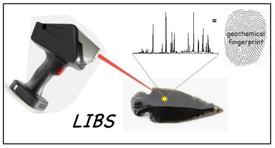
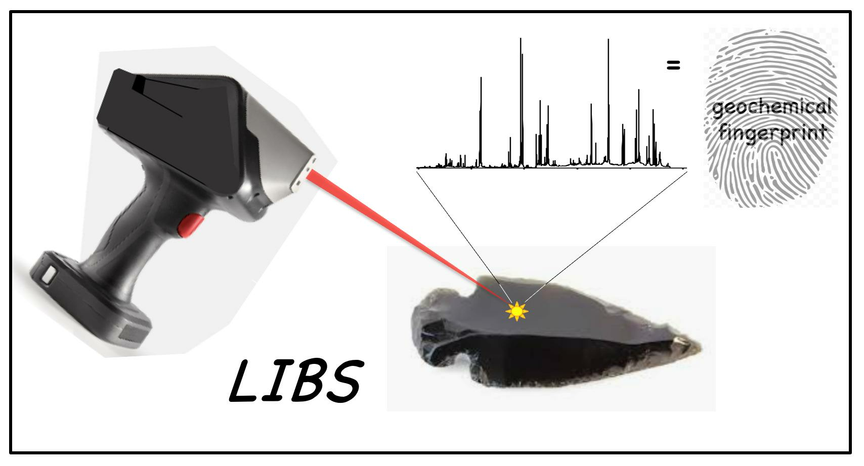
2.2. Geochemical Fingerprinting
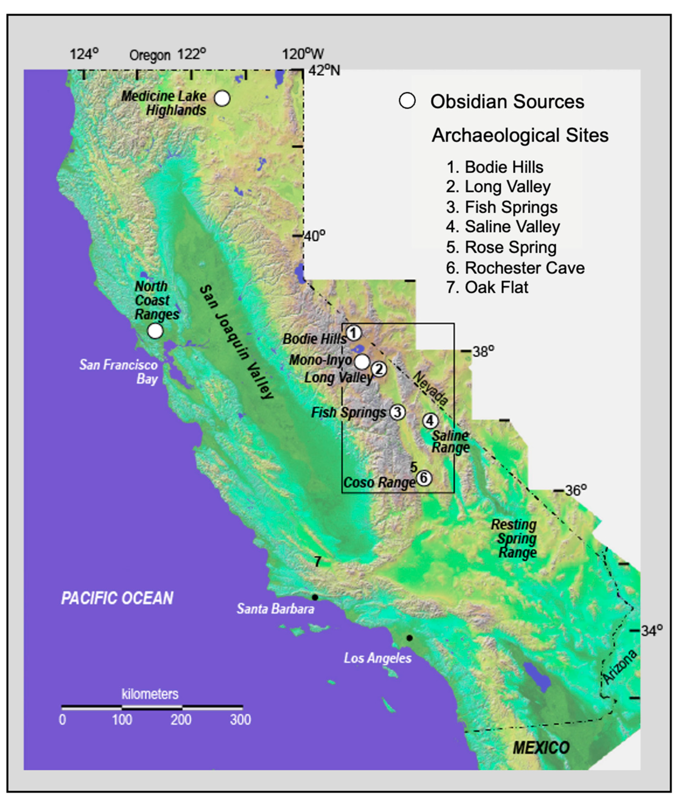
3. Obsidian Sources and Archeological Sites in North-Central California
3.1. Medicine Lake Highlands, Northern California
3.2. North Coast Ranges
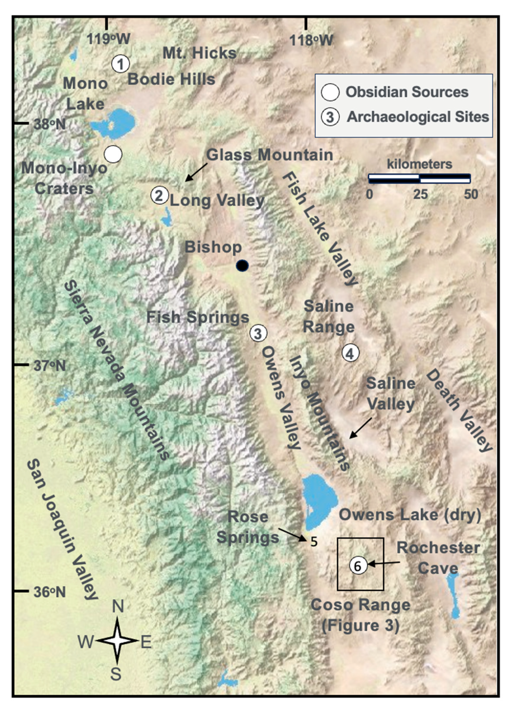
3.3. East-Central California
3.3.1. Bodie Hills
3.3.2. Long Valley Caldera and Mono-Inyo Craters
3.3.3. Saline Range and Inyo Mountains
3.3.4. Fish Springs
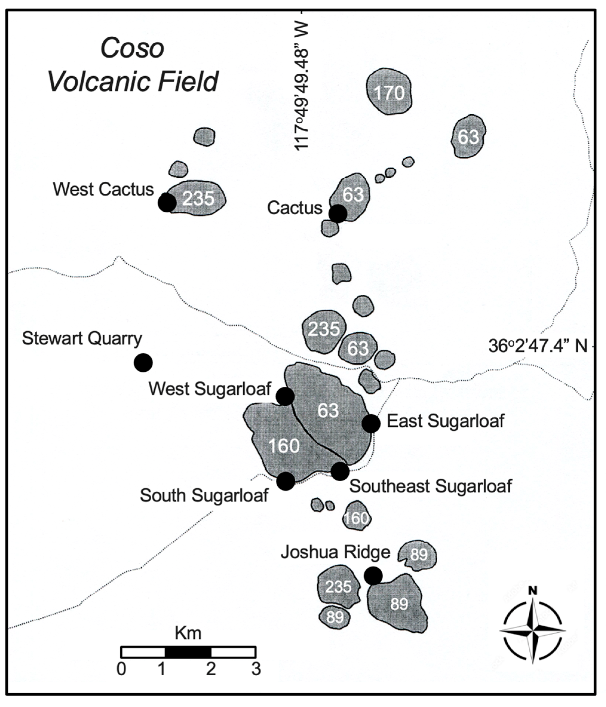
3.3.5. Coso Range
3.4. Oak Flat
4. Analytical Methodology
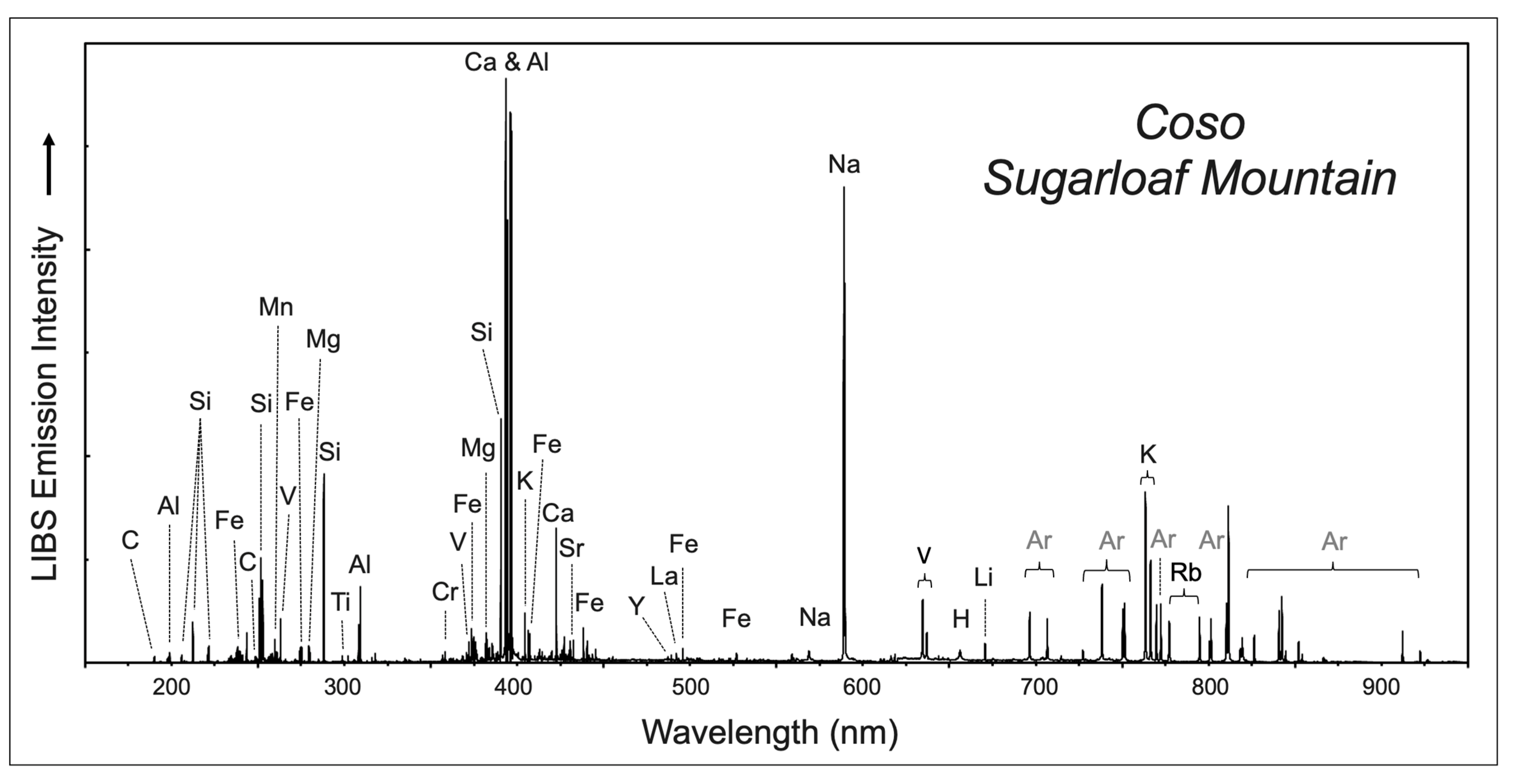
4.1. LIBS Analysis
4.2. Data Processing and Chemometric Analysis
4.2.1. Data Preprocessing
4.2.2. Spectral Similarity
4.2.3. Visualization
4.2.4. Sample Classification/Discrimination
5. Results
5.1. Obsidian Sources
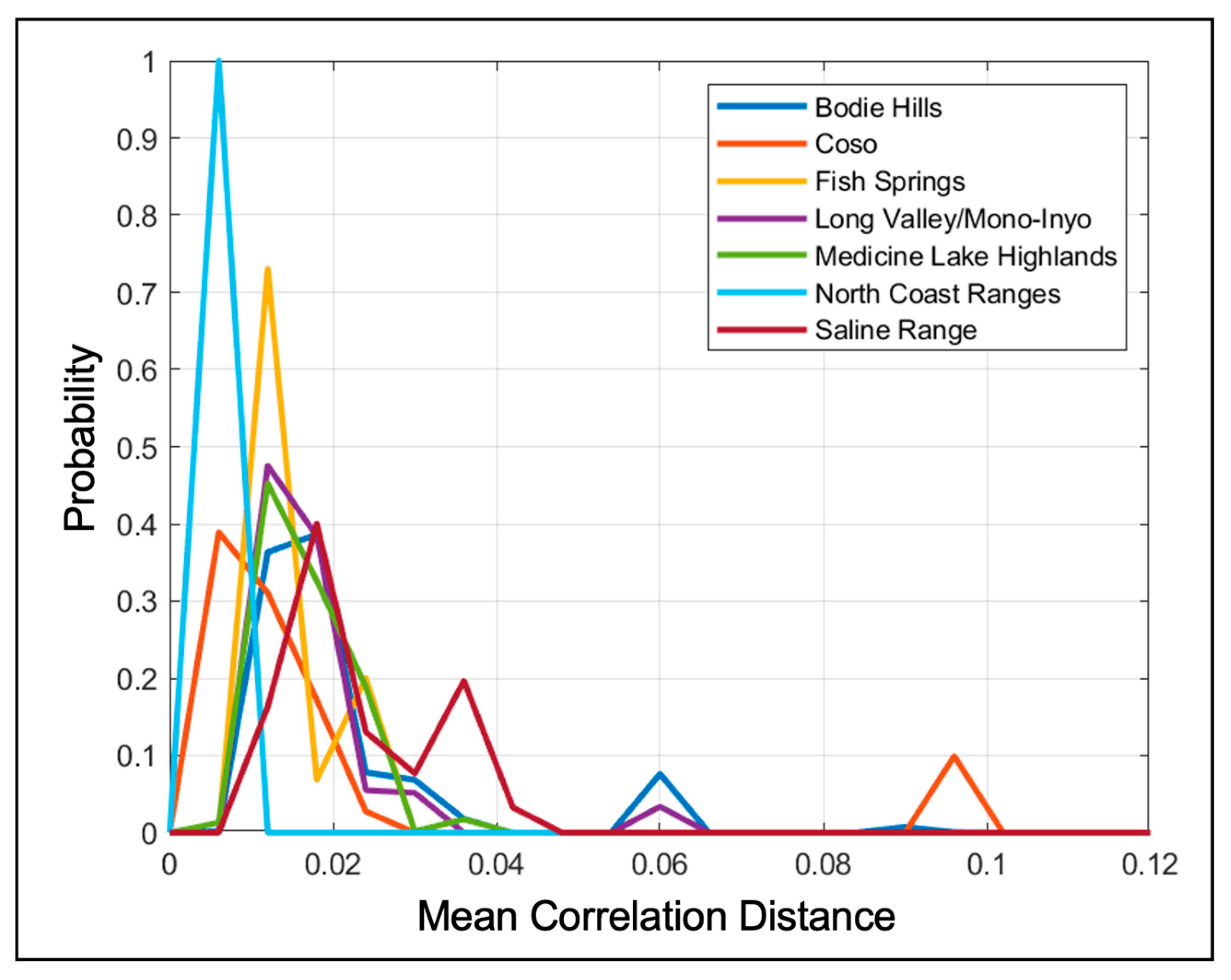
5.1.1. Source Similarity
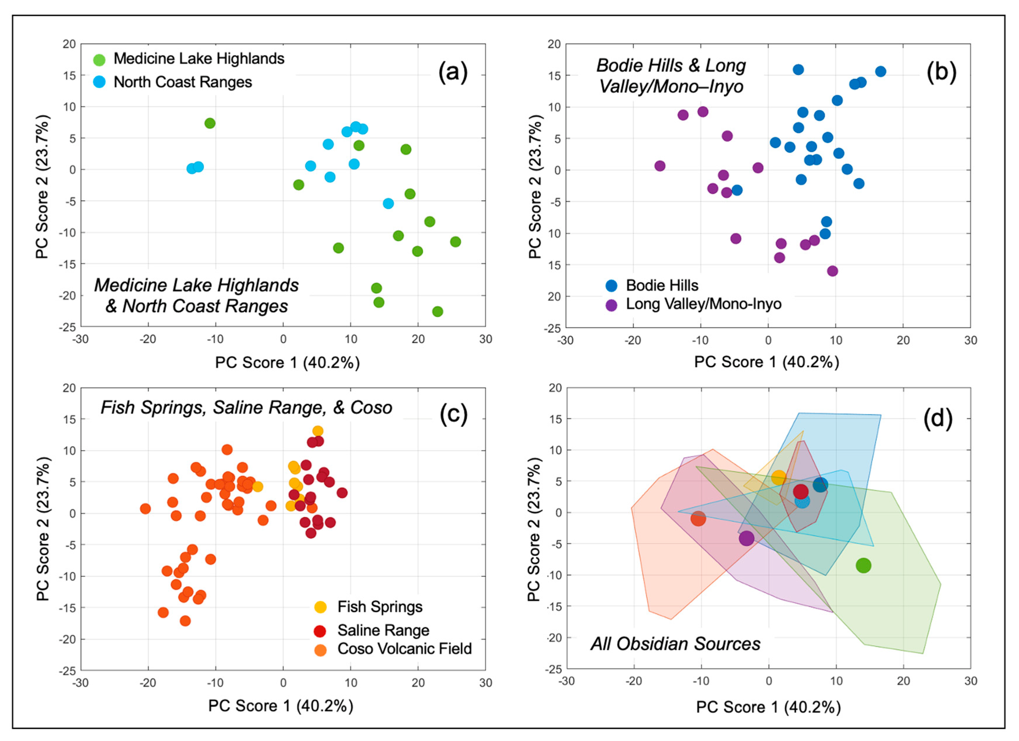
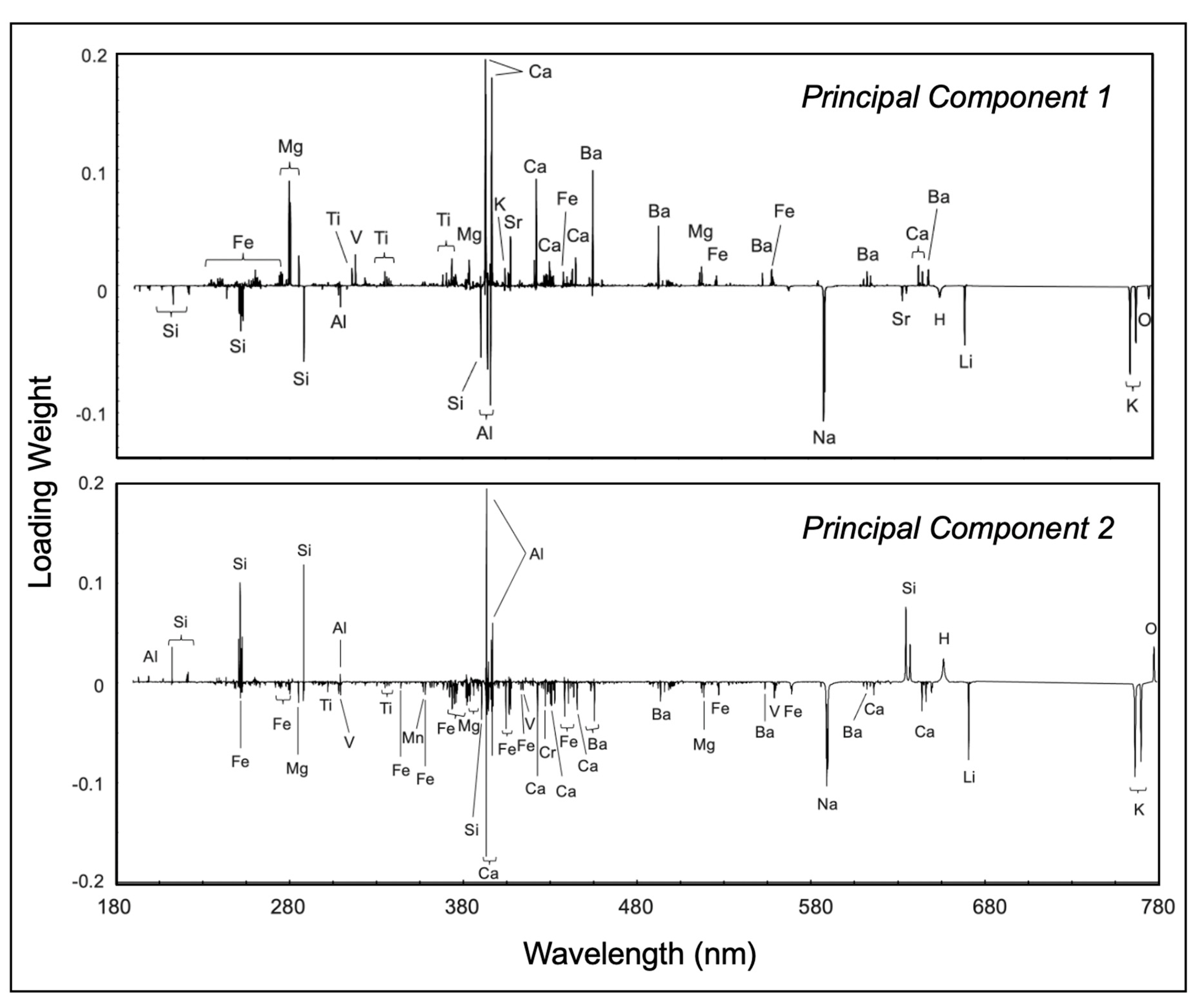
5.1.2. Source PCA
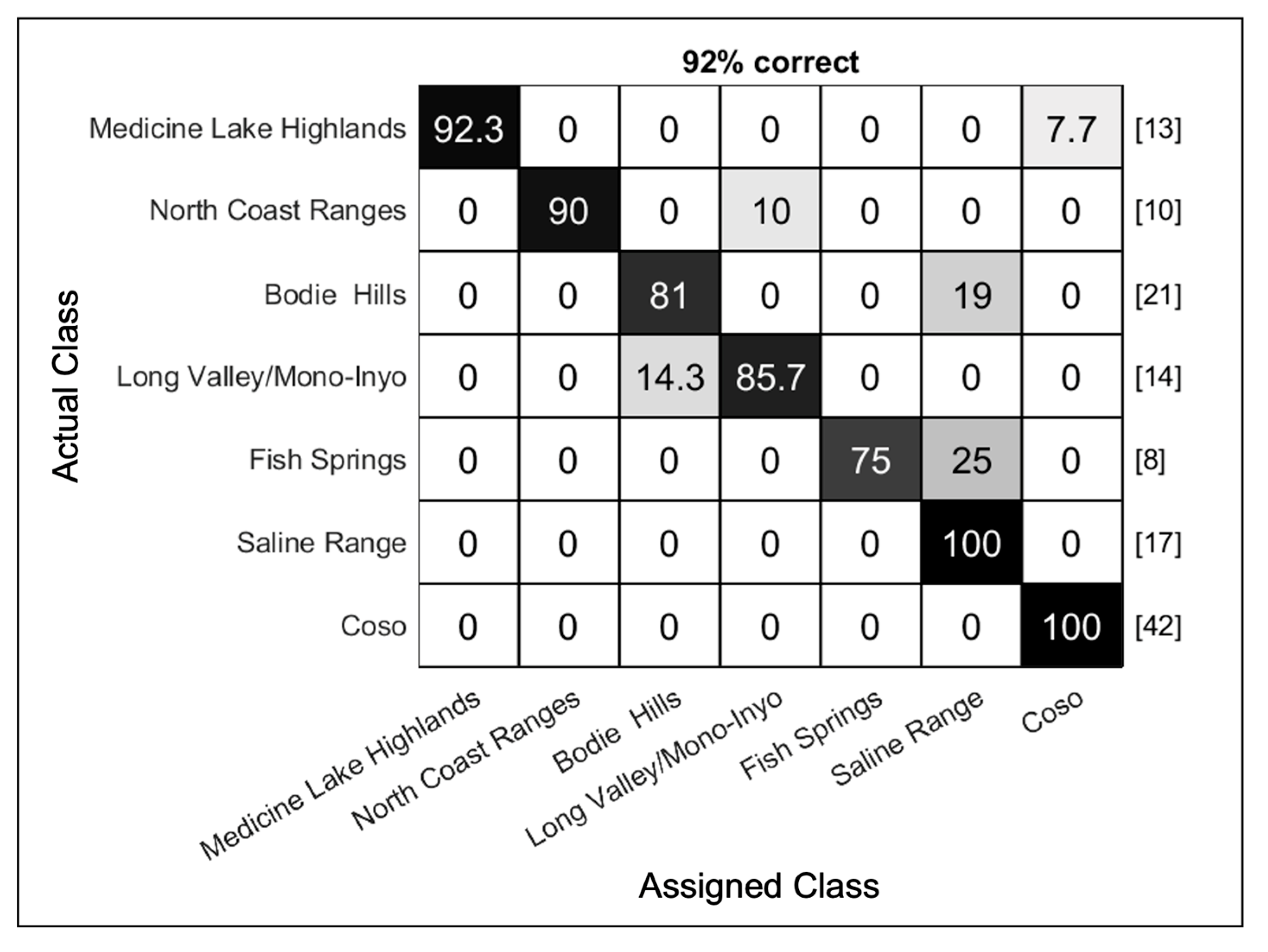
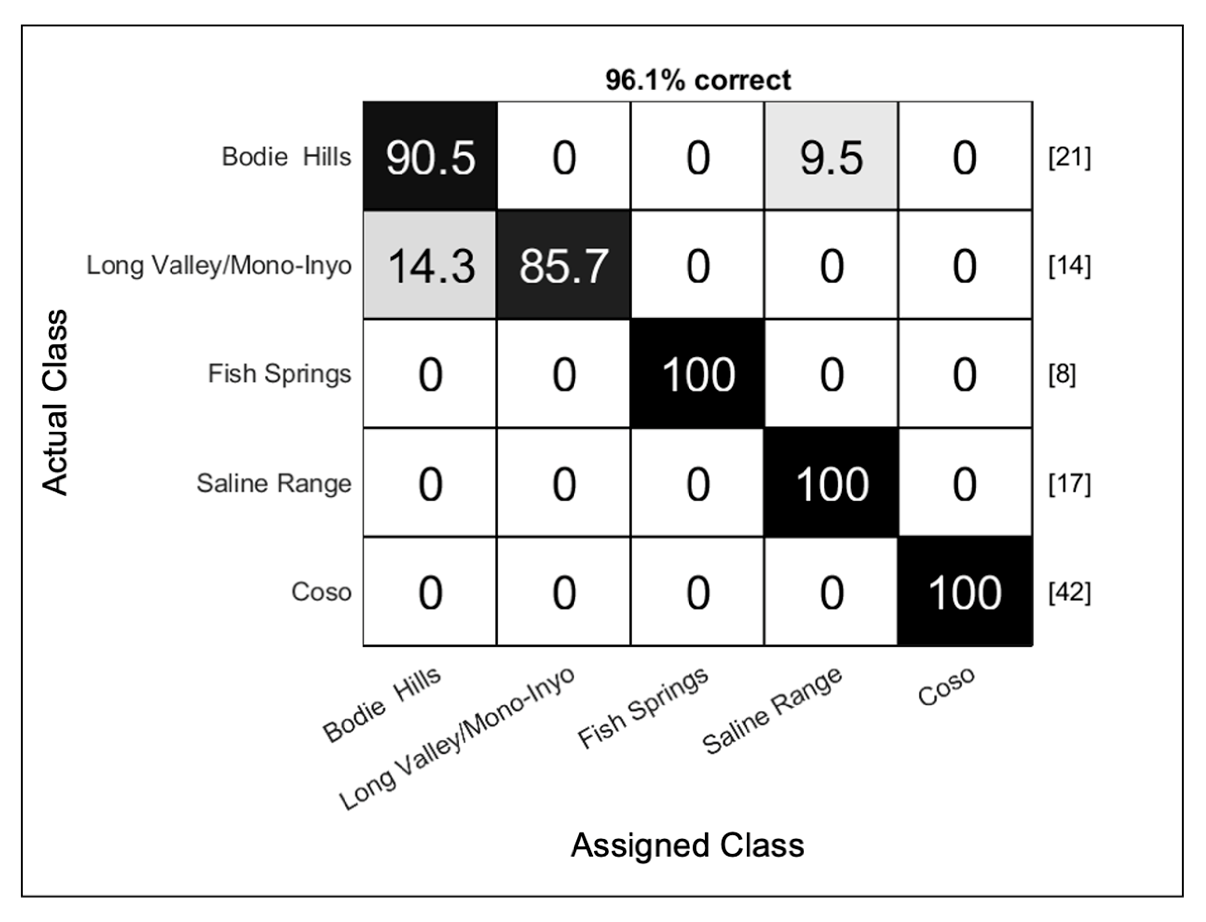
5.1.3. Source Discrimination
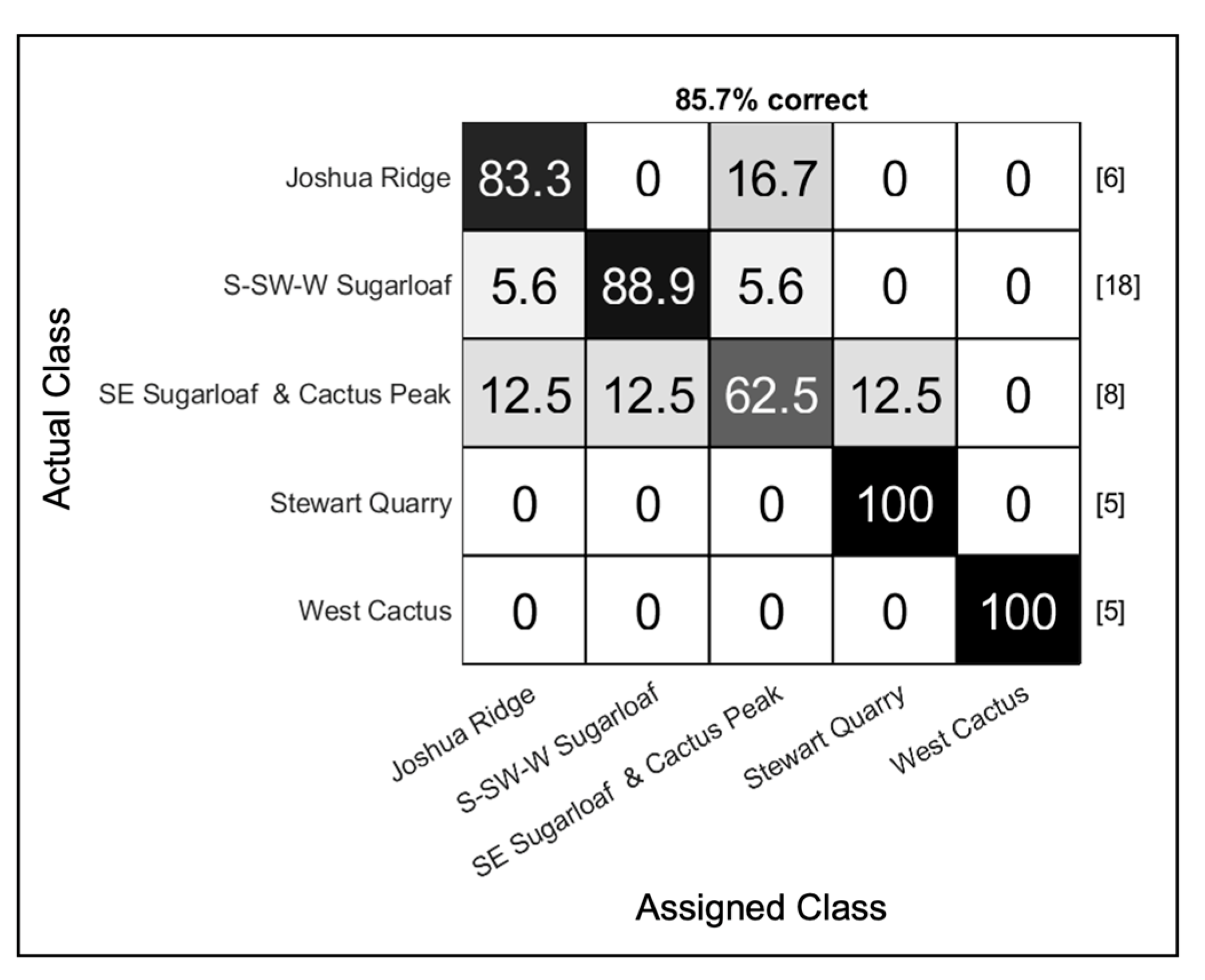
5.1.4. Coso Sub-Sources
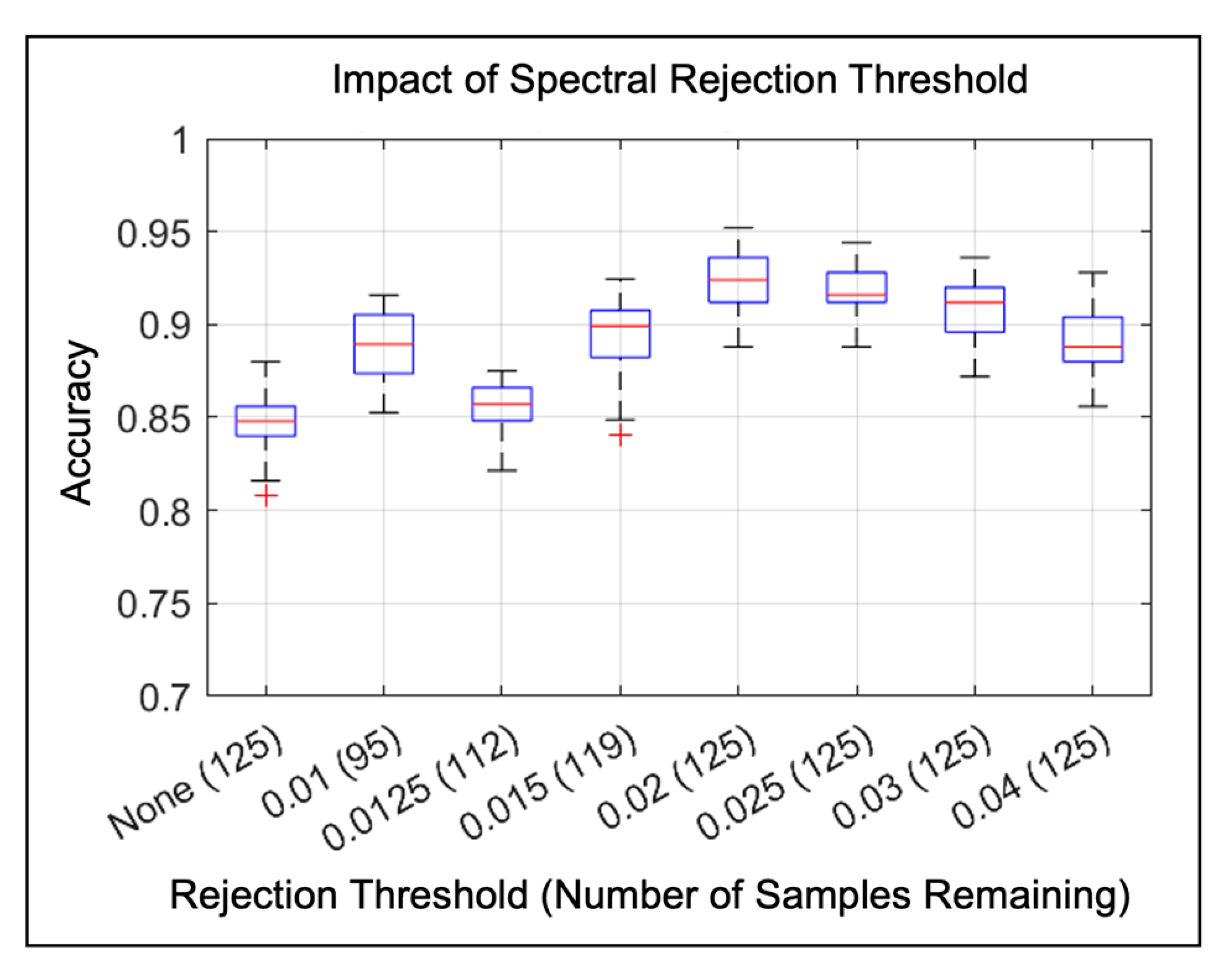
5.1.5. Spectra Rejection Threshold Validation
5.2. Archaeological Obsidian Attribution
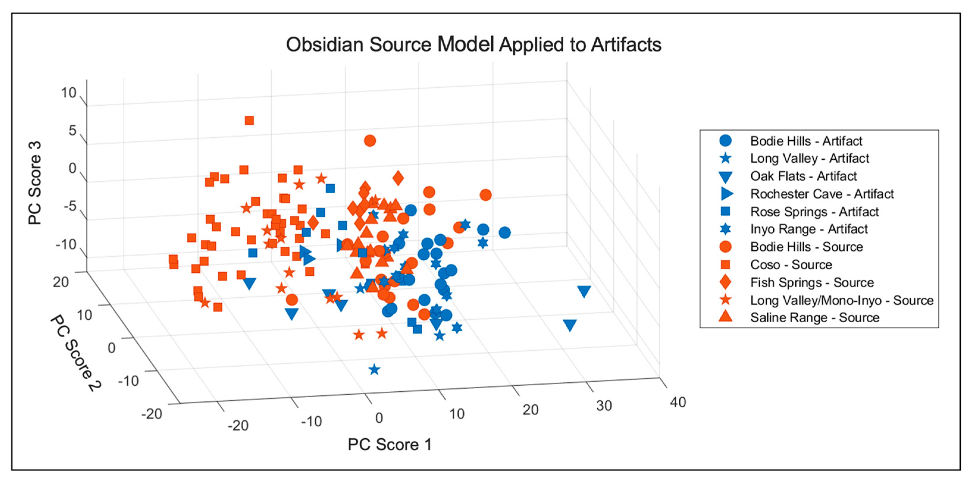
5.2.1. Artifact PCA
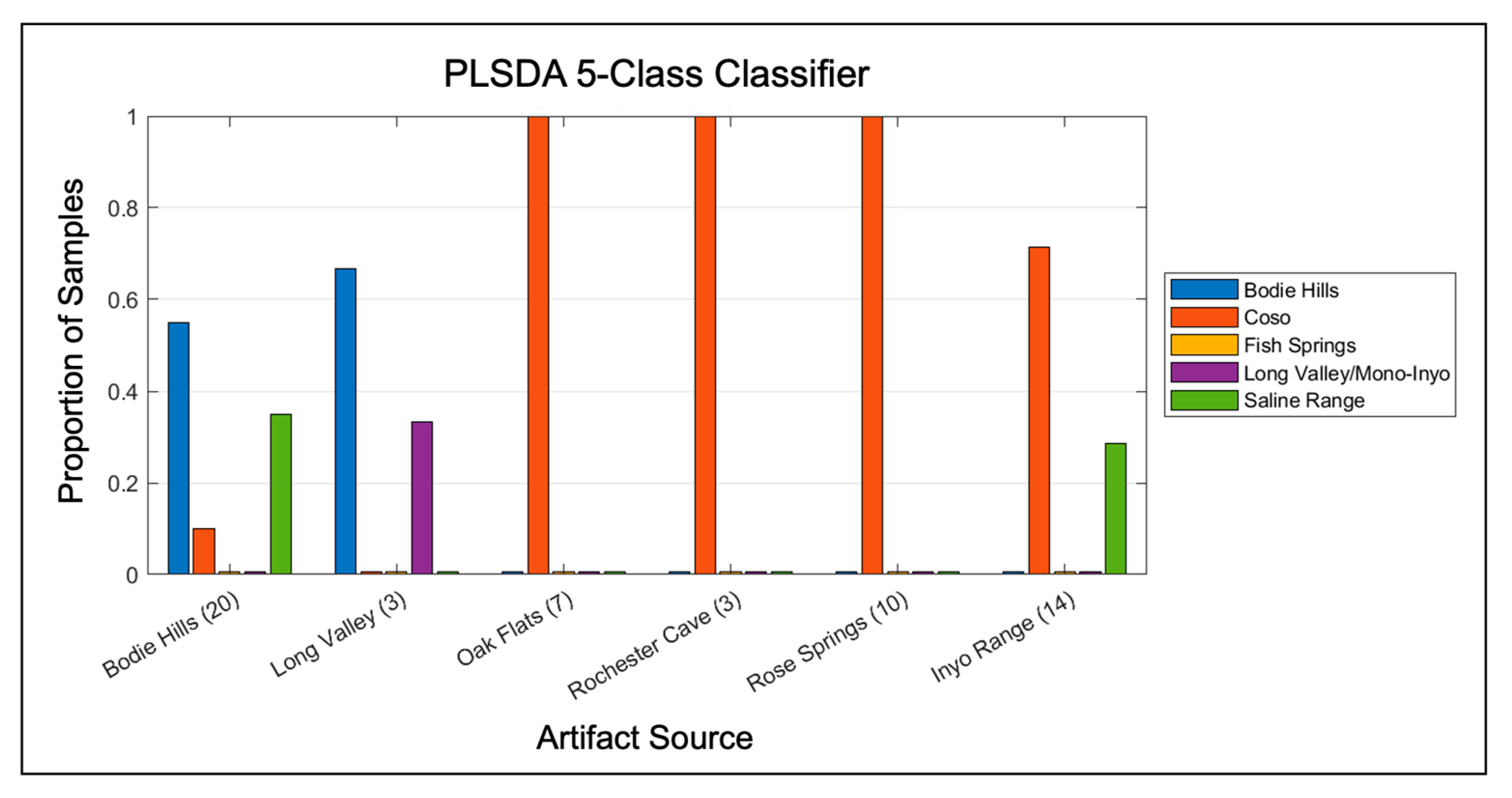
5.2.2. Artifact PLSDA 5-Class Attribution
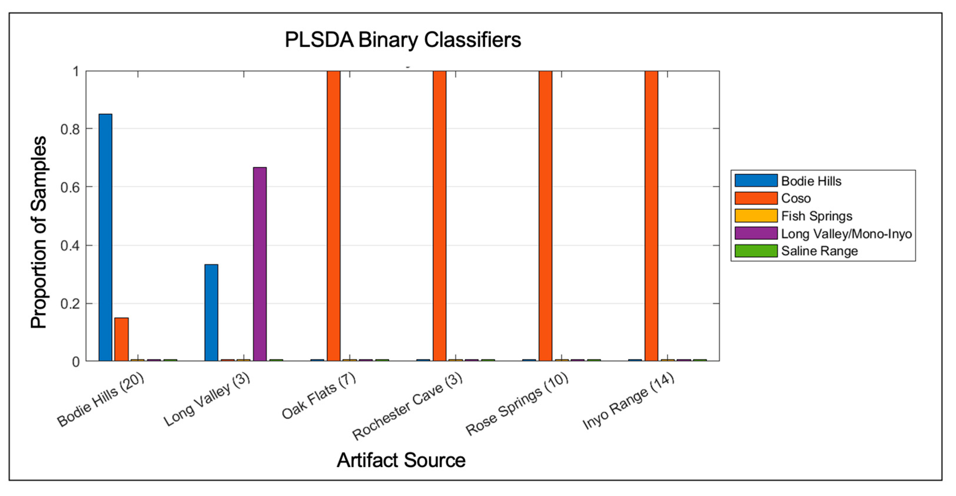
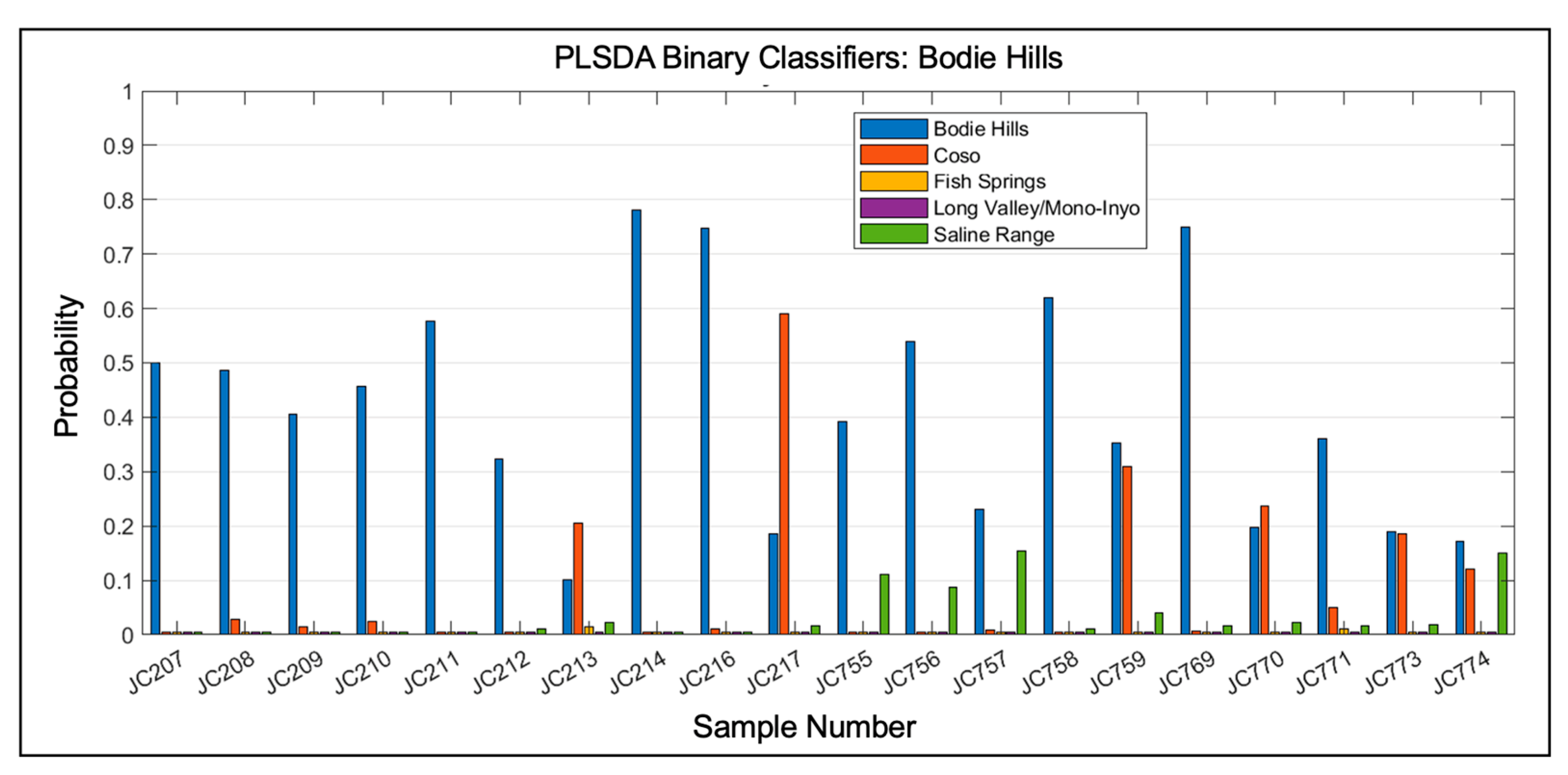
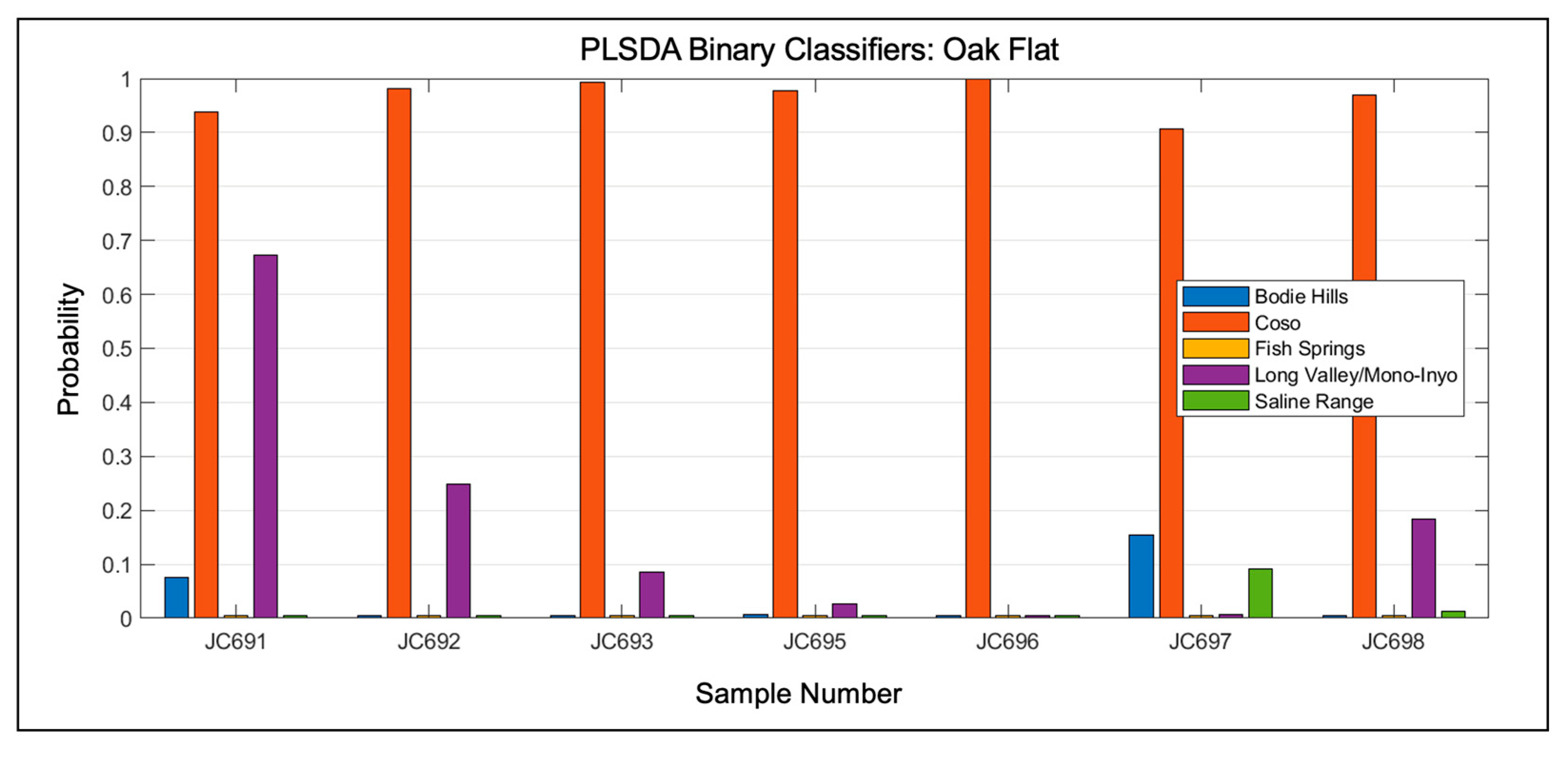
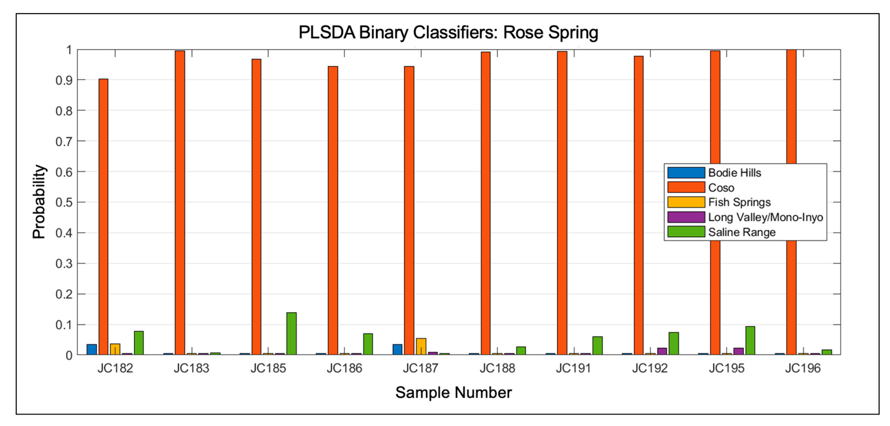
5.2.3. Artifact Single Source Binary Classification
6. Summary and Conclusions
Author Contributions
Funding
Data Availability Statement
Acknowledgments
Conflicts of Interest
References
- Harbottle, G. Chemical characterization in archaeology. In Contexts for Prehistoric Exchange; Ericson, J.E., Earle, T.K., Eds.; Academic Press: New York, NY, USA, 1982; pp. 13–51. [Google Scholar]
- Shackley, M.S. Archaeological Obsidian Studies: Method and Theory. In Advances in Archaeological and Museum Science; Shackley, M.S., Ed.; Plenum Press: New York, NY, USA, 1998; Volume 3, 243p. [Google Scholar]
- Glascock, M.D. A systematic approach to geochemical sourcing of obsidian artifacts. Sci. Cult. 2020, 2, 35–47. [Google Scholar]
- Prochaska, W. The use of geochemical methods to pinpoint the origin of ancient white marbles. Mineral. Petrol. 2023, 117, 401–409. [Google Scholar] [CrossRef] [PubMed]
- Brandl, M.; Martinez, M.M.; Hauzenberger, C.; Filzmoser, P.; Nymoen, P.; Mehler, N. A multi-technique analytical approach to sourcing Scandinavian flint: Provenance of ballast flint from the shipwreck “Leirvigen 1”, Norway. PLoS ONE 2018, 13, e0200647. [Google Scholar] [CrossRef]
- Dilaria, S.; Previato, C.; Bonetto, J.; Secco, M.; Zara, A.; De Luca, R.; Miriello, D. Volcanic pozzolan from the Phlegraean Fields in the structural mortars of the Roman temple of Nora (Sardinia). Heritage 2023, 6, 567–586. [Google Scholar] [CrossRef]
- Su, C.F.; Feng, S.; Singh, J.P.; Yueh, F.Y.; Rigsby, J.T., III; Monts, D.L.; Cook, R.L. Glass composition measurement using laser induced breakdown spectrometry. Glass Technol. 2000, 41, 16–21. [Google Scholar]
- Barnett, C.; Cahoon, E.; Almirall, J.R. Wavelength dependence on the elemental analysis of glass by laser induced breakdown spectroscopy. Spectrochim. Acta Part B At. Spectrosc. 2008, 63, 1016–1023. [Google Scholar] [CrossRef]
- Rodriguez-Celis, E.M.; Gornushkin, I.B.; Heitmann, U.M.; Almirall, J.R.; Smith, B.W.; Winefordner, J.D.; Omenetto, N. Laser induced breakdown spectroscopy as a tool for discrimination of glass for forensic applications. Anal. Bioanal. Chem. 2008, 391, 1961–1968. [Google Scholar] [CrossRef]
- Negre, E.; Motto-Ros, V.; Pelascini, F.; Lauper, S.; Denis, D.; Yu, J. On the performance of laser-induced breakdown spectroscopy for quantitative analysis of minor and trace elements in glass. J. Anal. At. Spectrom. 2015, 30, 417–425. [Google Scholar] [CrossRef]
- Remus, J.J.; Gottfried, J.L.; Harmon, R.S.; Draucker, A.; Baron, D.; Yohe, R. Archaeological applications of LIBS: An example from the Coso Volcanic Field, CA, using advanced statistical signal processing analysis. Appl. Opt. 2010, 49, C120–C131. [Google Scholar] [CrossRef]
- Remus, J.J.; Harmon, R.S.; Hark, R.R.; Haverstock, G.; Baron, D.; Potter, I.K.; Bristol, S.K.; East, L.J. Advanced signal processing analysis of laser-induced breakdown spectroscopy data for the discrimination of obsidian sources. Appl. Opt. 2012, 51, 865–873. [Google Scholar] [CrossRef]
- Hrdlička, A.; Prokeš, L.; Galiová, M.; Novotný, K.; Vitešníková, A.; Helešicová, T.; Kanický, V. Provenance study of volcanic glass using 266–1064 nm orthogonal double pulse laser induced breakdown spectroscopy. Chem. Pap. 2013, 67, 546–555. [Google Scholar] [CrossRef]
- Syvilay, D.; Bousquet, B.; Chapoulie, R.; Orange, M.; Le Bourdonnec, F.X. Advanced statistical analysis of LIBS spectra for the sourcing of obsidian samples. J. Anal. At. Spectrom. 2019, 34, 867–873. [Google Scholar] [CrossRef]
- Hughes, R.E.; Smith, R.L. Archaeology, geology, and geochemistry in obsidian provenance studies. In Effects of Scale on Archaeological and Geoscientific Perspectives; Stein, J.K., Linse, A.R., Eds.; Geological Society America Special Paper 283; Geological Society of America: Boulder, CO, USA, 1993; pp. 79–91. [Google Scholar]
- Fink, J.H.; Manley, C.R. Origin of pumiceous and glassy textures in rhyolite flows and domes. Geol. Soc. Am. Spec. Pap. 1987, 212, 77–88. [Google Scholar]
- Heizer, R.F. Trade and trails. In Handbook of North American Indians: California; Heizer, R.F., Ed.; Smithsonian Institution: Washington, DC, USA, 1978; Volume 8, pp. 690–693. [Google Scholar]
- Jackson, T.L.; Ericson, J.E. Prehistoric exchange systems in California. In Prehistoric Exchange Systems in North America; Johnson, J.K., Baugh, T.G., Ericson, J.E., Eds.; Springer: Boston, MA, USA, 1994; pp. 385–415. [Google Scholar]
- Bettinger, R.L.; Delacorte, M.G.; Jackson, R.J. Visual sourcing of central eastern California obsidians. In Obsidian Studies in the Great Basin; Hughes, R.E., Ed.; Archaeological Research Facility, University of California Berkeley: Berkeley, CA, USA, 1984; Volume 45, pp. 63–78. [Google Scholar]
- Braswell, G.E.; Clark, J.E.; Aoyama, K.; McKillop, H.I.; Glascock, M.D. Determining the geological provenance of obsidian artifacts from the Maya region: A test of the efficacy of visual sourcing. Lat. Am. Antiq. 2000, 11, 269–282. [Google Scholar] [CrossRef]
- Kamber, B.S. Geochemical fingerprinting: 40 years of analytical development and real world applications. Appl. Geochem. 2009, 24, 1074–1086. [Google Scholar] [CrossRef]
- Hoefs, J. Geochemical fingerprints: A critical appraisal. Eur. J. Mineral. 2010, 22, 3–15. [Google Scholar] [CrossRef]
- Harmon, R.S.; Remus, J.; McMillan, N.J.; McManus, C.; Collins, L.; Gottfried, J.L., Jr.; DeLucia, F.C.; Miziolek, A.W. LIBS analysis of geomaterials: Geochemical fingerprinting for the rapid analysis and discrimination of minerals. Appl. Geochem. 2009, 24, 1125–1141. [Google Scholar] [CrossRef]
- Harmon, R.S.; Hark, R.R.; Throckmorton, C.S.; Rankey, E.C.; Wise, M.A.; Somers, A.M.; Collins, L.M. Geochemical fingerprinting by handheld laser-induced breakdown spectroscopy (LIBS). J. Geostand. Geoanal. Res. 2017, 41, 563–584. [Google Scholar] [CrossRef]
- Harmon, R.S.; Lawley, C.J.; Watts, J.; Harraden, C.L.; Somers, A.M.; Hark, R.R. Laser-induced breakdown spectroscopy—An emerging analytical tool for mineral exploration. Minerals 2019, 9, 718. [Google Scholar] [CrossRef]
- Alvey, D.C.; Morton, K.; Harmon, R.S.; Gottfried, J.L.; Remus, J.J.; Collins, L.M.; Wise, M.A. Laser-induced breakdown spectroscopy-based geochemical fingerprinting for the rapid analysis and discrimination of minerals: The example of garnet. Appl. Opt. 2010, 49, C168–C180. [Google Scholar] [CrossRef]
- Hark, R.R.; Remus, J.J.; East, L.J.; Harmon, R.S.; Wise, M.A.; Tansi, B.M.; Shughrue, K.M.; Dunsin, K.S.; Liu, C. Geographical analysis of “conflict minerals” utilizing laser-induced breakdown spectroscopy. Spectrochim. Acta Part B At. Spectrosc. 2012, 74, 131–136. [Google Scholar] [CrossRef]
- Hark, R.R.; Harmon, R.S. Geochemical fingerprinting using LIBS. In Laser Induced Breakdown Spectroscopy—Theory and Applications; Musazzi, S., Perini, U., Eds.; Springer: New York, NY, USA, 2014; pp. 309–348. [Google Scholar]
- Costantini, I.; Veneranda, M.; Prieto-Taboada, N.; De Francesco, A.M.; Castro, K.; Madariaga, J.M.; Arana, G. Combined in situ XRF–LIBS analyses as a novel method to determine the provenance of central Mediterranean obsidians. Eur. Phys. J. Plus 2023, 138, 603. [Google Scholar] [CrossRef]
- Xing, P.; Zhu, Z. Geochemical Fingerprinting Using Laser-Induced Breakdown Spectroscopy. In Laser Induced Breakdown Spectroscopy (LIBS): Concepts, Instrumentation, Data Analysis and Applications; Singh, V.K., Tripathi, D.K., Deguchi, Y., Wang, Z., Eds.; Wiley & Sons: New York, NY, USA, 2023; Volume 33, pp. 683–699. [Google Scholar]
- Hildreth, W.; Moorbath, S. Crustal contributions to arc magmatism in the Andes of central Chile. Contrib. Mineral. Petrol. 1988, 98, 455–489. [Google Scholar] [CrossRef]
- Donnelly-Nolan, J.M. Chemical Analyses of Pre-Holocene Rocks from Medicine Lake Volcano and Vicinity, Northern California; U.S. Geological Survey Open-File Report 2008–1094; U.S. Geological Survey: Reston, VA, USA, 2008; 9p.
- Grove, T.L.; Donnelly-Nolan, J.M. The evolution of young silicic lavas at Medicine Lake Volcano, California: Implications for the origin of compositional gaps in calc-alkaline series lavas. Contrib. Mineral. Petrol. 1986, 92, 281–302. [Google Scholar] [CrossRef]
- Sweetkind, D.S.; Rytuba, J.J.; Langenheim, V.E.; Fleck, R.J. Geology and geochemistry of volcanic centers within the eastern half of the Sonoma volcanic field, northern San Francisco Bay region, California. Geosphere 2011, 7, 629–657. [Google Scholar] [CrossRef]
- Noble, D.C.; Korringa, M.K.; Hedge, C.E.; Riddle, G.O. Highly differentiated subalkaline rhyolite from Glass Mountain, Mono County, California. Geol. Soc. Am. Bull. 1972, 83, 1179–1184. [Google Scholar] [CrossRef]
- Metz, J.M.; Mahood, G.A. Development of the Long Valley, California, magma chamber recorded in precaldera rhyolite lavas of Glass Mountain. Contrib. Mineral. Petrol. 1991, 106, 379–397. [Google Scholar] [CrossRef]
- Bailey, R.A. Eruptive History and Chemical Evolution of the Precaldera and Postcaldera Basalt-Dacite Sequences, Long Valley, California: Implications for Magma Sources, Current Seismic Unrest, and Future Volcanism; U.S. Geological Survey Professional Paper 1692; U.S. Geological Survey: Reston, VA, USA, 2004; 75p.
- Sampson, D.E.; Cameron, K.L. The geochemistry of the Inyo Volcanic Chain: Multiple magma systems in the Long Valley region, eastern California. J. Geophys. Res. 1987, 92, 10403–10421. [Google Scholar] [CrossRef]
- Vogel, T.A.; Eichelberger, J.C.; Younker, L.W.; Schuraytz, B.C.; Horkowitz, J.P.; Stockman, H.W.; Westrich, H.R. Petrology and emplacement dynamics of intrusive and extrusive rhyolites of Obsidian Dome, Inyo Craters Volcanic Chain, eastern California. J. Geophys. Res. Solid Earth 1989, 94, 17937–17956. [Google Scholar] [CrossRef]
- du Bray, E.A.; John, D.A.; Cousens, B.L.; Hayden, L.A.; Vikre, P.G. Geochemistry, petrologic evolution, and ore deposits of the Miocene Bodie Hills Volcanic Field, California and Nevada. Am. Mineral. 2016, 101, 644–677. [Google Scholar] [CrossRef]
- John, D.A.; du Bray, E.A.; Blakely, R.J.; Fleck, R.J.; Vikre, P.G.; Box, S.E.; Moring, B.C. Miocene magmatism in the Bodie Hills volcanic field, California and Nevada: A long-lived eruptive center in the southern segment of the ancestral Cascades arc. Geosphere 2012, 8, 44–97. [Google Scholar] [CrossRef]
- Bacon, C.R.; Macdonald, R.; Smith, R.L.; Baedecker, P.A. Pleistocene high-silica rhyolites of the Coso Volcanic Field, Inyo County, California. J. Geophys. Res. 1981, 86, 10223–10241. [Google Scholar] [CrossRef]
- Parks, G.A.; Tieh, T.T. Identifying the geographical source of artefact obsidian. Nature 1966, 211, 289–290. [Google Scholar] [CrossRef]
- Constantinescu, B.; Bugoi, R.; Sziki, G. Obsidian provenance studies of Transylvania’s Neolithic tools using PIXE, micro-PIXE, and XRF. Nucl. Instrum. Methods Phys. Res. Sect. B Beam Interact. Mater. At. 2002, 189, 373–377. [Google Scholar] [CrossRef]
- Le Bourdonnec, F.-X.; Poupeau, G.; Lugliè, C. SEM–EDS analysis of western Mediterranean obsidians: A new tool for Neolithic provenance studies. Comptes Rendus Geosci. 2006, 338, 1150–1157. [Google Scholar] [CrossRef]
- De Francesco, A.M.; Crisci, G.M.; Bocci, M. Non-destructive analytic method using XRF for determination of provenance of archaeological obsidians from the Mediterranean area: A comparison with traditional XRF methods. Archaeometry 2008, 50, 337–350. [Google Scholar] [CrossRef]
- Poupeau, G.; Le Bourdonnec, F.-X.; Carter, T.; Delerue, S.; Shackley, M.S.; Barrat, J.-X.; Dubernet, S.; Moretto, P.; Calligaro, T.; Milic, M.; et al. The use of SEM-EDS, PIXE and EDXRF for obsidian provenance studies in the Near East: A case study from Neolithic Çatalhöyük (central Anatolia). J. Archaeol. Sci. 2010, 37, 2705–2720. [Google Scholar] [CrossRef]
- Nash, B.P.; Merrick, H.V.; Brown, F.H. Obsidian types from Holocene sites around Lake Turkana, and other localities in northern Kenya. J. Archaeol. Sci. 2011, 38, 1371–1376. [Google Scholar] [CrossRef]
- Nelson, C.A. Geologic Map of the Waucoba Spring Quadrangle, Inyo County; California: U.S. Geological Survey Geologic Quadrangle Map GQ-921; U.S. Geological Survey: Reston, VA, USA, 1971.
- Reepmeyer, C.; Spriggs, M.; Lape, P.; Neri, L.; Ronquillo, W.P.; Simanjuntak, T.; Summerhayes, G.; Tanudirjo, D.; Tiauzon, A. Obsidian sources and distribution systems in Island Southeast Asia: New results and implications from geochemical research using LA-ICPMS. J. Archaeol. Sci. 2011, 38, 2995–3005. [Google Scholar] [CrossRef]
- Ericson, J.E.; Hagan, T.A.; Chesterman, C.W. Prehistoric obsidian sources in California, II: Geologic and geographic aspects. In Advances in Obsidian Glass Studies: Archaeological and Geochemical Perspectives; Taylor, R.E., Ed.; Noyes Press: Park Ridge, NJ, USA, 1976; pp. 218–239. [Google Scholar]
- Ericson, J.E. Exchange and Production Systems in Californian Prehistory: The Results of Hydration Dating and Chemical Characterization of Obsidian Sources; British Archaeological Reports International Series 110; BAR Publishing: Oxford, UK, 1981; 289p. [Google Scholar]
- Craig, N.; Speakman, R.J.; Popelka-Filcoff, R.S.; Glascock, M.D.; Robertson, J.D.; Shackley, M.S.; Aldenderfer, M.S. Comparison of XRF and PXRF for analysis of archaeological obsidian from southern Peru. J. Archaeol. Sci. 2007, 34, 2012–2024. [Google Scholar] [CrossRef]
- Phillips, S.C.; Speakman, R.J. Initial source evaluation of archaeological obsidian from the Kuril Islands of the Russian Far East using portable XRF. J. Archaeol. Sci. 2009, 36, 1256–1263. [Google Scholar] [CrossRef]
- Sheppard, P.; Trichereau, B.; Milicich, C. Pacific obsidian sourcing by portable XRF. Archaeol. Ocean. 2010, 45, 21–30. [Google Scholar] [CrossRef]
- Frahm, E. Characterizing obsidian sources with portable XRF: Accuracy, reproducibility, and field relationships in a case study from Armenia. J. Archaeol. Sci. 2014, 49, 105–125. [Google Scholar] [CrossRef]
- Tykot, R.H. Using nondestructive portable X-ray fluorescence spectrometers on stone, ceramics, metals, and other materials in museums: Advantages and limitations. Appl. Spectrosc. 2016, 70, 42–56. [Google Scholar] [CrossRef]
- Frahm, E.; Tryon, C.A. Later Stone Age toolstone acquisition in the Central Rift Valley of Kenya: Portable XRF of Eburran obsidian artifacts from Leakey’s excavations at Gamble’s Cave II. J. Archaeol. Sci. 2018, 18, 475–486. [Google Scholar] [CrossRef]
- Jack, R.N.; Carmichael, I.S.E. The chemical fingerprinting of acid volcanic rocks. Calif. Div. Mines Geol. Spec. Rep. 1969, 100, 17–32. [Google Scholar]
- Jack, R.N. Prehistoric obsidian in California I: Geochemical aspects. In Advances in Obsidian Glass Studies: Archaeological and Geochemical Perspectives; Taylor, R.E., Ed.; Noyes Press: Park Ridge, NJ, USA, 1976; pp. 183–217. [Google Scholar]
- Bowman, H.R.; Asaro, F.; Perlman, I. Composition variations in obsidian sources and the archaeological implications. Archaeometry 1973, 15, 123–127. [Google Scholar] [CrossRef]
- Shackley, M.S. Intersource and intrasource geochemical variability in two newly discovered archaeological obsidian sources in the southern Great Basin. J. Calif. Great Basin Anthropol. 1994, 16, 118–129. [Google Scholar]
- Hughes, R.E. The Coso Volcanic Field reexamined: Implications for obsidian sourcing and hydration dating research. Geoarchaeology 1988, 3, 253–265. [Google Scholar] [CrossRef]
- Northwest Research Obsidian Studies Laboratory. United States and Canada Obsidian Source Catalog. 2023. Available online: https://www.sourcecatalog.com/ca/s_ca.html (accessed on 20 August 2023).
- Silliman, S.W. Obsidian studies and the archaeology of 19th-century California. J. Field Archaeol. 2005, 30, 75–94. [Google Scholar] [CrossRef]
- Dolan, S.G.; Shackley, M.S.; Wyckoff, D.G.; Skinner, C.E. Long-distance conveyance of California obsidian at the Hayhurst lithic cache site (34ML168) in Oklahoma. Plains Anthropol. 2017, 62, 1–19. [Google Scholar] [CrossRef]
- Hughes, R.E. Obsidian studies in California archaeology. Quat. Int. 2018, 482, 67–82. [Google Scholar] [CrossRef]
- Sutton, M.Q.; Des Lauriers, M.R. Emerging Patterns in obsidian usage in the southern San Joaquin Valley, California. Pac. Coast Archaeol. Soc. Q. 2002, 38, 2–18. [Google Scholar]
- Fredrickson, D.A. Cultural diversity in early central California: A view from the North Coast Ranges. J. Calif. Anthropol. 1974, 1, 41–53. [Google Scholar]
- Eerkens, J.W.; Spurling, A.M. Obsidian acquisition and exchange networks: A diachronic perspective on households in the Owens Valley. J. Calif. Great Basin Anthropol. 2008, 28, 111–126. [Google Scholar]
- Hall, M.C. Late Holocene Hunter-Gatherers and Volcanism in the Long Valley-Mono Basin Region: Prehistoric Culture Change in the Eastern Sierra Nevada. Ph.D. Thesis, University of California–Riverside, Los Angeles, CA, USA, 1983. Unpublished. [Google Scholar]
- Panich, L.M.; Griffin, B.; Schneider, T.D. Native acquisition of obsidian in colonial-era central California: Implications from Mission San José. J. Anthropol. Archaeol. 2018, 50, 1–11. [Google Scholar] [CrossRef]
- Ericson, J.E. Egalitarian exchange systems in California: A preliminary view. In Exchange Systems in Prehistory; Earle, T.K., Ericson, J.E., Eds.; Academic Press: New York, NY, USA, 1977; pp. 109–126. [Google Scholar]
- Bettinger, R.L. Aboriginal exchange and territoriality in Owens Valley, California. In Contexts for Prehistoric Exchange; Ericson, J.E., Earle, T.K., Eds.; Academic Press: New York, NY, USA, 1982; pp. 103–128. [Google Scholar]
- Hughes, R.E.; Bettinger, R.L. Obsidian and prehistoric sociocultural systems in California. In Exploring the Limits: Frontiers and Boundaries in Prehistory; DeAtley, S.P., Findlow, F.J., Eds.; British Archaeological Reports, International Series 223; BAR Publishing: Oxford, UK, 1984; pp. 153–172. [Google Scholar]
- Basgall, M.E. Obsidian acquisition and use in prehistoric central eastern California: A preliminary assessment. Current Directions in California Obsidian Studies. Contrib. Univ. Calif. Archaeol. Res. Facil. 1989, 48, 111–126. [Google Scholar]
- Eerkens, J.W.; Spurling, A.M.; Gras, M.A. Measuring prehistoric mobility strategies based on obsidian geochemical and technological signatures in the Owens Valley, California. J. Archaeol. Sci. 2008, 35, 668–680. [Google Scholar] [CrossRef]
- Brady, R.T. Obsidian source distribution and prehistoric settlement patterns at Mono Lake, Eastern California. J. Calif. Great Basin Anthropol. 2011, 31, 3–24. [Google Scholar]
- Bouey, P.D.; Basgall, M.E. Trans-Sierran exchange in prehistoric California: The concept of economic articulation. Obsidian Stud. Great Basin 1984, 45, 135–172. [Google Scholar]
- Roper-Wickstrom, C.K. Spatial and temporal characteristics of high altitude site patterning in the southern Sierra Nevada. In There Grows a Green Tree: Papers in Honor of David; Fredrickson, A., White, G., Mikkelsen, P., Hildebrandt, W.T., Basgall, M.E., Eds.; UC–Davis Center for Archaeological Research: Davis, CA, USA, 1993; Volume 11, pp. 285–301. [Google Scholar]
- McGuire, K.R. Test Excavations at CA-FRE-61, Fresno County, California; UC–Bakersfield Museum of Anthropology Occasional Papers in Anthropology: Bakersfield, CA, USA, 1995; Volume 5, 138p. [Google Scholar]
- Hughes, R.E.; True, D.L. Perspectives on the distribution of obsidians in San Diego County, California. N. Am. Archaeol. 1986, 6, 325–339. [Google Scholar] [CrossRef]
- Hughes, R.E.; Bennyhoff, J.A. Early Trade. In Handbook of North American Indians: Great Basin; d’Azevedo, W.L., Ed.; Smithsonian Institution Press: Washington, DC, USA, 1986; Volume 11, pp. 238–255. [Google Scholar]
- Donnelly-Nolan, J.M.; Champion, D.E.; Miller, C.D.; Grove, T.L.; Trimble, D.A. Post-11,000-year volcanism at Medicine Lake Volcano, Cascade Range, northern California. J. Geophys. Res. Solid Earth 1990, 95, 19693–19704. [Google Scholar] [CrossRef]
- Donnelly-Nolan, J.M.; Champion, D.E.; Grove, T.L. Late Holocene Volcanism at Medicine Lake Volcano, Northern California Cascades; U.S. Geological Survey Professional Paper 1822; U.S. Geological Survey: Reston, VA, USA, 2016; 59p.
- Davis, J.T. Trade Routes and Economic Exchange among the Indians of California; Reports of the University California Archaeological Survey No. 54; The University California Archaeological Survey: Berkeley, CA, USA, 1961; 73p. [Google Scholar]
- Hughes, R.E. Age and exploitation of obsidian from the Medicine Lake Highland, California. J. Archaeol. Sci. 1982, 9, 173–185. [Google Scholar] [CrossRef]
- Delacorte, M.G.; Basgall, M.E. Great Basin-California/Plateau interactions along the western front. In Meeting at the Margins: Prehistoric Cultural Interactions in the Intermountain West; Rhode, D., Ed.; University of Utah Press: Salt Lake City, UT, USA, 2012; pp. 65–91. [Google Scholar]
- Fox, K.F. Tectonic setting of Late Miocene, Pliocene, and Pleistocene rocks north of San Francisco, California; U.S. Geological Survey Professional Paper 1239; U.S. Geological Survey: Reston, VA, USA, 1983; 33p.
- Higgins, C.T. Geology of Annadel State Park, Sonoma County. Calif. Geol. 1983, 36, 235–241. [Google Scholar]
- Fox, K.F.; Sims, J.D.; Bartlow, J.A.; Helley, E.J. Preliminary Geologic Map of Eastern Sonoma County and Western Napa County, California; U.S. Geological Survey Miscellaneous Field Studies Map MF-483; U.S. Geological Survey: Reston, VA, USA, 1973; 5p.
- Jackson, T.L. Late prehistoric obsidian production and exchange in the North Coast Ranges, California. In Current Directions in California Obsidian Studies; Hughes, R.E., Ed.; University of California Archaeological Research Facility Publication: Berkeley, CA, USA, 1989; Volume 48, pp. 79–94. [Google Scholar]
- Bergthold, J.C. The Prehistoric Settlements and Trade Models in the Santa Clara Valley. Master’s Thesis, California State University, San Francisco, CA, USA, 1982. Unpublished. [Google Scholar]
- Milliken, R.T.; Fitzgerald, R.T.; Hylkema, M.G.; Groza, R.; Origer, T.; Bieling, D.G.; Leventhal, A.; Wiberg, R.S.; Gottsfield, A.; Gillette, D.; et al. Punctuated culture change in the San Francisco Bay area. In California Prehistory: Colonization, Culture, and Complexity; Jones, T.L., Klar, K.A., Eds.; Altamira Press: Lanham, MD, USA, 2007; pp. 99–124. [Google Scholar]
- King, J.; Hildebrandt, W.R.; Rosenthal, J.S. Evaluating alternative models for the conveyance of Bodie Hills obsidian into central California. In Perspectives on Prehistoric Trade and Exchange in California and the Great Basin; Hughes, R.E., Ed.; University of Utah Press: Salt Lake City, UT, USA, 2011; pp. 148–170. [Google Scholar]
- Jackson, T.L. Late Prehistoric Obsidian Exchange in Central California. Ph.D. Thesis, Stanford University, Stanford, CA, USA, 1986. Unpublished. [Google Scholar]
- Shackley, M.S. Source Provenance of Obsidian Artifacts from CA-SMA-113, West-Central California; Contributions of the University of California Archaeological Research Facility: Berkeley, CA, USA, 2011; 13p. [Google Scholar]
- Kleinhampl, F.J.; Davis, W.E.; Silberman, M.L.; Chesterman, C.W.; Chapman, R.H.; Gray, C.H. Aeromagnetic and Limited Gravity Studies and Generalized Geology of the Bodie Hills Region, Nevada and California; U.S. Geological Survey Bulletin; U.S. Geological Survey: Reston, VA, USA, 1975; Volume 1384, 38p.
- Nelson, C.A.; Hall, C.A., Jr.; Ernst, W.G. Geologic history of the White-Inyo Range. In Natural History of the White Inyo-Range, Eastern California; Hall, C.A., Ed.; University of California Press: Berkeley, CA, USA, 1991; pp. 42–74. [Google Scholar]
- Chesterman, C.W.; Chapman, R.H.; Gray, C.H. Geology and Ore Deposits of the Bodie Mining District, Mono County, California; California Division Mines Geological Bulletin; California Dept. of Conservation, Division of Mines and Geology: Sacramento, CA, USA, 1986; Volume 206, 86p. [Google Scholar]
- Meighan, C.W. Notes on the Archaeology of Mono County. Univ. Calif. Archaeol. Surv. Rep. 1955, 28, 6–28. [Google Scholar]
- Eerkens, J.W.; Glascock, M.D. Northern Fish Lake Valley and the volcanic tablelands of Owens Valley: Two minor sources of obsidian in the western Great Basin. J. Calif. Great Basin Anthropol. 2000, 22, 331–342. [Google Scholar]
- Fleck, R.J.; du Bray, E.A.; John, D.A.; Vikre, P.G.; Cosca, M.A.; Snee, L.W.; Box, S.E. Geochronology of Cenozoic Rocks in the Bodie Hills, California and Nevada; US Department of the Interior, U.S. Geological Survey Data Series 916; U.S. Geological Survey: Reston, VA, USA, 2015; 26p.
- Al-Rawi, Y.T. Cenozoic History of the Northern Part of Mono Basin, California and Nevada. Ph.D. Thesis, University of California, Berkeley, CA, USA, 1970. [Google Scholar]
- Halford, F.K. The Coleville and Bodie Hills NRCS Soil Inventory, Walker and Bridgeport, California: A Reevaluation of the Bodie Hills Obsidian Source and Its Spatial and Chronological Use; Report on File; BLM Bishop Field Office: Bishop, Ca, USA, 2008; 101p. [Google Scholar]
- Halford, F.K. Archaeology and Environment on the Dry Lakes Plateau, Bodie Hills, California: Hunter-Gatherer Coping Strategies for Holocene Environmental Variability. Mater’s Thesis, University of Nevada, Reno, NV, USA, 1998. Unpublished. [Google Scholar]
- Halford, F.K. Evaluation of CA–MNO-3125/H and CA–MNO-3126 for the Bridgeport Indian Colony 40 Acre Land Sale; Cultural Resource Project: CA–170–00–10; Report on File; Bureau of Land Management, Bishop Field Office: Bishop, CA, USA, 2000. [Google Scholar]
- Halford, F.K. New Evidence for Acquisition and Production of Bodie Hills Obsidian. Soc. Calif. Archaeol. Newsl. 2001, 35, 32–37. [Google Scholar]
- Singer, C.A.; Ericson, J.E. Quarry analysis at Bodie Hills, Mono County, California: A case study. In Exchange Systems in Prehistory; Earle, T., Ericson, J., Eds.; Academic Press: New York, NY, USA, 1977; pp. 171–188. [Google Scholar]
- Heizer, R.F. Studying the Windmiller culture. In Archaeological Researches in Retrospect; Willey, G.R., Ed.; Winthrop: Cambridge, UK, 1974; pp. 177–204. [Google Scholar]
- Rosenthal, J.S. The Prehistory of the Sonora Region: Archaeological and Geoarchaeological Investigations for the Stage I of the East Sonora Bypass Project, State Route 108, Tuolumne County, California; Draft Report; California Department of Transportation, District 10: Stockton, CA, USA, 2006. [Google Scholar]
- Hildreth, W. Volcanological perspectives on Long Valley, Mammoth Mountain and Mono Craters: Several contiguous but discrete systems. J. Volcanol. Geotherm. Res. 2004, 136, 169–198. [Google Scholar]
- Bailey, R.A. Geologic Map of the Long Valley Caldea, Mono-Inyo Craters Volcanic Chain, and Vicinity; US Geological Survey Miscellaneous Investigation Series, Map I–1933; U.S. Geological Survey: Reston, VA, USA, 1989.
- Hildreth, W.; Fierstein, J. Geologic Field-Trip Guide to Long Valley Caldera; California: U.S. Geological Survey Scientific Investigations Report 2017–5022–L; U.S. Geological Survey: Reston, VA, USA, 2017.
- Miller, C.D. Holocene eruptions at the Inyo volcanic chain, California: Implications for possible eruptions in Long Valley. Geology 1985, 13, 14–17. [Google Scholar] [CrossRef]
- Woolfenden, W.B. Historical ecology and the human dimension in ecosystem management. In Draft Region 5 Ecosystem Management Guidebook; U.S. Forest Service, Pacific Southwest Region: Berkeley, CA, USA, 1994; Volume 2, pp. 41–45. [Google Scholar]
- Moratto, M.J. A Study of Prehistory in the Southern Sierra Nevada Foothills. Ph.D. Thesis, University of Oregon–Eugene: Eugene, OR, USA, 1972. Unpublished. [Google Scholar]
- Hughes, R.E. Intrasource chemical variability of artefact-quality obsidians from the Casa Diablo area, California. J. Archaeol. Sci. 1994, 21, 263–271. [Google Scholar] [CrossRef]
- Nelson, C.A. Geologic Map of the Waucoba Mountain Quadrangle, Inyo County; California: U.S. Geological Survey Geologic Quadrangle Map GQ-0528; U.S. Geological Survey: Reston, VA, USA, 1966.
- Elliott, G.S.; Wrucke, C.T.; Nedell, S.S. K-Ar ages of Late Cenozoic volcanic rocks from the northern Death Valley region. Isochron West 1984, 40, 3–7. [Google Scholar]
- Blakely, R.J.; McKee, E.H. Subsurface structural features of the Saline Range and adjacent regions of eastern California as interpreted from isostatic residual gravity anomalies. Geology 1985, 13, 781–785. [Google Scholar] [CrossRef]
- Ross, D.C. Pegmatitic Trachyandesite Plugs and Associated Volcanic Rocks in the Saline Range-Inyo Mountains Region; California: U.S. Geological Survey Professional Paper 614-D; U.S. Geological Survey: Reston, VA, USA, 1970; pp. 1–29.
- Burchfiel, B.C. Geologic Map and Sections of the Dry Mountain Quadrangle, Inyo County; Special Report 99; California Division of Mines and Geology: Sacramento, CA, USA, 1969. [Google Scholar]
- Norwood, R.H.; Bull, C.S.; Quinn, R. A Cultural Resource Overview of the Eureka, Saline, Panamint, and Darwin Region, East Central California; Bureau of Land Management: Riverside, CA, USA, 1980; 219p. [Google Scholar]
- Johnson, L.; Wagner, D.L. Obsidian Quarry Sites in the Saline Range. In Proceedings of the Inyo County, California: Great Basin Anthropological Conference Abstracts 35-4, Bend, OR, USA, 8–11 April 1998. [Google Scholar]
- Burton, J.F. The Archeology of Somewhere: Archeological Testing along U.S. Highway 395 Manzanar National Historic Site, California; U.S. National Park Service Western Archeological Conservation Center Publications in Anthropology: Tucson, AZ, USA, 1998; Volume 72, 238p. [Google Scholar]
- Johnson, L.; Wagner, D.L.; Skinner, C.E. Geochemistry of archeological obsidian sources in the Saline Range, Death Valley National Park, California. In Proceedings of the Conference on Status of Geologic Research and Mapping, Death Valley National Park; Slate, Reston, VA, USA, 9–11 April 1999; U.S. Geological Survey Open–File Report 99–153. U.S. Geological Survey: Reston, VA, USA, 1999; pp. 118–120. [Google Scholar]
- Haverstock, G.J. Prehistoric High Elevation Resource Utilization of the Inyo Mountains; Report on File; Bureau of Land Management, Bishop Field Office: Bishop, CA, USA, 2010. [Google Scholar]
- Blondes, M.S.; Reiners, P.W.; Ducea, M.N.; Singer, B.S.; Chesley, J. Temporal–compositional trends over short and long time-scales in basalts of the Big Pine Volcanic Field, California. Earth Planet. Sci. Lett. 2008, 269, 140–154. [Google Scholar]
- Macdonald, R.; Smith, R.L.; Thomas, J.E. Chemistry of the Subalkalic Silicic Obsidians; U.S. Geological Survey Professional Paper 1523; U.S. Geological Survey: Reston, VA, USA, 1992; 214p.
- Cox, A.; Doell, R.R.; Dalrymple, G.B. Geomagnetic polarity epochs and Pleistocene geochronometry. Nature 1963, 198, 1049–1051. [Google Scholar] [CrossRef]
- Lidzbarski, M.I.; Vazquez, J.A. High-Silica Rhyolite Magmatism in the Big Pine Volcanic Field, Eastern California. In Proceedings of the AGU Fall Meeting Abstract V51C-0720, Washington, DC, USA, 10–14 December 2007. [Google Scholar]
- Steward, J.S. Ethnography of the Owens Valley Paiute. Univ. Calif. Publ. Am. Archaeol. Ethnol. 1933, 33, 233–350. [Google Scholar]
- Norman, L.A.; Stewart, R.M. Mines and Mineral Resources of Inyo County. Calif. J. Mines Geol. 1951, 47, 17–223. [Google Scholar]
- Stevens, N. Prehistoric Use of the Alpine Sierra Nevada: Archaeological Investigations at Taboose Pass, Kings Canyon National Park, California. Master’s Thesis, California State University–Sacramento, Long Beach, CA, USA, 2002. [Google Scholar]
- Johnson, L. Prehistoric Acquisition and Use of Obsidian in Death Valley National Park. In Proceedings of the 6th Death Valley Conference on History and Prehistory, Furnace Creek, CA, USA, 7–10 February 2002. [Google Scholar]
- Duffield, W.A.; Bacon, C.R.; Dalrymple, G.B. Late Cenozoic volcanism, geochronology, and structure of the Coso range, Inyo County, California. J. Geophys. Res. Solid Earth 1980, 85, 2381–2404. [Google Scholar]
- Novak, S.W.; Bacon, C.R. Pliocene Volcanic Rocks of the Coso Range, Inyo County, California; U.S. Geological Survey Professional Paper 1383; U.S. Geological Survey: Reston, VA, USA, 1986; 44p.
- Duffield, W.A.; Smith, G.I. Pleistocene history of volcanism and the Owens River near Little Lake, California. J. Res. U.S. Geol. Surv. 1978, 6, 395–408. [Google Scholar]
- Bacon, C.R.; Duffield, W.A.; Nakamura, K. Distribution of Quaternary rhyolite domes of the Coso Range, California: Implications for extent of the geothermal anomaly. J. Geophys. Res. 1980, 85, 2425–2433. [Google Scholar]
- Stevenson, C.M.; Scheetz, B.E. Induced hydration rate development of obsidians from the Coso Volcanic Field: A comparison of experimental procedures. Current Directions in California Obsidian Studies. Contrib. Univ. Calif. Archaeol. Res. Facil. 1989, 48, 23–30. [Google Scholar]
- Bouey, P.D. Recognizing the limits of archaeological applications of non-destructive energy-dispersive X-ray fluorescence analysis of obsidians. MRS Online Proc. Libr. 1990, 185, 309–320. [Google Scholar] [CrossRef]
- Eerkens, J.W.; Rosenthal, J.S. Are obsidian subsources meaningful units of analysis?: Temporal and spatial patterning of subsources in the Coso Volcanic Field, Southeastern California. J. Archaeol. Sci. 2004, 31, 21–29. [Google Scholar] [CrossRef]
- Ericson, J.E.; Glascock, M.D. Subsource characterization: Obsidian utilization of subsources of the Coso Volcanic Field, Coso Junction, California, USA. Geoarchaeology 2004, 19, 779–805. [Google Scholar]
- Draucker, A.C. Geochemical Characterization of Obsidian Sub-Sources from the Coso Range, California Using Laser Ablation Inductively Coupled Plasma Mass Spectrometry as a Tool for Archaeological Investigations. Master’s Thesis, California State University–Bakersfield, Long Beach, CA, USA, 2007. Unpublished. [Google Scholar]
- Farmer, M. An obsidian quarry near Coso Hot Springs. Masterkey J. Southwest Mus. 1937, 11, 7–10. [Google Scholar]
- Heizer, F.; Treganza, A.E. Mines and Quarries of the Indians of California. Calif. Div. Mines Geol. Rep. 1944, 40, 291–359. [Google Scholar]
- Harrington, M.R. A Colossal Quarry. Masterkey J. Southwest Mus. 1951, 25, 15–18. [Google Scholar]
- Yohe, R.M. The introduction of the bow and arrow and Lithic resource use at Rose Spring (CA–INY–372). J. Calif. Great Basin Anthropol. 1998, 20, 26–52. [Google Scholar]
- Lanning, E.P. Archeology of the Rose Spring site. Univ. Calif. Publ. Am. Archaeol. Ethnol. 1963, 49, 237–336. [Google Scholar]
- Garfinkel, A.P. Rose Spring Point Chronology and Numic Population Movements in Eastern California. Pac. Coast Archaeol. Soc. Q. 2007, 43, 42–49. [Google Scholar]
- Schroth, A.; Yohe, R.M. Obsidian use and technological change in Rose Valley: Conclusions based on the analysis of debitage from two sites. Lithic Technol. 2001, 26, 50–70. [Google Scholar]
- Haarklau, L.; Johnson, L.; Wagner, D.L. Fingerprints in the Great Basin: The Nellis Air Force Base Regional Obsidian Sourcing Study; Prewitt & Associates Inc.: Austin, TX, USA, 2005; 152p. [Google Scholar]
- Horne, S.P. The Inland Chumash: Ethnography, Ethnohistory, and Archaeology. Ph.D. Thesis, University of California–Santa Barbara, Los Angeles, CA, USA, 1981. Unpublished. [Google Scholar]
- Draucker, E.L. Archaeological Investigations at the Oak Flat Site (CA-SBA-3931) Santa Barbara County, California. Master’s Thesis, California State University–Bakersfield, Long Beach, CA, USA, 2014. Unpublished. [Google Scholar]
- Mardia, K.V.; Kent, J.T.; Bibby, J.M. Multivariate Analysis; Academic Press: New York, NY, USA, 1979; 521p. [Google Scholar]
- Geladi, P. Chemometrics in spectroscopy. Part 1. Classical chemometrics. Spectrochim. Acta B At. Spectrosc. 2003, 58, 767–782. [Google Scholar] [CrossRef]
- Harmon, R.S.; Throckmorton, C.S.; Hark, R.R.; Gottfried, J.L.; Wörner, G.; Harpp, K.; Collins, L.M. Discriminating volcanic centers with handheld laser-induced breakdown spectroscopy (LIBS). J. Archaeol. Sci. 2018, 98, 112–126. [Google Scholar] [CrossRef]
- Pearson, R.K.; Neuvo, Y.; Astola, J.; Gabbouj, M. The class of generalized Hampel filters. In Proceedings of the 23rd European Signal Processing Conference (EUSIPCO), Nice, France; 2015; pp. 2501–2505. [Google Scholar]
- Wold, S.; Esbensen, K.; Geladi, P. Principal component analysis. Chemom. Intell. Lab. Syst. 1987, 2, 37–52. [Google Scholar] [CrossRef]
- Ståhle, L.; Wold, S. Partial least squares analysis with cross-validation for the two-class problem: A monte carlo study. J. Chemom. 1987, 1, 185–196. [Google Scholar] [CrossRef]
- Brereton, R.G.; Lloyd, G.R. Partial least squares discriminant analysis: Taking the magic away. J. Chemom. 2014, 28, 213–225. [Google Scholar] [CrossRef]
- Mehmood, T.; Liland, K.H.; Snipen, L.; Sæbø, S. A review of variable selection methods in partial least squares regression. Chemom. Intell. Lab. Syst. 2012, 118, 62–69. [Google Scholar] [CrossRef]
- Krishnan, A.; Williams, L.J.; McIntosh, A.R.; Hervé Abdi, H. Partial least squares (PLS) methods for neuroimaging: A tutorial and review. Neuroimage 2011, 56, 455–475. [Google Scholar] [CrossRef]
- de Jong, S. SIMPLS: An alternative approach to partial least squares regression. Chemom. Intell. Lab. Syst. 1993, 18, 251–263. [Google Scholar] [CrossRef]
- Hughes, R.E. Determining the geologic provenance of tiny obsidian flakes in archaeology using nondestructive EDXRF. Am. Lab. 2010, 42, 27–31. [Google Scholar]
- Panich, L.M. Beyond the colonial curtain: Investigating indigenous use of obsidian in Spanish California through the pXRF analysis of artifacts from Mission Santa Clara. J. Archaeol. Sci. Rep. 2016, 5, 521–530. [Google Scholar] [CrossRef]
- Fürnkranz, J. Round robin classification. J. Mach. Learn. Res. 2002, 2, 721–747. [Google Scholar]
- Rifkin, R.; Klautau, A. In defense of one-vs-all classification. J. Mach. Learn. Res. 2004, 5, 101–141. [Google Scholar]
- Platt, J. Probabilistic outputs for support vector machines and comparisons to regularized likelihood methods. Adv. Large Margin Classif. 1999, 10, 61–74. [Google Scholar]
- Niculescu-Mizil, A.; Caruana, R. Predicting good probabilities with supervised learning. In Proceedings of the 22nd International Conference on Machine Learning, Bonn, Germany, 7–11 August 2005; pp. 625–632. [Google Scholar]
- Rogers, A.K.; Yohe, R.M. Recent Advances in Obsidian Hydration Dating. Soc. Calif. Arch. Proc. 2022, 35, 187–196. Available online: https://drive.google.com/file/d/1eK8TdGFViZRnv_w29t9D6N_LS187PngD/view (accessed on 20 August 2023).
- Shackley, M.S. Obsidian: Geology and Archaeology in the North American Southwest; University of Arizona Press: Tucson, AZ, USA, 2005; 246p. [Google Scholar]
- Eerkens, J.W.; Ferguson, J.R.; Glascock, M.D.; Skinner, C.E.; Waechter, S.A. Reduction strategies and geochemical characterization of lithic assemblages: A comparison of three case studies from western North America. Am. Antiq. 2007, 72, 585–597. [Google Scholar] [CrossRef]
- Speakman, R.J.; Neff, H. (Eds.) Laser Ablation ICP-MS in Archaeological Research; University of New Mexico Press: Albuquerque, NM, USA, 2005; 208p. [Google Scholar]


| Obsidian Source/Locality | SiO2 | TiO2 | Al2O3 | MgO | CaO | Na2O | K2O | Ba | Rb | Sr | Zr | Reference |
|---|---|---|---|---|---|---|---|---|---|---|---|---|
| Medicine Lake Highlands | 72.20 | 0.03 | 12.50 | 0.06 | 0.40 | 4.23 | 4.47 | 35 | 147 | 13 | 147 | [32] |
| Cougar Butte | 75.40 | 0.20 | 13.50 | 0.24 | 0.85 | 3.89 | 4.64 | 765 | 134 | 81 | 183 | [32] |
| Grasshopper Flat | 75.00 | 0.24 | 13.50 | 0.36 | 0.91 | 3.82 | 4.80 | 765 | 148 | 84 | 214 | [32] |
| Little Sand Butte | 73.00 | 0.27 | 13.90 | 0.35 | 1.25 | 4.01 | 4.33 | 865 | 154 | 115 | 230 | [33] |
| Glass Mountain | 73.10 | 0.28 | 14.10 | 0.38 | 1.25 | 3.94 | 4.35 | 858 | 150 | 118 | 229 | [33] |
| North Coast Ranges | ||||||||||||
| Calistoga Domes | 74.32 | 0.21 | 13.37 | 0.41 | 1.05 | 4.43 | 4.05 | 574 | 155 | 47 | 230 | [34] |
| Sugarloaf | 73.53 | 0.34 | 10.56 | 0.08 | 0.28 | 4.79 | 4.05 | 141 | 81 | 164 | 171 | [34] |
| Long Valley/Mono-Inyo | ||||||||||||
| Glass Mountain | 77.05 | 0.07 | 12.58 | 0.03 | 0.44 | 3.96 | 4.68 | <20 | nd | <20 | 100 | [35] |
| Glass Mountain | 77.00 | 0.05 | 12.90 | nd | 0.28 | 4.14 | 4.45 | 79 | 270 | nd | 99 | [36] |
| Glass Mountain | 76.90 | 0.05 | 12.70 | nd | 0.32 | 4.48 | 4.49 | 60 | 245 | nd | 109 | [36] |
| Mono Craters | 76.38 | 0.07 | 12.65 | 0.01 | 0.56 | 4.06 | 4.67 | 30 | nd | <20 | 120 | [35] |
| Mammoth Mountain | 70.37 | 0.33 | 15.73 | 0.26 | 0.77 | 5.67 | 4.78 | 1644 | 116 | 140 | 419 | [37] |
| Glass Creek Flow | 73.98 | 0.15 | 14.07 | 0.11 | 0.83 | 3.97 | 5.28 | 355 | 156 | 38 | 235 | [38] |
| Deadman Creek | 70.73 | 0.37 | 15.47 | 0.42 | 1.34 | 4.27 | 4.96 | 1182 | 126 | 178 | 358 | [38] |
| Obsidian Dome | 73.70 | 0.14 | 14.35 | 0.02 | 0.82 | 4.34 | 5.29 | 348 | 158 | 40 | 220 | [39] |
| Bodie Hills | ||||||||||||
| Bald Peak | 76.67 | 0.10 | 13.30 | 0.18 | 0.78 | 2.31 | 5.93 | 66 | 321 | 154 | 80 | [40] |
| Del Monte Canyon | 75.18 | 0.20 | 13.40 | 0.35 | 1.52 | 3.24 | 4.25 | 881 | 126 | 305 | 66 | [41] |
| Del Monte Canyon | 72.95 | 0.26 | 14.08 | 0.77 | 2.07 | 3.36 | 4.46 | 934 | 135 | 347 | 106 | [41] |
| Bodie Hills | 73.99 | 0.21 | 14.11 | 0.44 | 1.39 | 3.52 | 4.87 | 724 | 183 | 256 | 108 | [41] |
| Bodie Creek | 72.09 | 0.26 | 15.14 | 0.57 | 2.12 | 3.82 | 4.31 | 877 | 196 | 412 | 139 | [41] |
| Aurora Creek | 75.46 | 0.18 | 13.58 | 0.36 | 1.12 | 3.33 | 4.86 | 976 | 187 | 139 | 109 | [41] |
| Rock Springs Canyon | 76.26 | 0.13 | 13.48 | 0.10 | 0.75 | 3.57 | 4.88 | 650 | 167 | 115 | 98 | [41] |
| Coso | ||||||||||||
| West Cactus | 76.90 | 0.06 | 12.41 | <0.01 | 0.35 | 4.45 | 4.40 | 8 | 330 | 3 | 105 | [42] |
| East Sugarloaf | 76.60 | 0.08 | 12.42 | <0.01 | 0.36 | 4.36 | 4.24 | nd | 235 | nd | 90 | [42] |
| South Sugarloaf | 76.40 | 0.09 | 12.56 | 0.02 | 0.44 | 4.32 | 4.58 | 312 | 270 | 7 | 110 | [42] |
| Joshua Ridge | 76.70 | 0.09 | 12.45 | 0.02 | 0.41 | 4.34 | 4.61 | 55 | 210 | 11 | 135 | [42] |
| Cactus Peak | 76.40 | 0.05 | 12.43 | <0.02 | 0.37 | 4.44 | 4.36 | 13 | 255 | 5 | 90 | [42] |
| Source | Samples | Pieces | Spectra |
|---|---|---|---|
| Bodie Hills | 0% | 15.0% | 34.1% |
| Coso | 0% | 3.2% | 15.9% |
| Fish Springs | 0% | 23.6% | 40.6% |
| Long Valley/Mono-Inyo | 0% | 17.5% | 32.3% |
| Medicine Lake Highlands | 0% | 20.7% | 37.3% |
| North Coast Ranges | 0% | 15.4% | 33.9% |
| Saline Range | 0% | 14.1% | 30.0% |
| Location | Archaeological Site(s) | Location | Archaeological Site |
|---|---|---|---|
| Bodie Hills | CA-INY-170: CA-MNO-4527 (Units P4, P5, P16, P37, P38, P39, and P40) | ||
| Long Valley/Mono-Inyo | Long Valley Caldera | Rose Springs | CA-INY-372 |
| Fish Springs | Fish Springs | Rochester Cave | CA-INY-3415 |
| Inyo Range | CA-INY-1828, CA-INY-1834, CA-INY-1834 | Oak Flat | CA-SBA-3931 |
Disclaimer/Publisher’s Note: The statements, opinions and data contained in all publications are solely those of the individual author(s) and contributor(s) and not of MDPI and/or the editor(s). MDPI and/or the editor(s) disclaim responsibility for any injury to people or property resulting from any ideas, methods, instructions or products referred to in the content. |
© 2023 by the authors. Licensee MDPI, Basel, Switzerland. This article is an open access article distributed under the terms and conditions of the Creative Commons Attribution (CC BY) license (https://creativecommons.org/licenses/by/4.0/).
Share and Cite
Harmon, R.S.; Throckmorton, C.S.; Haverstock, G.; Baron, D.; Yohe, R.M., II; Hark, R.R.; Knott, J.R. Connecting Obsidian Artifacts with Their Sources Using Multivariate Statistical Analysis of LIBS Spectral Signatures. Minerals 2023, 13, 1284. https://doi.org/10.3390/min13101284
Harmon RS, Throckmorton CS, Haverstock G, Baron D, Yohe RM II, Hark RR, Knott JR. Connecting Obsidian Artifacts with Their Sources Using Multivariate Statistical Analysis of LIBS Spectral Signatures. Minerals. 2023; 13(10):1284. https://doi.org/10.3390/min13101284
Chicago/Turabian StyleHarmon, Russell S., Chandra S. Throckmorton, Greg Haverstock, Dirk Baron, Robert M. Yohe, II, Richard R. Hark, and Jeffrey R. Knott. 2023. "Connecting Obsidian Artifacts with Their Sources Using Multivariate Statistical Analysis of LIBS Spectral Signatures" Minerals 13, no. 10: 1284. https://doi.org/10.3390/min13101284