Advanced Simulation of Quartz Flotation Using Micro-Nanobubbles by Hybrid Serving of Historical Data (HD) and Deep Learning (DL) Methods

Abstract

The present study investigates the optimization and advanced simulation of the flotation process of coarse particles (–425 + 106) using micro-nanobubbles (MNBs). For this purpose, flotation experiments in the presence and absence of MNBs were performed on coarse quartz particles, and the results were statistically analyzed. Methyl isobutyl carbinol (MIBC) was employed as a frother for generating MNBs through hydrodynamic cavitation. The significance of the operating variables, including impeller speed, air flow rate, together with the bubble size, and particle size on the flotation recovery was assessed using historical data (HD) design and analysis of variance (ANOVA). The correlation between the flotation parameters and process response in the presence and absence of MNBs was modeled using hybrid convolutional neural networks (CNNs) and recurrent neural networks (RNNs) as the deep learning (DL) frameworks to automatically extract features from input data using a CNN as the base layer. The ANOVA results indicated that all variables affect process responses statistically and meaningfully. Significant interactions were found between air flow rate and particle size as well as impeller speed and MNB size. It was found that a CNN-RNN model could finally be used to model the process based on the intelligent simulation results. Based on Pearson correlation coefficients (PCCs), it was evident that particle size had a strong linear relationship with recovery. However, Shapley additive explanations (SHAP) was considerably more accurate in predicting relationships than Pearson correlations, even though the model outputs agreed well.

1. Introduction

The efficiency of flotation processes drops drastically as particle size decreases mainly because there is a low collision probability between particles and conventional bubbles [1,2,3]. Furthermore, detachment is often a reason for the decreasing recovery of coarse particles [4,5,6]. Over the past decades, micro-nano bubbles (MNBs) have been investigated as a powerful mean to enhance bubble–particle attachment and improve flotation performance [7,8,9,10]. Researchers reported improvements in flotation recovery, grade, and kinetics and even a reduction in reagent consumption through the use of MNBs [10,11,12,13,14]. It has been shown that even a low concentration of MNBs can lead to a significant increase in the flotation recovery of fine and coarse particles [12,15,16,17].

Table 1. List of studies that addressed quartz particle flotation using micro/nano and combined MNBs [7,15,16,22,24,25].

Particle Size (μm)	MNBs Size	Equipment	Recovery (%)	Kinetic Rate (%)	Ref.
<5	UN	Venturi tube	23	40	[24]
8–128	200–720 nm	Steel needle valve	20	UN *	[16]
290	150–200 nm	Depressurization of DI water	23	UN	[25]
106–425	171 nm	Venturi tube	21	36	[7]
38	<50 μm	Air-in water/Microdispersion	17	70	[15]
50–80	60 μm	Air-in-water/Microdispersion	14	UN	[22]

* UN means the data were not provided in the manuscript.

represents recovery and kinetic rate improvements obtained for quartz flotation at a laboratory scale using micro/nano and combined MNBs. According to Table 1, flotation performance increases in the presence of fine bubbles. Nazari et al. showed that [7] such bubble sizes can increase the recovery of coarse quartz particles by about 21%. Such enhancement of recovery was related to an increase in quartz contact angle and agglomeration of ultrafine particles [16]. As Hampton and Nguyen [18] reported, hydrophobic attraction was a result of the presence of MNBs at a hydrophobic solid–liquid interface. Calgaroto et al. [16] demonstrated that small bubbles were effective in improving flotation recovery with the attachment of air bubbles to a hydrophobized surface of fine quartz particles (−128 + 8 μm). As a result of their low lifting power and poor buoyancy, flotation with solo NBs was ineffective. Zhou et al. [19] found that ultrafine bubbles can improve the ultrafine scheelite particles’ aggregation and their recovery to 17% when the concentration of NaOl was low. Tao et al. [20] studied the influence of ultrafine bubbles on the reverse anionic flotation of hematite particles. NBs significantly increased Fe recovery (approximately 16%) at all varying reagent dosages. It was shown that ultrafine bubbles increased P₂O₅ and coal flotation recoveries by 10–30% and 8–27%, respectively, at different particle size fractions [21]. The study by Farrokhpay et al. [15] focused on the kinetics of fine quartz particles in the presence of MBs and conventional bubbles (CBs), bubbles in the size range of hundreds of micros to the order of 1–2 mm, reporting higher values when the MBs were applied. Increasing hydrophobicity expressed by the water contact angle is one reason the ultrafine bubbles had higher kinetic rates. A study was conducted by Rulyov et al. [22] on the treatment of MBs and glass beads in flotation reactors. According to the researchers, the recovery of glass beads in the flotation column was significantly improved due to coarse heteroaggregate formation from multiple beads and MBs. Interestingly, those investigations, which employed amine-type collectors, overlooked the synergetic frother impact of such a collector. Further, the adsorption mechanism and kinetics of amines as the collector on the quartz particles through aerosol collector addition (i.e., adsorption through gas on the quartz surface) is superior to the typical liquid–solid interface. This fact was well discussed and addressed in detail in another investigation [23]. This phenomenon was completely disregarded in most of the previous studies and misinterpreted as the MNB impact.

The flotation process has a highly complex mechanism despite its relatively simple mechanical aspects. It has always been a challenging debate to model and simulate flotation processes [26,27] both at microscopic and macroscopic levels. In addition, it is almost impossible to optimize flotation performance and simplify it simultaneously using experimental approaches due to a large number of effective factors, interaction of their impacts, and relevant high costs. Using a mathematical model combined with an appropriate optimization method can potentially be a suitable way to describe the process accurately. So far, the flotation process has been mainly optimized through a few conventional algorithms. In contrast, it can be seen that new optimization techniques are more accurate and robust and produce solutions that are superior to those obtained through earlier methods [28,29,30]. For example, Sripriya et al. studied a modified flotation rate constant and statistical methods to optimize the laboratory froth flotation parameters for fine coal in a batch experiment. As a result of optimizing a flotation bank with four Outukumpu cells, they improved the flotation circuit yield, reduced the amount of froth ash, and increased the amount of rejected ash [31]. Al-Dhubaibi investigated Fe recovery from a refractory iron ore using gravity separation, reverse flotation, and two-stage magnetic separation using the Box Behnken test design. Results indicated that in the reverse flotation tests, the frother and depressant substantially affected the Fe grade of concentrates while the collector influenced Fe recovery. A 90% Fe recovery with 64.69% Fe grade was obtained within optimum flotation conditions [32]. Coal flotation optimization using modified flotation parameters and combustible recovery in a Jameson cell was investigated by Vapur et al. Combustible recovery (%) and ash content (%) were used for the optimization of the Jameson flotation variables, and it was found that d₈₀ = 0.250 mm particle size, 1/1 vegetable oil acids/kerosene ratio, 20% pulp density, 0.600 L/min wash water rate, and 40 cm downcomer immersion depth could be used to separate coal from ash efficiently [33]. A recent approach to simulate complicated separation techniques uses expert systems such as deep learning [27,34,35,36,37]. Convolutional neural networks (CNNs) stand out among all simulation techniques [38] and now play an increasingly important role in big data predictive analytics [39]. By processing experimental data, these networks transmit knowledge or rules behind data into a network structure [40].

Al-Thyabat [41] studied the effect of various operating factors on flotation grade and recovery and simulated the flotation process using a multilayered, feed-forward artificial neural network (ANN). In a study by Gholami et al. [42], copper flotation behavior was predicted from historical data combined with deep learning techniques. It was demonstrated that mixed statistical/intelligent methods were effective in accurately simulating the flotation process with an accuracy greater than 95%. Ai et al. [43] estimated the feed grade of an antimony flotation process online using a soft sensor based on a fuzzy neural network. After that, the fuzzy association rule was applied to mine hidden relationships between variables and finally presented a set-point adaptive control and optimization strategy based on fuzzy association rules. The team demonstrated through simulation and experiments that their control strategy outperforms manual manipulation in flotation processes, which is widely used. Using recurrent neural networks (RNNs) as a tool for the simulation of lead–zinc ore beneficiation, Inapakurthi et al. [44] proposed a method for simulating industrial grinding circuits. Additionally, they showed that RNNs can track a grinding circuit’s set point while controlling it without violating any constraints. In another research, Pu et al. [45] used deep learning to predict iron concentrate and waste silica purities in a manufacturing flotation process. They used long short-term memory (LSTM) for the modeling process and showed its superiority compared with a traditional machine learning model. Another study by Gholami and Khoshdast [35] demonstrated that the ANN method could provide a realistic simulation of multiple metallurgical responses resulting from coal bioflotation. According to their research, the choice of the network algorithm greatly impacts the simulation accuracy of the ANN model. In a recent study, Nakhaei et al. [34] conducted an investigation on multivariate nonlinear regression (MNLR), radial basis function (RBF), and recurrent neural networks to predict flotation column performance. As compared to RBF and MNLR models, the RNN provided superior predictions of the metallurgical performance of flotation columns at the training and testing stages. Through image analysis and neural networks, Jahedsaravani et al. [46] examined froth characteristics of batch flotation systems. According to these studies, neural networks (NNs) are a viable tool for the investigation and simulation of flotation processes.

According to the results given in the literature, the majority of the investigations on MNB-elaborated flotation processes are critically focused on the improvement of the mineral flotation performance, and few works have been focused on the evaluation of the optimization and simulation of flotation variables. To fill out this gap in the literature, the main and interaction effects of parameters influencing the flotation performance, including impeller speed, air flow rate, and bubble size were analyzed using consistent statistical methods. For the first time, the behaviors of coarse particles induced by MNBs were explored using the intelligent simulation of the quartz flotation process and by a set of advanced intelligent algorithms in light of experimental evidence. To the author’s best knowledge, this is the first effort to serve advanced deep learning algorithms to effectively simulate MNB-assisted flotation processes.

2. Materials and Methods

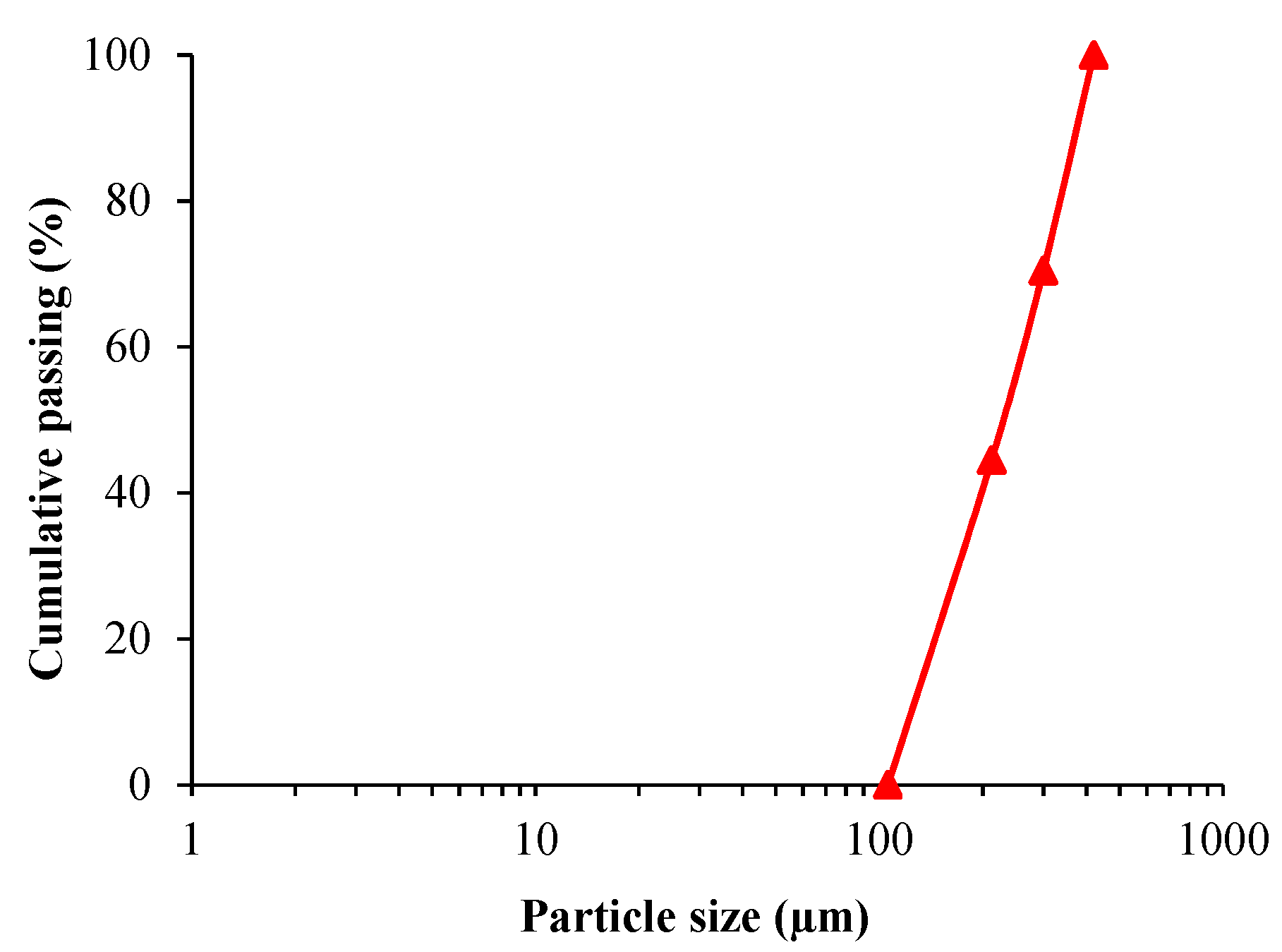
2.1. Quartz Sample and Flotation Reagents

Pure quartz samples (99.9%, −425 + 106 μm) were used for the flotation experiments in this work. The chemical composition of the quartz sample was identified using an X-ray fluorescence spectrometer (XRF, PW 2404 model, Philips, Amsterdam, The Netherlands) as listed in

Table 2. Chemical composition of the quartz sample.

Component	SiO2	Al2O3	CaO	Na2O	Fe2O3	K2O	MgO	P2O5	SO3	L.O.I *
Content (wt%)	99.901	0.011	0.010	0.007	0.010	0.007	0.004	0.005	0.008	0.037

* L.O.I: loss of ignition.

. Firstly, quartz samples were crushed using a laboratory jaw crusher with a maximum compression resistance of 300 MPa. The next step was to use a roll crusher (WEDAG, Cologne, Germany) to reduce the particle size to reach the range of −425 + 100 µm (finer than 425 µm and coarser than 100 µm), which is the typical particle size used for coarse quartz flotation. Following this, this fraction size was screened in a dry environment using the standard US sieve series and Tylermeshed sizes (50, 70, and 140 mesh). Flotation experiments were conducted with three different size classes (namely −425 + 300 µm, −300 + 212 µm, and −212 + 106 µm) (Figure 1).

Dodecyl amine (50 g/t, C₁₂H₂₇N) with a purity of 99% and Methyl Isobutyl Carbinol (22.4 ppm, MIBC, C₆H₁₄O) with a purity of 98% were used in the flotation experiments as the collector and frother, respectively. These surfactants were provided by Merck and Sigma-Aldrich Company (St. Louis, MO, USA).

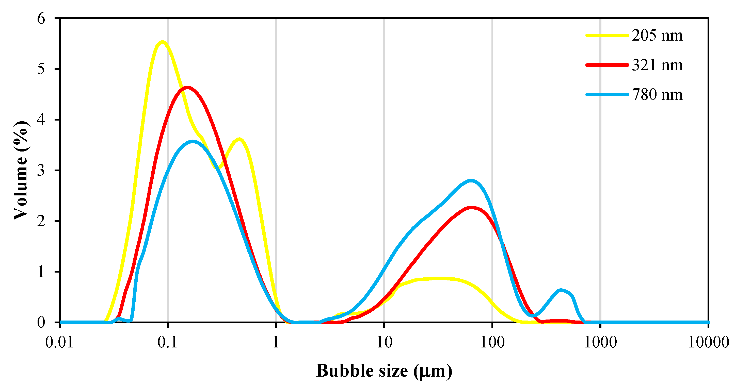
2.2. Operating Variables and Experimental Design

Effective operating variables and their levels were considered according to our previous results [47].

Table 3. Operating factors and their studied levels in the experimental design.

Factor	Name	Unit	Minimum	Maximum
A	Air flow rate	L/h	30	60
B	Impeller speed	rpm	600	1300
C	MNB diameter	μm	0	293
D	Particle size	μm	106	600
Response	Recovery	%	9.98	95.59

lists the operating factors and their experimental levels used in the experimental design. The effects and interactions of each operating parameter were evaluated using a historical data (HD) experimental design with 192 experimental runs. The HD method is an effective technique in the analysis of experimental design with a large number of test runs. The HD design is a subset of response surface methodology with a flexible structure so that the engineer can use any favorable design with unlimited numbers of input variables and runs. In this method, there is no need to predefine the absolute values for any variable’s level. Actually, the HD design employs the minimum and maximum values for every individual variable observed during experimental investigations. Then, software can perform the statistical analysis based on the responses measured for every set of conditions that randomly appears in the DOE. Moreover, it can give deep knowledge about the nonlinearity of effects as well as potential interactions among operating variables [42]. In the present study, we assessed the quartz recovery (%) as a process response. The experimental results of the HD design are presented in Supplementary Data.

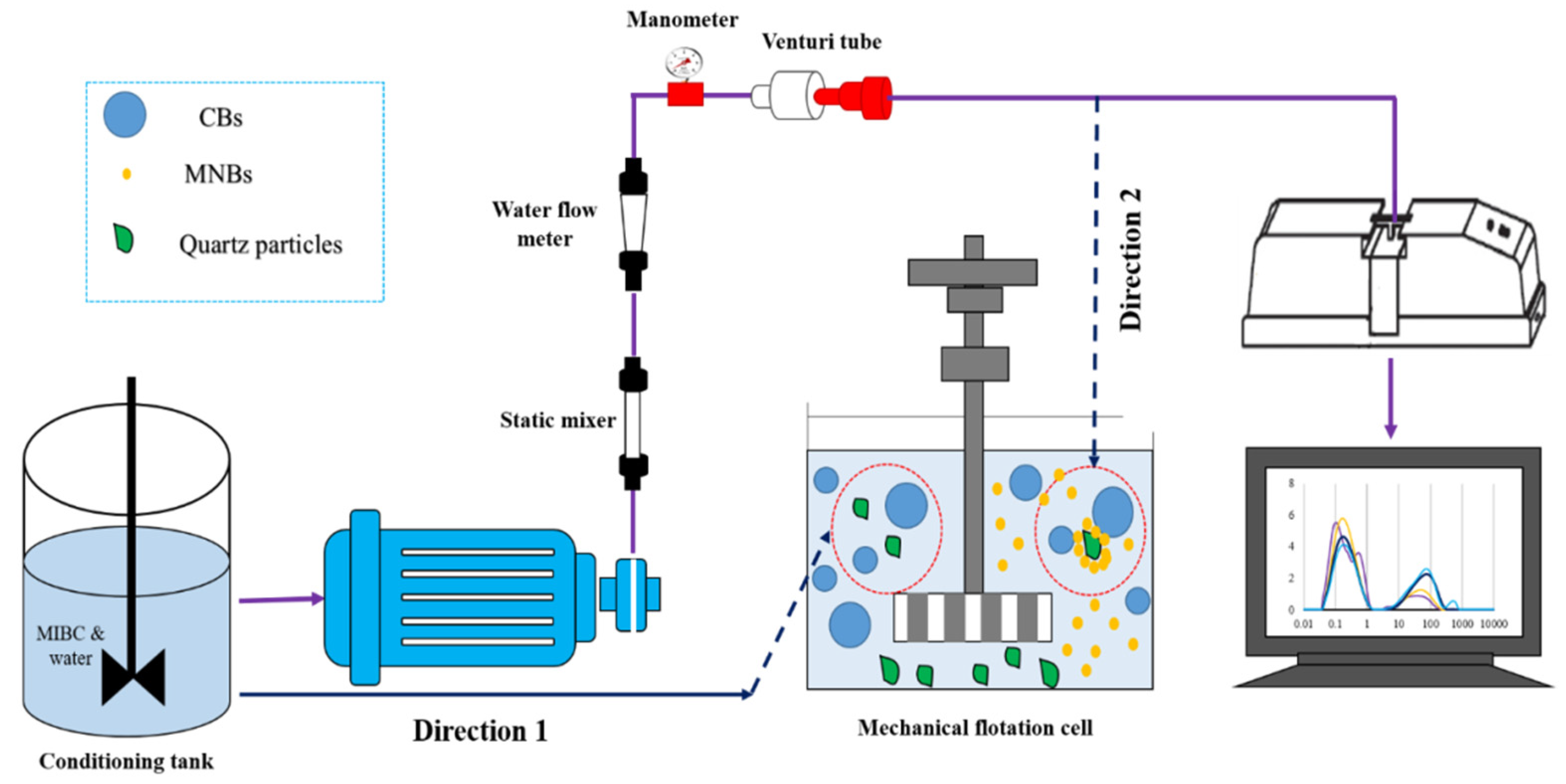
2.3. Flotation Experiments and Calculations

Flotation experiments were carried out in a 1 L mechanical flotation cell. For each experiment, 140 g of coarse quartz particles was added to tap water (with a pH of 7.0 ± 1) to prepare the required pulp with a given solid content. The air flow rate was set at 30 and/or 60 L.min⁻¹, and the flotation was implemented for 3 min at an impeller speed ranging between 600 and 1300 rpm (the sizes of the produced air bubbles in the system were measured to be 0.5–1 mm). Prior to the addition of the flotation reagents, the quartz pulp was mixed for 1 min. The perquisite amount of collector was then added to the pulp followed by 2 min of conditioning. Next, a given dosage of the frother was added to the flotation cell through the following modes (Figure 2):

• In the absence of MNBs, the solution of the frother was directly added to the system through direction (1).
• In the presence of MNBs, 23 wt.% of the frother was first directed to the cell via direction (1), and after 30 s, the rest of frother mass was injected through the direction (2).

Finally, the air inlet valve was opened to form the froth. The froth phase formed over the pulp zone was steadily collected for 2.5 min. After each experiment, the floated and tailing samples were dewatered and weighted to calculate the flotation recovery of quartz particles. Detailed information regarding the chemical reagents and operating parameters is given elsewhere [4]. All flotation experiments were performed at ambient temperature (25 ± 1 °C).

The bulk MNBs were prepared using 22.4 mg/L of MIBC at the natural pH of 7.0. The prepared solution was pumped through a centrifugal pump (PM80, Pentax, Veronella (VR), Italy) into a Venturi tube with specific dimensions (as a cavitation device). An air flow rate of 24 L/h was employed to inject filtered air into the solution. To increase the solubility of air, two static mixers were used, as shown in Figure 2. As a result, they were installed both downstream and upstream of the pump. Air’s solubility increased at the Venturi tube’s entrance, leading to a high static pressure (0.35 kPa). Depressurization of the air-saturated solution caused bulk NBs to be produced when it reached the Venturi tube. The bubble size distribution was measured using a laser particle size analyzer (LPSA). Detailed experimental setups are presented in the previous studies [4,7]. Bubble sizes were measured using a laser particle size analyzer (LPSA, model 2000 MS, Malvern, UK). Figure 3 exhibits the bubble size distribution (BSD) of generated MNBs. As seen, there are two main picks related to the microbubbles (10–100 µm) and nanobubbles (0.01–1 µm). It is worth noting that bubbles finer than 1 µm are counted as nanobubbles (also known as ultrafine bubbles) as discussed in detail in our previous studies [6].

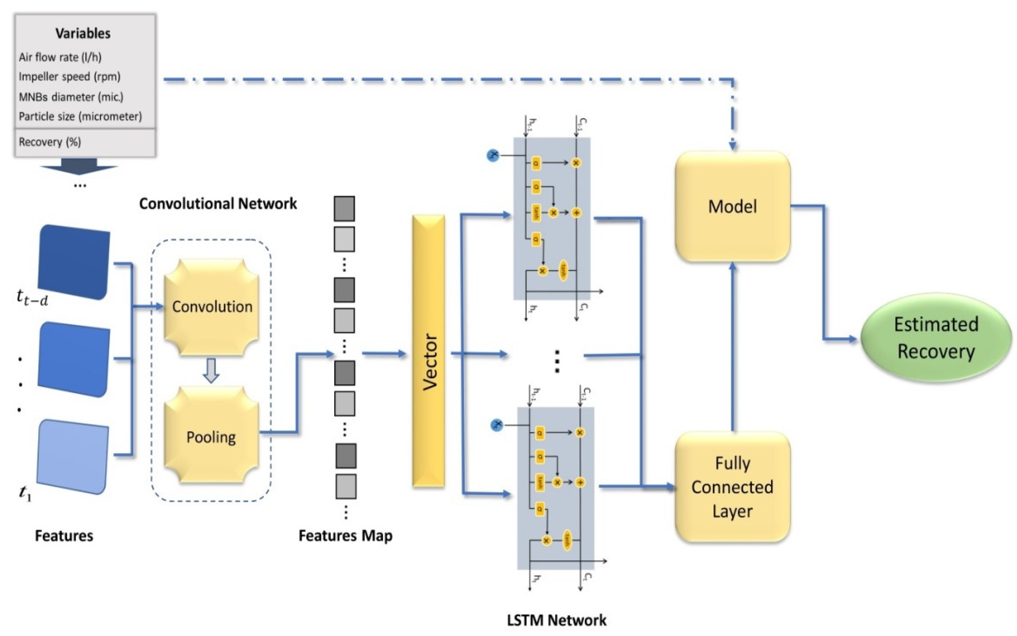
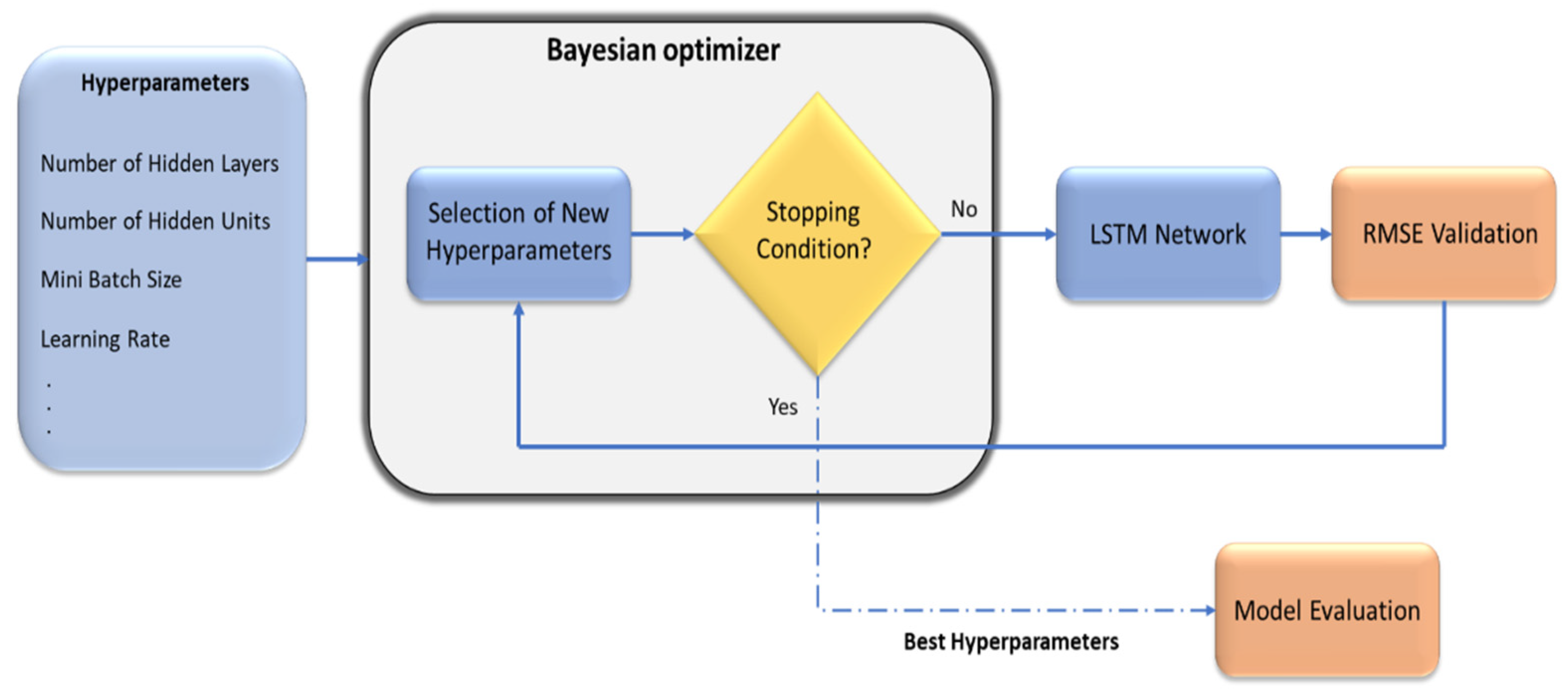
2.4. Deep Learning Simulation

This work employed a hybrid CNN-RNN model to build a predictive model for quartz recovery estimation. There are usually several convolutional and pooling layers in convolutional neural networks (CNNs), followed by a few fully connected (FC) layers. A CNN is designed with several parameters, such as the number of kernels, kernel size, padding type, and stride. Kernels are matrices of weights to convolve with the input volume and are used to extract features. The padding preserves the size of the feature maps by adding zeroes to the input; otherwise, they can shrink in each layer. Stride is a kernel’s parameter that modifies the amount of movement over the data. Recurrent neural networks (RNNs) are also applicable in modeling sequence data [48]. An RNN does indeed capture time variations and makes favorable predictions over a conventional neural network that incorporates feed-forward neural networks [49]. RNNs have hidden units called state vectors, which act as an internal memory and are capable of retaining information over time. Although RNNs are powerful for sequence data, their training is challenging because of vanishing and exploding gradient problems [50]. It was Hochreiter and Schmidhuber who introduced the first LSTM network to address the problem of vanishing gradients [51]. A number of sequence modeling applications have demonstrated the superiority of LSTM networks over other time series models because they do not require the specification of the nonlinear functions to be estimated [52,53].

This paper leverages CNN specifications and the LSTM algorithm for extracting valuable information from input data and handling time series problems. The LSTM input is the CNN output. The diagram of the proposed model is shown in Figure 4. Air flow rate, impeller speed, MNB diameter, and particle size are included in the prediction model, as the output is quartz recovery.

To express the deep learning model for quartz recovery using MNBs, x_i is the input data, y_i is the output data before decoding using a fully connected layer, Ω is number of layers, and µ is the current trained layer. Convolutional, pooling, and LSTM layers also produce $C{l}_i^{\mu }$, $P{l}_i^{\mu }$, and $L{l}_i^{\mu }$ as outputs, respectively. The developed deep learning model can be described as follows:

$$\begin{array}{l}C{l}_i^u=g\left(u^T{x}_i\right)\mu =2\\ P{l}_i^u=g\left({\upsilon }^{T}C{l}_i\right)2<\mu <\delta -3\\ L{l}_i^u=g\left(w^T{P}_i+d^T{L}_i\right)3<\mu <\delta -2\\ y_i^u=f\left({\xi }^T{L}_i\right)\mu =\delta -2\end{array}$$

(1)

In these equations, the prediction model’s weight matrices are u, v, w, d, and ξ. Eventually, y_i is decoded by the fully connected layer, and the recovery rate as the final result is obtained.

2.5. Modeling Process

Processing the input data in order to extract features and correlations is important. Afterwards, time series features need to be extracted. A CNN can combine features of neighboring regions using convolution kernels in order to achieve ‘features’ spatial correlations [54]. Therefore, extracting data features before training the CNN is unnecessary because it can learn these features automatically from input data. Generally, it is effective to generate multiple convolved features from the input data by applying different convolution kernels, which are typically more useful than the original features of the input data. Data are entered as a two-dimensional tensor. The main core of the CNN is the convolution layer, which accounts for the majority of convolutional neural network calculations. Each convolution layer in the convolution neural network includes a set of filters, and the input layer is convoluted with a set of filters to derive the output. The outcome of the convolution layer is a feature map. The convolutional filters move over the input tensor and scan it to extract meaningful patterns. Actually, a convolutional layer produces new feature values by applying convolution operations between raw input data and convolution filters [55]. As with other neural networks, convolutional neural networks employ a nonlinear activation function after the convolutional layer. An activation function is used to generate the output feature map. The convolutional kernel of the new layer studies the output feature maps of the previous layer and, using the activation function, its feature maps are generated. When the feature map is convoluted in a CNN, N feature maps are input to the pooling layer, producing N features of contractible size.

As part of a convolutional neural network, the pooling layer also plays an important role. With the pooling layer, the spatial size of the feature map obtained through the convolution layer can be reduced. The pooling layer works like convolution and moves over the input tensor. A back-propagation algorithm was used to train the CNN. The training accuracy of CNN training was measured using MSE. Convolution layer weights are updated according to training accuracy during the training and optimization process. Having determined the actual data features and compressed the two-dimensional input matrix, the final estimation model was trained. Input to the LSTM layer came from the CNN’s last pooling layer.

One of the important points in using deep learning methods is to choose appropriate values for the hyperparameters. Our final predictive model parameters do not minimize the loss function if we do not properly tune our hyperparameters. Thus, our model makes more errors. In this work, a Bayesian optimizer was used for tuning hyperparameters of the predictive model to achieve the best results. Figure 5 shows the path of hyperparameter tuning using the Bayesian optimizer.

Table 4. CNN-LSTM model parameters.

No.	Parameter	Value	No.	Parameter	Value
1	Training method	Stochastic gradient descent	6	Number of LSTM layers	1
2	Kernel size of convolution layer	7 × 7	7	Number of LSTM nodes	200
3	Kernel size of pooling layer	3 × 3	8	Number of fully connected layers	2
4	Number of convolution layers	1	9	Learning rate	0.001
5	Number of pooling layers	1	10	Batch size	50

shows the parameter values of the CNN-LSTM model.

For comparison purposes and to provide a better understanding of the performance of the CNN-LSTM model, the following prediction models were also investigated:

• The radial basis functions neural network (RBFNN) is a special type of artificial neural network that measures the similarity between data based on distance, and the technique is considered an effective method for interpolating in multidimensional spaces [56]. It is a feed-forward neural network, which, like many other artificial neural networks, consists of inputs and hidden and output layers. Trial and error led to RBFNN’s proper structure being 4-9-4-1. There was an overfitting effect when there were more neurons.
• The gated recurrent unit (GRU) was introduced to reduce LSTM overload and to address the limitations of traditional RNNs. This algorithm is generally considered a simpler and modified version of LSTM because both methods utilize the same design. Unlike LSTM, it has one fewer gate, which can reduce matrix multiplication and speed up computation. This algorithm’s parameters were also adjusted to obtain suitable results for comparison. The number of epochs, which means one complete pass of the training dataset through the algorithm, was set to 1000, a learning rate of 0.001 was the step size at each iteration, and three hidden layers and Adam optimizer were used for the training process.

2.6. Correlation and Feature Importance

Pearson correlation coefficients (PCCs): Generally, a correlation coefficient is a way of predicting the value of one variable by evaluating its relationship to another. To measure how two quantitative variables are related, one of the most popular methods is to use Pearson correlation coefficients. The formula is presented as follows:

$$corr\left(X,Y\right)=\frac{E[(X-E(X))(Y-E(Y))]}{{[V(X)V(Y)]}^{\frac{1}{2}}}$$

(2)

where E and V are the mathematical expected value and variance, respectively.

Shapley additive explanations (SHAP): SHAP was used to measure the feature importance in the final model. It is a machine learning approach for explaining a model’s predictions and providing interpretability of a model [57]. Overall, when each variable might have contributed more or less than the others, the Shapley value helps to determine a payoff for all of the variables [58]. The Shapley value (ϕ) for a model (f) can be calculated as below:

$${\varphi }_i(f,x)={\displaystyle \sum _{S\subset M\backslash i}\frac{\left|S\right|!(|M|-|S|-1)!}{\left|M\right|!}}\left[f(S\cup \{i\})-f(S)\right]$$

(3)

where M is the input variables, S is a subset of M with the ith feature excluded from M, and f (S ∪{i}) − f (S) is the marginal feature contribution of the ith variable [59,60].

3. Results and Discussions

3.1. Historical Data Model Development and Analysis

In this study, Design Expert v.7.0 software (Stat-Ease Inc., Minneapolis, MN, USA) was used to model experimental data. The stepwise procedure regarding the application of Design Expert software is explained in detail elsewhere [61,62]. Based on our efforts, the most accurate quadratic model for quartz recovery was obtained as follows:

$$Recovery=67.31-2.69A-8.23B+4.45C-25.13D-0.83AD-2.48BC-18.62B^2-12.12C^2+2.15D^2$$

(4)

where factors are in coded form. The results of the reliability analysis for estimating the model coefficients are given in Appendix A (

Table A1. Reliability analysis results for model coefficient estimation.

Factor	Coefficient Estimate	df	Standard Error	Low 95% CI	High 95% CI
Intercept	67.31193	1	0.806602	65.72038	68.90348
A	−2.68694	1	0.32382	−3.32589	−2.04799
C	−8.22807	1	0.510746	−9.23585	−7.22028
D	4.454524	1	0.451484	3.563676	5.345372
E	−25.1352	1	0.395191	−25.9149	−24.3554
AD	−0.8273	1	0.394632	−1.60597	−0.04863
BC	−2.47679	1	0.683466	−3.82538	−1.1282
B2	−18.6229	1	0.868306	−20.3362	−16.9096
C2	−12.1164	1	0.746886	−13.5902	−10.6427
D2	2.145962	1	0.695365	0.773897	3.518026

). As seen, all coefficients sit within the lower and upper reliability limits based on a 95% confidence interval (CI). The validation parameters for the developed models revealed that the suggested prediction model is significant due to its high value on Fisher’s F-test (578.19) and low probability value (p model < 0.0001). Another piece of evidence for the significance of the proposed model Equation (4) is a uniform normality plot for flotation recovery, as shown in Figure 6, approving the assumptions of normal probability and independency during the statistical analyses [63]. Moreover, the significant values of accuracy measures of the model, i.e., the normal correlation coefficient (96.64%) and adjusted correlation coefficient (96.47%), designate the reliability of the developed model. The prediction reliability of the model can be confirmed based on its high predictive correlation coefficient of 96.25% [63]. This is also evident from the plot illustrating the predicted values versus experimental data in Figure 6. Another statistical measure showing the accuracy of the model equation is the ratio of signal to noise called adequate precision. For the quartz recovery model, the adequate precision of 93.99 is significantly greater than the minimum desirable value of 4 [64] and implies that the models can navigate the design space with high reliability.

Therefore, the model Equation (1) was used to analyze the significance of the effect of operating factors on quartz recovery using the analysis of variance (ANOVA) method within a confidence interval of 95%. Appendix A (

Table A2. Analysis of variance results for flotation response of quartz recovery.

Source	Sum of Squares	df	Mean Square	F Value	p-Value
Model	104,025.7	9	11,558.41	578.1945	<0.0001
A-Air flow rate (L/h)	1376.361	1	1376.361	68.85069	<0.0001
B-Impeller speed (rpm)	5188.111	1	5188.111	259.5286	<0.0001
C-MNBs (nm)	1945.999	1	1945.999	97.34608	<0.0001
D-Particle size (μm)	80,867.34	1	80,867.34	4045.285	<0.0001
AD	87.85426	1	87.85426	4.394797	0.0374
BC	262.523	1	262.523	13.13238	0.0004
B2	9195.465	1	9195.465	459.9914	<0.0001
C2	5260.96	1	5260.96	263.1728	<0.0001
D2	190.3892	1	190.3892	9.523975	0.0023
Residual	3618.284	181	19.99052
Cor Total	107,643.9	190

) shows the ANOVA results and implies that the effects of all factors are statistically significant due to their p-values being less than 0.05. Moreover, the only significant interaction effects are those between air flow rate and particle size (AD) and impeller speed and MNB size (BC).

3.2. Interpretation of Main and Interaction Effects

Figure 7 shows the main effect plots for operating factors considered in the experimental design. Detailed explanations regarding the construction of main effect plots are addressed elsewhere [34,65,66,67]. According to Figure 7, quartz recovery decreases as the air flow rate increases. There is an optimal air flow rate in every flotation system over which the flotation rate decreases due to undesirably increased turbulence in the pulp zone. Such a turbulent regime can interrupt the efficient attachment of particles to bubbles in both pulp and froth zones and cause bubbles to release their loads [68]. The impeller speed imposed a nonlinear effect on quartz recovery such that maximum recovery can be reached at a speed of about 850 rpm, after which the recovery significantly drops from about 67% down to 40%. Generally, as the impeller speed increases, the improved dispersion of both bubbles and particles in the pulp zone may lead to enhanced particle–bubble collision and, consequently, improved recovery of quartz particles. However, over the optimal impeller speed, the turbulent regime increases such that the loaded particles are forced to release their carried particles back to the pulp. This, in turn, results in the sharp decrease in recovery observed in Figure 7. As the diameter of MNBs increases, the rate of quartz recovery to the concentrate improves significantly. Larger bubbles have higher rise velocity and thus increase the chance of particle-to-bubble attachment [69,70]. The size of zero for MNBs represents the system without MNB injection. Regardless of the increasing relationship between the quartz recovery and the size of MNBs, the presence of MNBs itself has a positive effect on the performance of the flotation system compared to the process without MNB injection. Decreasing the recovery of coarse particles could be due to low particle–bubble stability while being lifted to the froth zone. Additionally, a reduction in the recovery of large bubbles can be related to a decrease in lower interceptional collision probability because particles tend to follow streamlines at a distance away from the bubble [70]. As the size of quartz particles increases from 106 to 300 μm, the recovery is expected to drop dramatically most likely because of the decreased carrying ability of bubbles. One possible reason for not observing the optimum level of recovery versus particle size can be the selected particle range in this study.

The interaction between two operating factors can be effectively evaluated using 3D response surface plots. These plots are constructed using mean values of the process response calculated using a model equation (Equation (4)) versus those two factors with a significant interaction as indicated by ANOVA (Table A2). Similar to main effect plots, the other factors are maintained at their mid-levels during the development of the interaction surface plots [29]. Figure 8 shows the 3D response surface plots for significant interactions given in Table A2 (Appendix A), i.e., interactions between air flow rate and particle size (AD) and impeller speed and MNB size (BC). As seen in Figure 8, the interactive behavior of the variables completely corresponds to their individual effects. In the case of AD effect, for example, maximum recovery may be obtained when both air flow rate and particle size are at their low levels. Similar to the conclusion that emerged from main effect plots, recovery culminates at values around the middle level of impeller speed and MNB size. These interactive results confirm the reliability of those results observed from individual effect plots.

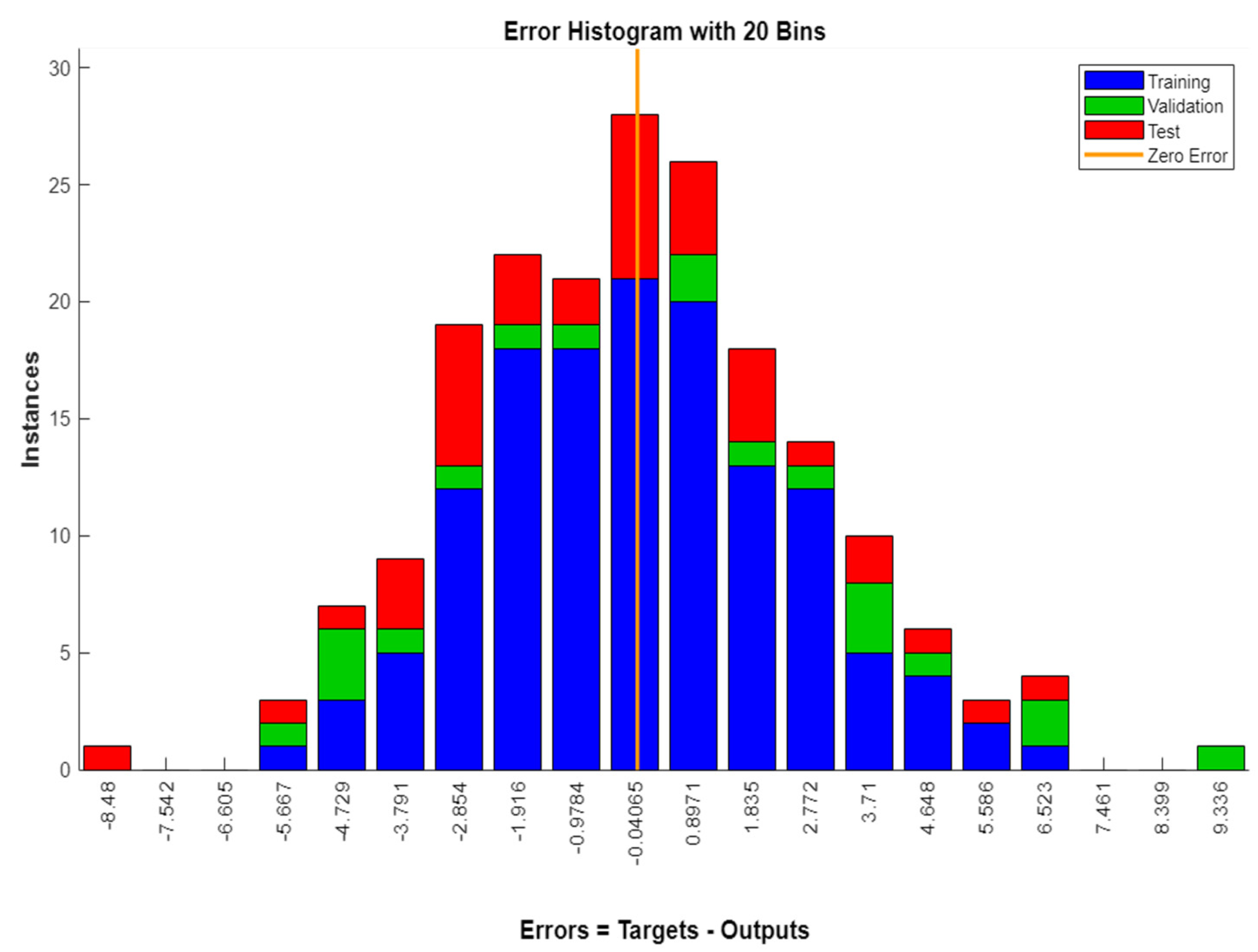
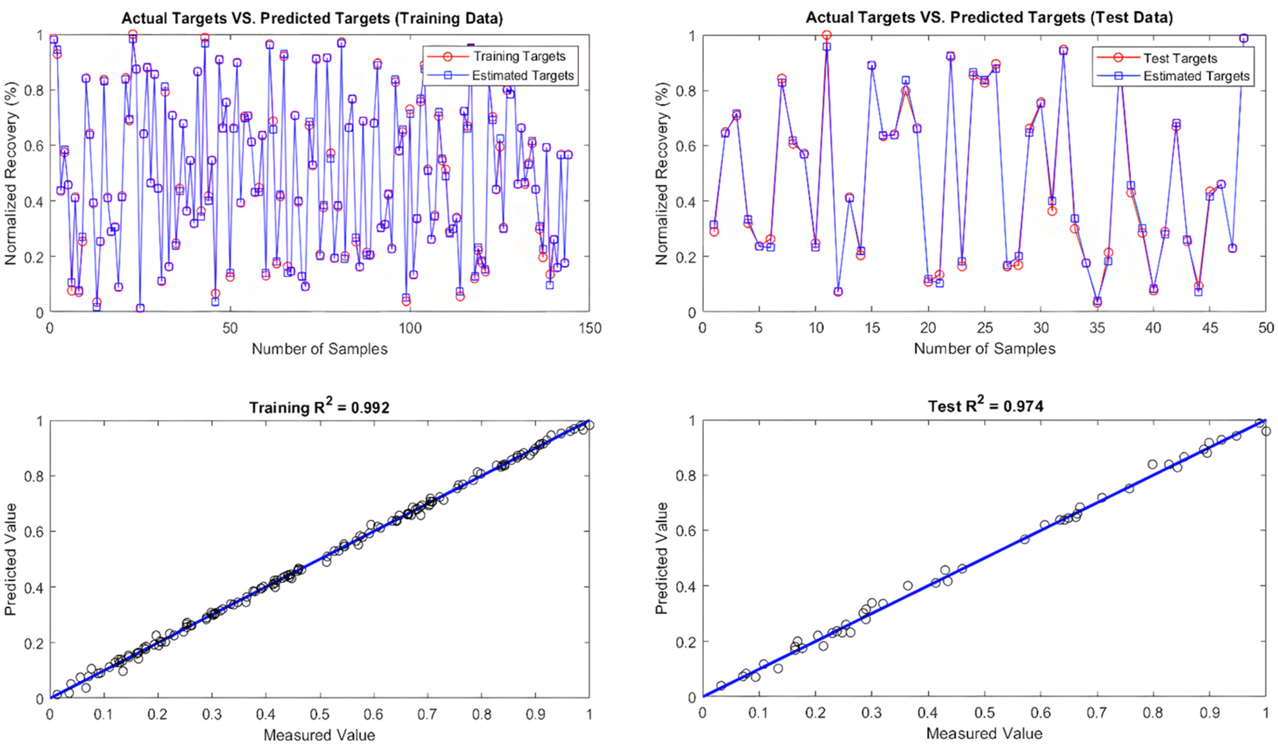
3.3. Deep Learning Simulation Results

All three modeling algorithms were implemented efficiently to estimate quartz recovery. In the modeling process, ten percent of the data were used as validation data in the training stage to prevent overfitting and hyperparameter tuning. A total of 70% and 20% of the data were used for training and testing the models, respectively. To evaluate the models after the testing process, the following equations were used:

$$RMSE=\sqrt{\frac{1}{n}{{\displaystyle \sum }}_{i=1}^n{\left(y_i-{\widehat{y}}_i\right)}^2}$$

(5)

$$R^2={\left(\frac{{{\displaystyle \sum }}_{i=1}^N\left(y_i-\overline{a}\right)\left({\widehat{y}}_i-\overline{e}\right)}{\sqrt{{{\displaystyle \sum }}_{i=1}^N{\left(y_i-\overline{a}\right)}^2}\sqrt{{{\displaystyle \sum }}_{i=1}^N{\left({\widehat{y}}_i-\overline{e}\right)}^2}}\right)}^2$$

(6)

Based on the RMSE and correlation of determination for quartz recovery,

Table 5. Evaluating results for the estimation of quartz recovery.

Model	Training RMSE	Training R2	Testing RMSE	Testing R2
CNN-LSTM	0.0096	0.992	0.045	0.974
RBF	0.228	0.886	0.252	0.873
GRU	0.097	0.935	0.182	0.909

compares the performances of the three models on both training and testing datasets.

In contrast to the other two models, the hybrid CNN-LSTM model performed significantly better. To extract spatial features of quartz recovery, a CNN was used as a basis for the model. The input time series features were then extracted using an LSTM. This method has the advantage of eliminating redundant data through CNN processing and obtaining actual features from the data. As an added benefit, the prediction model was simplified as CNN uses shared weights. LSTM also captured the internal dependencies and considered data nonlinearity. Because of having advantages of both CNN and RNN methods, it can be concluded that the proposed structure is suitable for processing large datasets from mining sites and processing plants. In the following, Figure 9 demonstrates the error histogram of CNN-LSTM, and an illustration of the CNN-LSTM model’s fitting and regression diagrams can be seen in Figure 10.

An error histogram is a representation of how a neural network performs after being trained and compared with the target values. Error value is defined as the difference between predicted and target values; hence, these can be negative. In Figure 9, vertical bars are presented as bins. There are 20 bins in this histogram, which represent the total error range. The Y-axis represents the number of samples falling within a particular bin. An example is the bin at the center of the histogram corresponding to the error value of −0.04065 whose heights for training and test datasets lie at about 20 and near 30, respectively. This indicates that many samples had an error of around −0.04065.

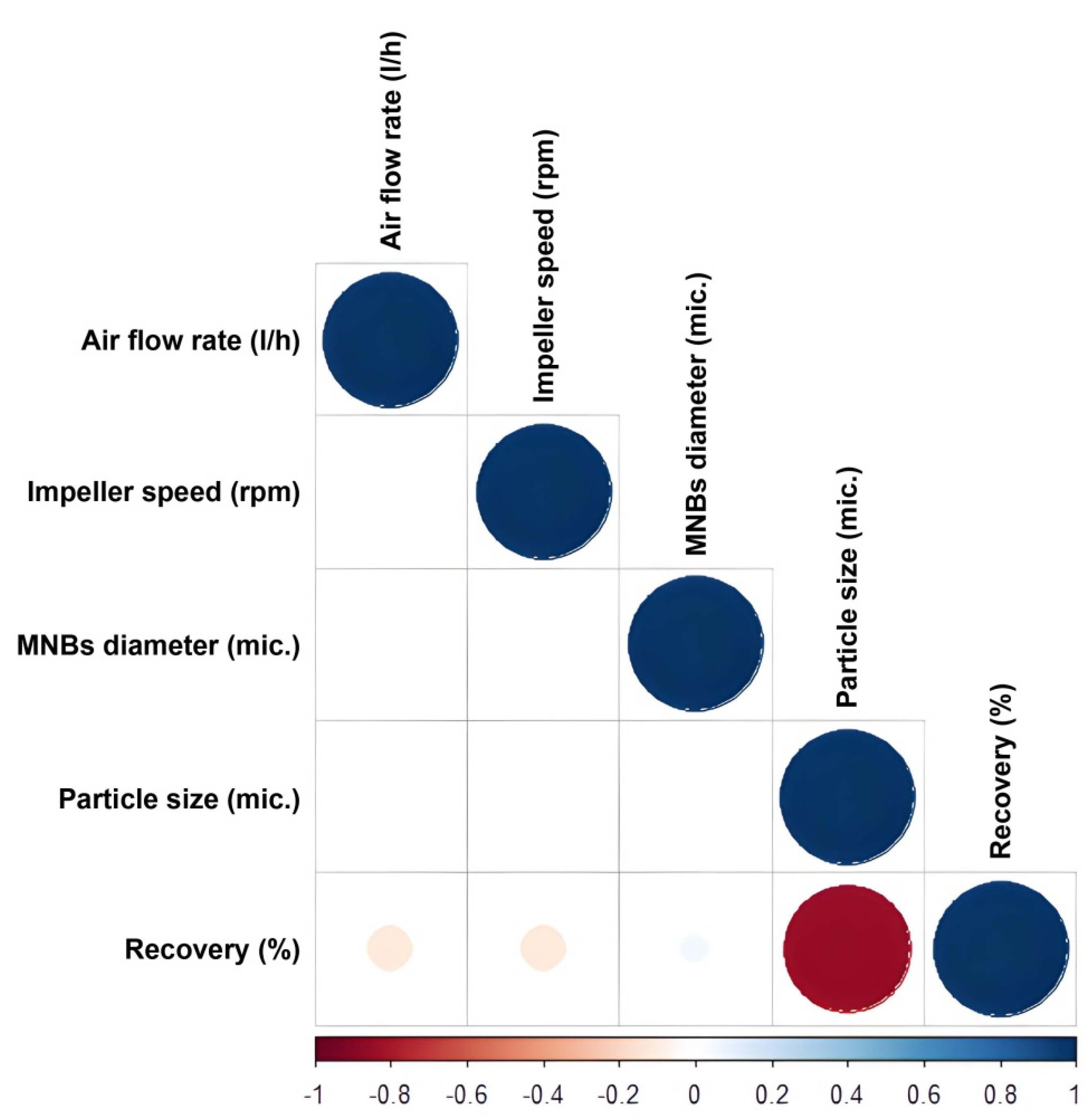
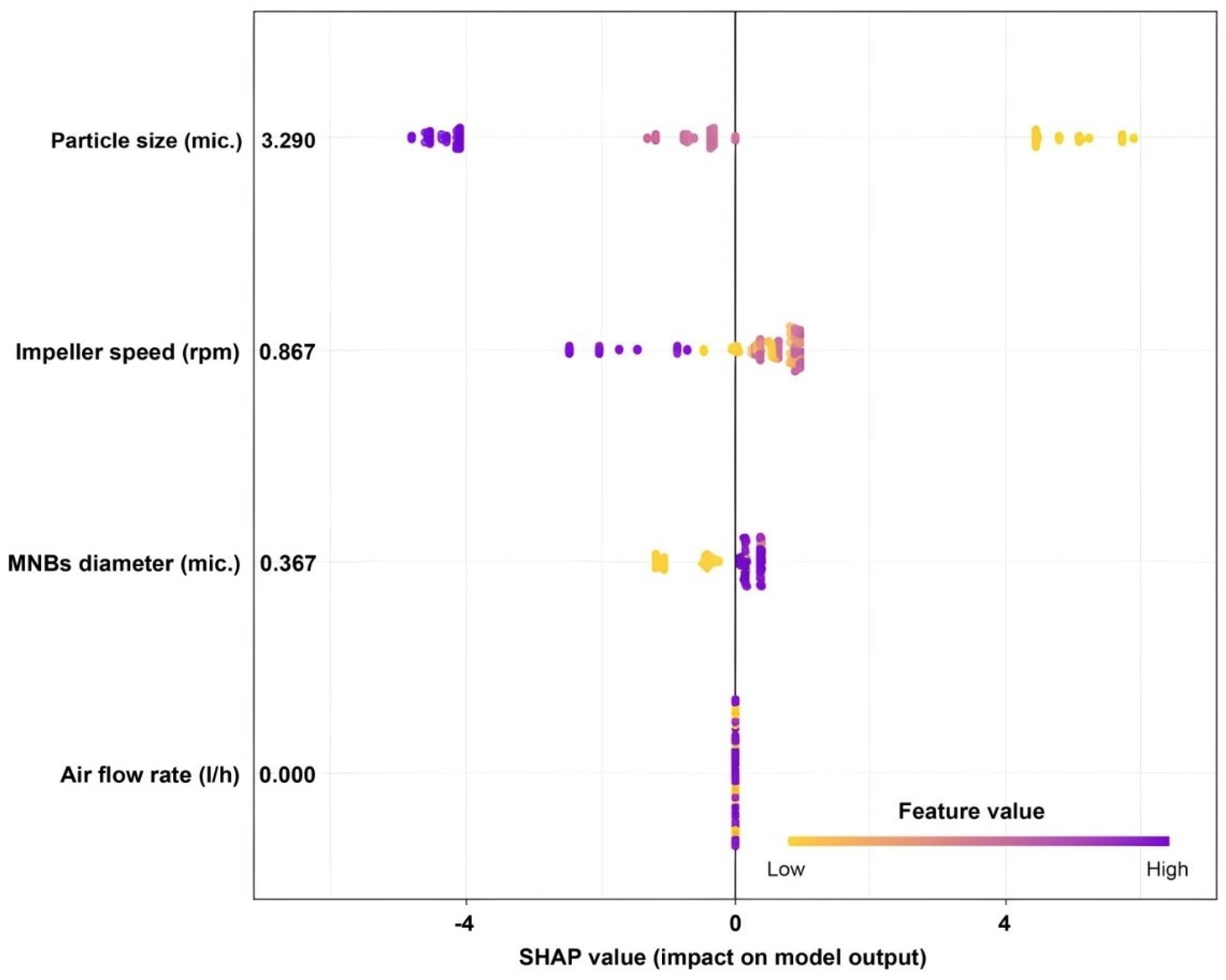
3.4. Correlation and Feature Importance Results

To estimate the relationships between the variables, the Pearson coefficient was also calculated, the results of which can be seen in Figure 11. In general, there is a linear relationship between the two variables when the correlation coefficient is close to 1 or −1.

There is a challenge to understanding the blackbox property of deep learning methods, including CNN-LSTM, and further research is required. In order to check how these models work, feature importance methods were developed. The SHAP method is used in this paper, and the general working method of SHAP is briefly explained below. The term “neural network” refers to a network of artificial neurons connected together, and they can transmit signals between the neurons. Each neuron’s output is calculated by a nonlinear function of the sum of its inputs, which is a real number of connections. In SHAP analysis, different input features are scored according to how relevant they are for the trained model based on comparisons of neuron activation. In other words, feature importance is calculated using SHAP analysis by considering the marginal contribution of each feature to the model outcome. The SHAP analysis was performed using the entire dataset. Figure 12 shows the SHAP values for the CNN-LSTM prediction model. SHAP computed SHAP values based on the contributions of each sample.

SHAP (Figure 12) ranked variables based on their importance and illustrated that particle size, impeller speed, and MNB diameter had the highest impact on the output, in order. In this regard, PCC showed that particle size had a strong linear relationship with the recovery. The smaller the particle size, the greater the recovery. SHAP could model relationships much more accurately than Pearson correlations, even though there is good agreement between the two methods. Using Pearson correlations, only linear relationships can be examined, and their magnitudes can be determined, while SHAP assesses the multivariable relationships by identifying their linear and nonlinear interactions, evaluating their importance, and highlighting their magnitude. For instance, in contrast to linear analysis by Pearson correlation that found no significant interactions between impeller speed or MNB diameter and quartz recovery, SHAP showed that there are influential variables. The induction time between large bubbles and particles within flotation machines tends to be shorter when nanobubbles are present, which increases contact angles [71]. Consequently, MNBs can improve particle collection efficiency and increase flotation velocity [72]. Another important parameter in flotation is impeller speed, which must be adjusted optimally to avoid reducing system efficiency. Using values lower than their optimum value, for example, will prevent the dispersion of particles within the flotation cell and result in fewer collisions. An excessive amount also causes turbulence in the collection and even the froth zone, reducing the efficiency of the particle–bubble attachment. According to [73], stirring speed plays a key role in achieving optimal flotation, which is also related to flotation time.

4. Conclusions

In this study, an advanced simulation by hybrid serving of historical data (HD) and deep learning (DL) methods is presented and evaluated as a comprehensive approach to developing predictive models for quartz recovery estimation in the presence of MNBs at a laboratory scale. The following conclusions were obtained:

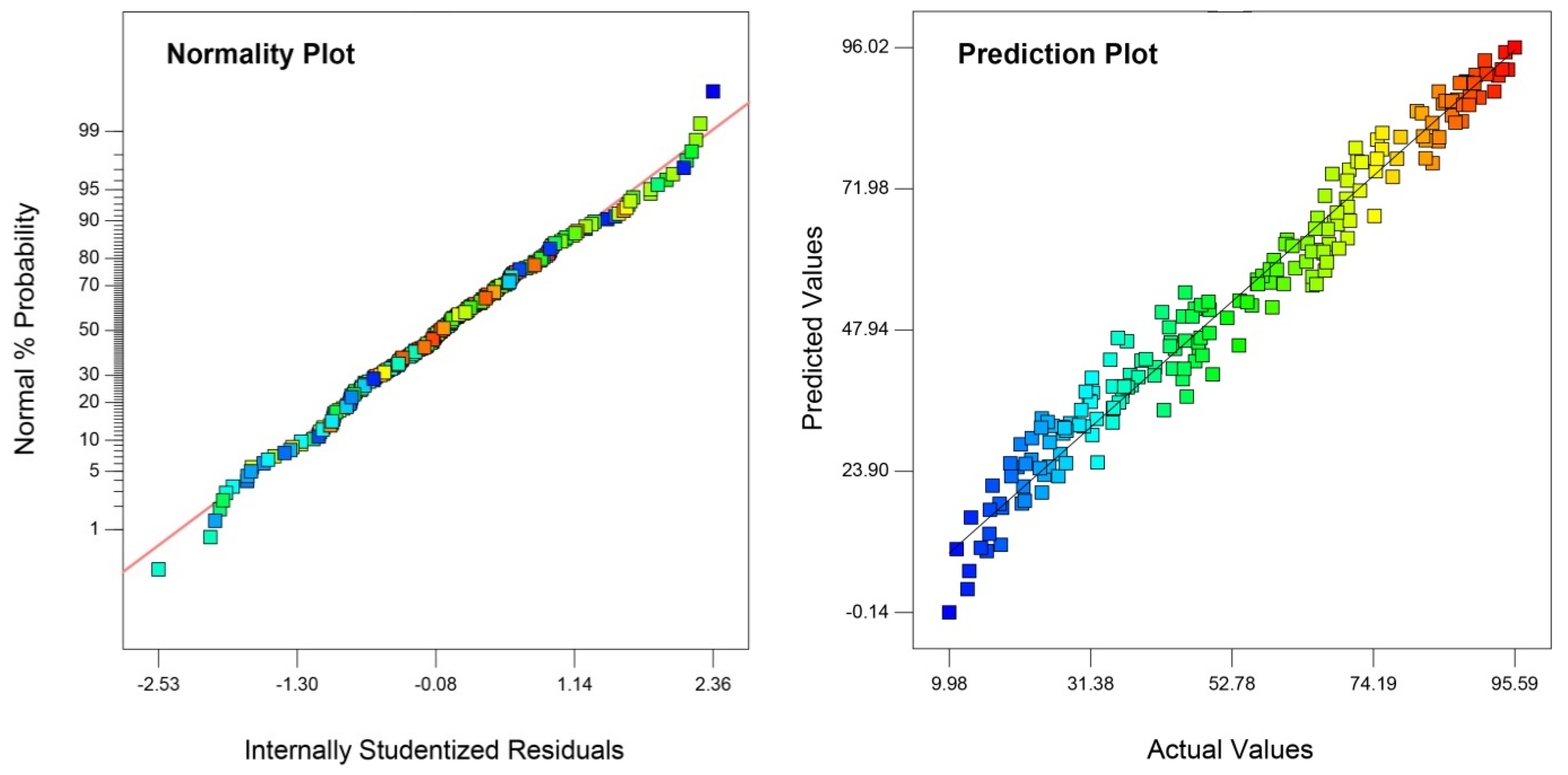
• The results of ANOVA within a confidence interval of 95% confirmed that all operational variables had statistically significant effects on process responses, and the proposed model was significant because of its Fisher’s F-test value (578.19) and low p-value (p model < 0.0001).
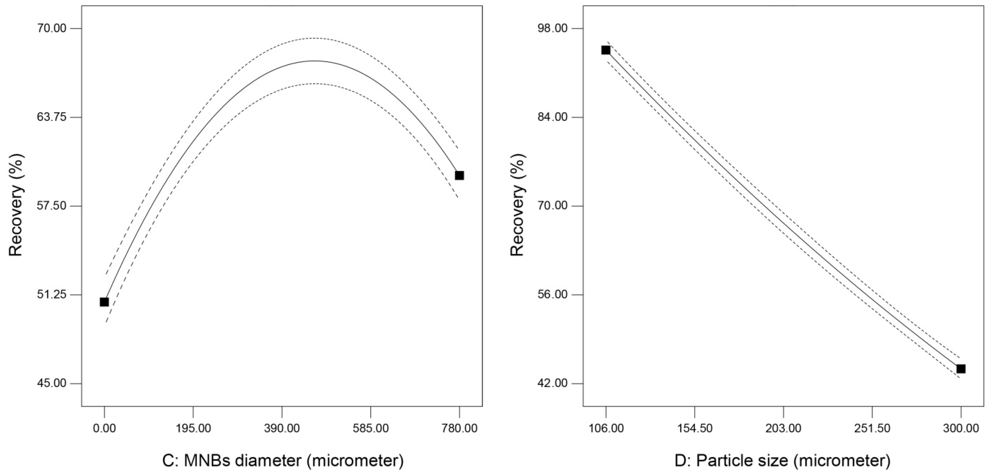
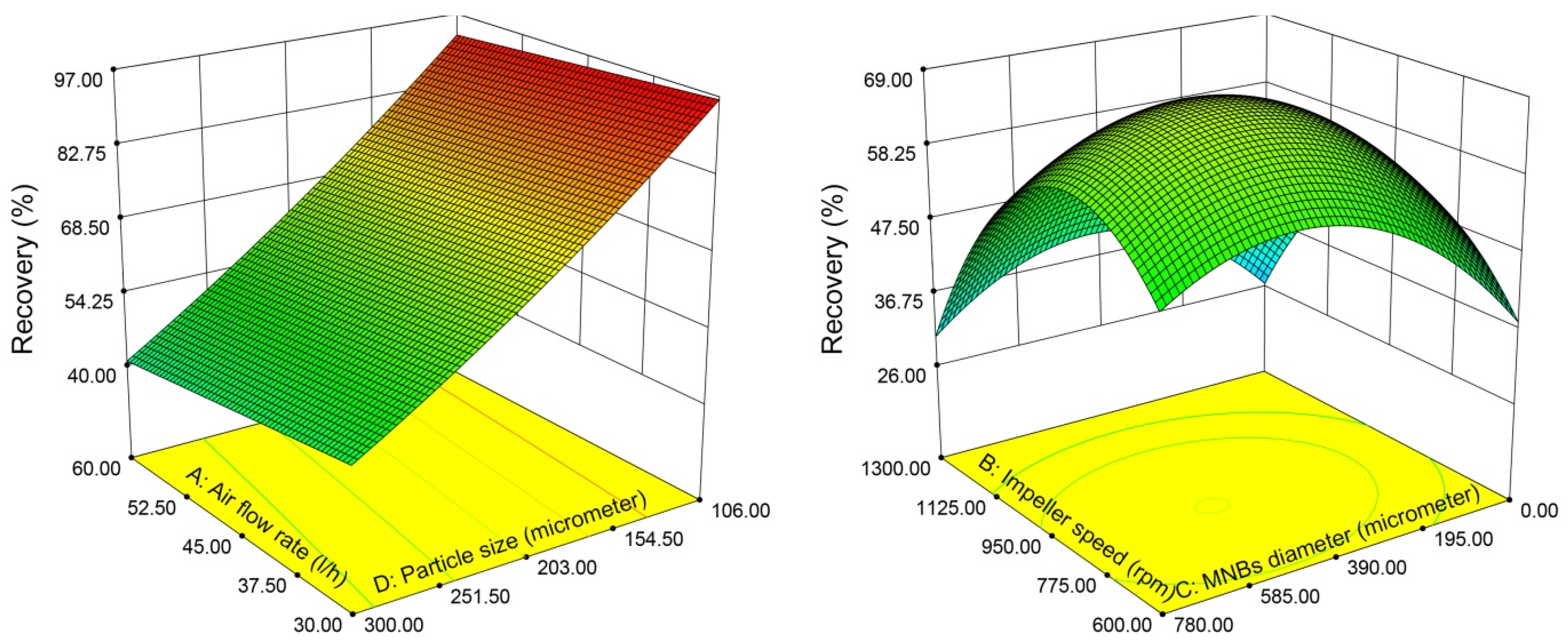
• A nonlinear effect of impeller speed was observed on quartz recovery when the speed reached 850 rpm, after which recovery dropped from 67% to 40%. Furthermore, as the air flow rate increased, quartz recovery was reduced.
• The blackbox property of deep learning models was identified as one of their principal limitations. The SHAP method was used for feature selection from the trained CNN-RNN model for it to be less of a blackbox and more understandable. Applying SHAP indicated that the particle size, impeller speed, and MNB diameter were ranked based on importance and shown to have the greatest impact on the metallurgical output. According to the PCC, particle size was strongly correlated with recovery. Additionally, recovery increased with decreasing particle size.
• Results showed that the SHAP and Pearson have a good correlation, but SHAP showed the potential to model relationships more accurately. Based on the Pearson correlations, impeller speed and MNB diameter did not interact significantly with quartz recovery, but SHAP indicated that there were significant influences.
• Based on the comparison of the results, it was concluded that the proposed CNN-LSTM hybrid model can be considered a reliable forecasting tool. This makes it a powerful tool for analyzing experimental data in other similar mineral processing processes.

References

1. Tao, D. Role of Bubble Size in Flotation of Coarse and Fine Particles—A Review. Sep. Sci. Technol. 2005, 39, 741–760. [Google Scholar] [CrossRef]
2. Faramarzpour, A.; Samadzadeh Yazdi, M.R.; Mohammadi, B.; Chelgani, S.C. Calcite in froth flotation- A review. J. Mater. Res. Technol. 2022, 19, 1231–1241. [Google Scholar] [CrossRef]
3. Liu, L.; Hu, S.; Wu, C.; Liu, K.; Weng, L.; Zhou, W. Aggregates characterizations of the ultra-fine coal particles induced by nanobubbles. Fuel 2021, 297, 120765. [Google Scholar] [CrossRef]
4. Nazari, S.; Hassanzadeh, A. The effect of reagent type on generating bulk sub-micron (nano) bubbles and flotation kinetics of coarse-sized quartz particles. Powder Technol. 2020, 374, 160–171. [Google Scholar] [CrossRef]
5. Rodrigues, W.J.; Leal Filho, L.S.; Masini, E.A. Hydrodynamic dimensionless parameters and their influence on flotation performance of coarse particles. Miner. Eng. 2001, 14, 1047–1054. [Google Scholar] [CrossRef]
6. Nazari, S.; Hassanzadeh, A.; He, Y.; Khoshdast, H.; Kowalczuk, P.B. Recent Developments in Generation, Detection and Application of Nanobubbles in Flotation. Minerals 2022, 12, 462. [Google Scholar] [CrossRef]
7. Nazari, S.; Shafaei, S.Z.; Gharabaghi, M.; Ahmadi, R.; Shahbazi, B.; Fan, M. Effects of nanobubble and hydrodynamic parameters on coarse quartz flotation. Int. J. Min. Sci. Technol. 2019, 29, 289–295. [Google Scholar] [CrossRef]
8. Zhang, Z.; Ren, L.; Zhang, Y. Role of nanobubbles in the flotation of fine rutile particles. Miner. Eng. 2021, 172, 107140. [Google Scholar] [CrossRef]
9. Zhou, W.; Liu, K.; Wang, L.; Zhou, B.; Niu, J.; Ou, L. The role of bulk micro-nanobubbles in reagent desorption and potential implication in flotation separation of highly hydrophobized minerals. Ultrason. Sonochem. 2020, 64, 104996. [Google Scholar] [CrossRef]
10. Nazari, S.; Zhou, S.; Hassanzadeh, A.; Li, J.; He, Y.; Bu, X.; Kowalczuk, P.B. Influence of operating parameters on nanobubble-assisted flotation of graphite. J. Mater. Res. Technol. 2022, 20, 3891–3904. [Google Scholar] [CrossRef]
11. Chipakwe, V.; Jolstera, R.; Chelgani, S.C. Nanobubble-Assisted Flotation of Apatite Tailings: Insights on Beneficiation Options. ACS Omega 2021, 6, 13888–13894. [Google Scholar] [CrossRef] [PubMed]
12. Nazari, S.; Shafaei, S.Z.; Shahbazi, B.; Chehreh Chelgani, S. Study relationships between flotation variables and recovery of coarse particles in the absence and presence of nanobubble. Colloids Surf. A Physicochem. Eng. Asp. 2018, 559, 284–288. [Google Scholar] [CrossRef]
13. Fan, M.; Tao, D.; Honaker, R.; Luo, Z. Nanobubble generation and its applications in froth flotation (part II): Fundamental study and theoretical analysis. Min. Sci. Technol. 2010, 20, 159–177. [Google Scholar] [CrossRef]
14. Zhou, W.; Niu, J.; Xiao, W.; Ou, L. Adsorption of bulk nanobubbles on the chemically surface-modified muscovite minerals. Ultrason. Sonochem. 2019, 51, 31–39. [Google Scholar] [CrossRef] [PubMed]
15. Farrokhpay, S.; Filippova, I.; Picarra, A.; Rulyov, N.; Fornasiero, D. Flotation of fine particles in the presence of combined microbubbles and conventional bubbles. Miner. Eng. 2020, 155, 106439. [Google Scholar] [CrossRef]
16. Calgaroto, S.; Azevedo, A.; Rubio, J. Flotation of quartz particles assisted by nanobubbles. Int. J. Miner. Process. 2015, 137, 64–70. [Google Scholar] [CrossRef]
17. Ahmadi, R.; Khodadadi, D.A.; Mahmoud, A.; Fan, M. Nano-microbubble flotation of fine and ultrafine chalcopyrite particles. Int. J. Min. Sci. Technol. 2014, 24, 559–566. [Google Scholar] [CrossRef]
18. Hampton, M.A.; Nguyen, A.V. Nanobubbles and the nanobubble bridging capillary force. Adv. Colloid Interface Sci. 2010, 154, 30–55. [Google Scholar] [CrossRef]
19. Zhou, W.; Chen, H.; Ou, L.; Shi, Q. Aggregation of ultra-fine scheelite particles induced by hydrodynamic cavitation. Int. J. Miner. Process. 2016, 157, 236–240. [Google Scholar] [CrossRef]
20. Tao, D.; Wu, Z.; Sobhy, A. Investigation of nanobubble enhanced reverse anionic flotation of hematite and associated mechanisms. Powder Technol. 2021, 379, 12–25. [Google Scholar] [CrossRef]
21. Fan, M.; Tao, D.; Honaker, R.; Luo, Z. Nanobubble generation and its applications in froth flotation (part IV): Mechanical cells and specially designed column flotation of coal. Min. Sci. Technol. 2010, 20, 641–671. [Google Scholar] [CrossRef]
22. Rulyov, N.N.; Sadovskiy, D.Y.; Rulyova, N.A.; Filippov, L.O. Column flotation of fine glass beads enhanced by their prior heteroaggregation with microbubbles. Colloids Surf. A Physicochem. Eng. Asp. 2021, 617, 126398. [Google Scholar] [CrossRef]
23. Brill, C.; Verster, I.; Franks, G.V.; Forbes, L. Aerosol collector addition in coarse particle flotation—A review. Miner. Process. Extr. Metall. Rev. 2022, 43, 1–10. [Google Scholar] [CrossRef]
24. Zhou, Z.A.; Xu, Z.; Finch, J.A.; Hu, H.; Rao, S.R. Role of hydrodynamic cavitation in fine particle flotation. Int. J. Miner. Process. 1997, 51, 139–149. [Google Scholar] [CrossRef]
25. Rosa, A.F.; Rubio, J. On the role of nanobubbles in particle–bubble adhesion for the flotation of quartz and apatitic minerals. Miner. Eng. 2018, 127, 178–184. [Google Scholar] [CrossRef]
26. Apaydin, H.; Feizi, H.; Sattari, M.T.; Sevba Colak, M.; Shamshirband, S.; Chau, K.W. Comparative Analysis of Recurrent Neural Network Architectures for Reservoir Inflow Forecasting. Water 2020, 12, 1500. [Google Scholar] [CrossRef]
27. Renê de Sousa Rochaa, J.; Edilson Barros de Souzaa, E.; Marcondes, F.; Adilson de Castro, J. Modeling and computational simulation of fluid flow, heat transfer and inclusions trajectories in a tundish of a steel continuous casting machine. J. Mater. Res. Technol. 2019, 8, 4209–4220. [Google Scholar] [CrossRef]
28. Sirignano, J.; Spiliopoulos, K. DGM: A deep learning algorithm for solving partial differential equations. J. Comput. Phys. 2018, 375, 1339–1364. [Google Scholar] [CrossRef] [Green Version]
29. Yuan, L.; Ni, Y.Q.; Deng, X.Y.; Hao, S. A-PINN: Auxiliary physics informed neural networks for forward and inverse problems of nonlinear integro-differential equations. J. Comput. Phys. 2022, 462, 111260. [Google Scholar] [CrossRef]
30. Ghobadi, P.; Yahyaei, M.; Banisi, S. Optimization of the performance of flotation circuits using a genetic algorithm oriented by process-based rules. Int. J. Miner. Process. 2011, 98, 174–181. [Google Scholar] [CrossRef]
31. Sripriya, R.; Rao, P.V.T.; Choudhury, B.R. Optimisation of operating variables of fine coal flotation using a combination of modified flotation parameters and statistical techniques. Int. J. Miner. Process. 2003, 68, 109–127. [Google Scholar] [CrossRef]
32. Al-Dhubaibi, A.M.A.; Vapurb, H.; Top, S.; Osman Sivrikay, O. Concentration study of a specularite ore via shaking table, reverse flotation, andmicrowave-assisted magnetic separation. Part. Sci. Technol. 2022, 40, 1–12. [Google Scholar] [CrossRef]
33. Vapur, H.; Bayat, O.; Uçurum, M. Coal flotation optimization using modified flotation parameters and combustible recovery in a Jameson cell. Energy Convers. Manag. 2010, 51, 1891–1897. [Google Scholar] [CrossRef]
34. Gholami, A.; Movahedifar, M.; Khoshdast, H.; Hassanzadeh, A. Hybrid Serving of DOE and RNN-Based Methods to Optimize and Simulate a Copper Flotation Circuit. Minerals 2022, 12, 857. [Google Scholar] [CrossRef]
35. Gholami, A.; Khoshdast, H. Using artificial neural networks for the intelligent estimation of selectivity index and metallurgical responses of a sample coal bioflotation by rhamnolipid biosurfactants. Energy Sources Part A-Recovery Util. Environ. Eff. 2020, 1–19. [Google Scholar] [CrossRef]
36. Nakhaei, F.; Irannajad, M. Application and comparison of RNN, RBFNN and MNLR approaches on prediction of flotation column performance. Int. J. Min. Sci. Technol. 2015, 25, 983–990. [Google Scholar] [CrossRef]
37. Asadi, E.; Isazadeh, M.; Samadianfard, S.; Ramli, M.F.; Mosavi, A.; Nabipour, N.; Shamshirband, S.; Hajnal, E.; Chau, K.W. Groundwater Quality Assessment for Sustainable Drinking and Irrigation. Sustainability 2020, 12, 177. [Google Scholar] [CrossRef] [Green Version]
38. Swetha, K.R.; Niranjanamurthy, M.; Amulya, M.P.; Manu, Y.M. Prediction of Pneumonia Using Big Data, Deep Learning and Machine Learning Techniques. In Proceedings of the 2021 6th International Conference on Communication and Electronics Systems (ICCES), Coimbatre, India, 8–10 July 2021. [Google Scholar]
39. Chen, X.W.; Lin, X. Big Data Deep Learning: Challenges and Perspectives. IEEE Access 2014, 2, 514–525. [Google Scholar] [CrossRef]
40. Gorucu, F.B. Artificial Neural Network Modeling for Forecasting Gas Consumption. Energy Sources 2004, 26, 299–307. [Google Scholar] [CrossRef]
41. Al-Thyabat, S. On the optimization of froth flotation by the use of an artificial neural network. J. China Univ. Min. Technol. 2008, 18, 418–426. [Google Scholar] [CrossRef]
42. Gholami, A.; Asgari, K.; Khoshdast, H.; Hassanzadeh, H. A hybrid geometallurgical study using coupled Historical Data (HD) and Deep Learning (DL) techniques on a copper ore mine. Physicochem. Probl. Miner. Process. 2022, 58, 147841. [Google Scholar] [CrossRef]
43. Ai, M.; Xie, Y.; Xie, S.; Zhang, J.; Gui, W. Fuzzy association rule-based set-point adaptive optimization and control for the flotation process. Neural Comput. Appl. 2020, 32, 14019–14029. [Google Scholar] [CrossRef]
44. Inapakurthi, R.K.; Miriyala, S.S.; Mitra, K. Recurrent neural networks based modelling of industrial grinding operation. Chem. Eng. Sci. 2020, 219, 115585. [Google Scholar] [CrossRef]
45. Pu, Y.; Szmigiel, A.; Apel, D.B. Purities prediction in a manufacturing froth flotation plant: The deep learning techniques. Neural Comput. Appl. 2020, 32, 13639–13649. [Google Scholar] [CrossRef]
46. Jahedsaravani, A.; Marhaban, M.H.; Massinaei, M. Prediction of the metallurgical performances of a batch flotation system by image analysis and neural networks. Miner. Eng. 2014, 69, 137–145. [Google Scholar] [CrossRef]
47. Nazari, S.; Shafaei, S.Z.; Gharabaghi, M.; Ahmadi, R.; Shahbazi, B.; Tehranchi, A. New Approach to Quartz Coarse Particles Flotation Using Nanobubbles, with Emphasis on the Bubble Size Distribution. Int. J. Nanosci. 2018, 19, 1850048. [Google Scholar] [CrossRef]
48. Chen, W.; Wang, Q.; Hesthaven, J.S.; Zhang, C. Physics-informed machine learning for reduced-order modeling of nonlinear problems. J. Comput. Phys. 2021, 446, 110666. [Google Scholar] [CrossRef]
49. Zhang, J.; Zeng, Y.; Starly, B. Recurrent neural networks with long term temporal dependencies in machine tool wear diagnosis and prognosis. SN Appl. Sci. 2021, 3, 442. [Google Scholar] [CrossRef]
50. Bengio, Y.; Simard, P.; Frasconi, P. Learning long-term dependencies with gradient descent is difficult. IEEE Trans. Neural Netw. 1994, 5, 157–166. [Google Scholar] [CrossRef]
51. Hochreiter, S.; Schmidhuber, J. Long short-term memory. Neural Comput. 1997, 9, 1735–1780. [Google Scholar] [CrossRef]
52. Majhi, B.; Naidu, D.; Mishra, A.P.; Satapathy, S.C. Improved prediction of daily pan evaporation using Deep-LSTM model. Neural Comput. Appl. 2020, 32, 7823–7838. [Google Scholar] [CrossRef]
53. Torres, J.F.; Martínez-Álvarez, F.; Troncoso, A. A deep LSTM network for the Spanish electricity consumption forecasting. Neural Comput. Appl. 2022, 5, 10533–10545. [Google Scholar] [CrossRef]
54. Khaki, S.; Wang, L.; Archontoulis, S.V. A cnn-rnn framework for crop yield prediction. Front. Plant Sci. 2020, 10, 1750. [Google Scholar] [CrossRef] [PubMed]
55. Livieris, I.E.; Pintelas, E.; Pintelas, P. A CNN–LSTM model for gold price time-series forecasting. Neural Comput. Appl. 2020, 32, 17351–17360. [Google Scholar] [CrossRef]
56. Yaseen, Z.M.; El-Shafie, A.; Afan, H.A.; Hameed, M.; Mohtar, W.H.; Hussain, A. RBFNN versus FFNN for daily river flow forecasting at Johor River, Malaysia. Neural Comput. Appl. 2016, 27, 1533–1542. [Google Scholar] [CrossRef]
57. Jones, E.J.; Bishop, T.F.; Malone, B.P.; Hulme, P.J.; Whelan, B.M.; Filippi, P. Identifying causes of crop yield variability with interpretive machine learning. Comput. Electron. Agric. 2022, 192, 106632. [Google Scholar] [CrossRef]
58. Liang, M.; Chang, Z.; Wan, Z.; Gan, Y.; Schlangen, E.; Šavija, B. Interpretable Ensemble-Machine-Learning models for predicting creep behavior of concrete. Cem. Concr. Compos. 2022, 125, 104295. [Google Scholar] [CrossRef]
59. Bussmann, N.; Giudici, P.; Marinelli, D.; Papenbrock, J. Explainable Machine Learning in Credit Risk Management. Comput. Econ. 2021, 57, 203–216. [Google Scholar] [CrossRef]
60. Wang, D.; Thunéll, S.; Lindberg, U.; Jiang, L.; Trygg, J.; Tysklind, M. Towards better process management in wastewater treatment plants: Process analytics based on SHAP values for tree-based machine learning methods. J. Environ. Manag. 2022, 301, 113941. [Google Scholar] [CrossRef]
61. Boveiri Shami, R.; Shojaei, V.; Khoshdast, H. Efficient cadmium removal from aqueous solutions using a sample coal waste activated by rhamnolipid biosurfactant. J. Environ. Manag. 2019, 231, 1182–1192. [Google Scholar] [CrossRef]
62. Elbendary, A.; Aleksandrova, T.; Nikolaeva, N. Influence of operating parameters on the flotation of the Khibiny Apatite-Nepheline deposits. J. Mater. Res. Technol. 2019, 8, 5080–5090. [Google Scholar] [CrossRef]
63. Gholami, A.; Khoshdast, H.; Hassanzadeh, H. Applying hybrid genetic and artificial bee colony algorithms to simulate a bio-treatment of synthetic dye-polluted wastewater using a rhamnolipid biosurfactant. J. Environ. Manag. 2021, 299, 113666. [Google Scholar] [CrossRef] [PubMed]
64. Montgomery, D.C. Design and Analysis of Experiments, 10th ed.; Wiley: Hoboken, NJ, USA, 2019. [Google Scholar]
65. Khoshdast, H.; Gholami, A.; Hassanzadeh, A.; Niedoba, T.; Surowiak, A. Advanced Simulation of Removing Chromium from a Synthetic Wastewater by Rhamnolipidic Bioflotation Using Hybrid Neural Networks with Metaheuristic Algorithms. Materials 2021, 14, 2880. [Google Scholar] [CrossRef] [PubMed]
66. Hassanzadeh, A.; Azizi, A.; Kouachi, S.; Karimi, M.; Celik, M.S. Estimation of flotation rate constant and particle-bubble interactions considering key hydrodynamic parameters and their interrelations. Miner. Eng. 2019, 141, 105836. [Google Scholar] [CrossRef]
67. Hoang, D.H.; Hassanzadeh, A.; Peuker, A.P.; Rudolph, M. Impact of flotation hydrodynamics on the optimization of fine-grained carbonaceous sedimentary apatite ore beneficiation. Powder Technol. 2019, 345, 223–233. [Google Scholar] [CrossRef]
68. Paryad, H.; Khoshdast, H.; Shojaei, V. Effects of operating parameters on time-dependent ash entrainment behaviour of a sample coal flotation. J. Min. Environ. 2017, 8, 337–357. [Google Scholar]
69. Zahab Nazouri, A.; Shojaei, V.; Khoshdast, H.; Hassanzadeh, A. Hybrid CFD-experimental investigation into the effect of sparger orifice size on the metallurgical response of coal in a pilot-scale flotation column. Int. J. Coal Prep. Util. 2022, 42, 349–368. [Google Scholar] [CrossRef]
70. Schulze, H.J. Hydrodynamics of Bubble-Mineral Particle Collisions. Miner. Process. Extr. Metall. Rev. 1989, 5, 43–76. [Google Scholar] [CrossRef]
71. Chang, G.; Xing, Y.; Zhang, F.; Yang, Z.; Liu, X.; Gui, X. Effect of Nanobubbles on the Flotation Performance of Oxidized Coal. ACS Omega 2020, 5, 20283–20290. [Google Scholar] [CrossRef]
72. Zhang, F.; Sun, L.; Yang, H.; Gui, X.; Schönherr, H.; Kappl, M.; Cao, Y.; Xing, Y. Recent advances for understanding the role of nanobubbles in particles flotation. Adv. Colloid Interface Sci. 2021, 291, 102403. [Google Scholar] [CrossRef]
73. Yang, X.S.; Aldrich, C. Effects of impeller speed and aeration rate on flotation performance of sulphide ore. Trans. Nonferrous Met. Soc. China 2006, 34, 185–190. [Google Scholar] [CrossRef]
Figure 1. The particle size distribution of coarse quartz samples.
Minerals 13 00128 g001
Figure 2. Schematic illustration of the laboratory flotation setup with the Venturi tubes.
Minerals 13 00128 g002
Figure 3. Size distribution of generated MNBs (d50, μm).
Minerals 13 00128 g003
Figure 4. The diagram of hybrid CNN-LSTM method for developing prediction model.
Minerals 13 00128 g004
Figure 5. Diagram of hyperparameters tuning using Bayesian optimization.
Minerals 13 00128 g005
Figure 6. Normal and Prediction plots for quartz recovery based on prediction HD model.
Minerals 13 00128 g006
Figure 7. Effect plots displaying the individual factors on flotation recovery of quartz (squares denote the minimum and maximum levels).
Minerals 13 00128 g007aMinerals 13 00128 g007b
Figure 8. Three-dimensional response surface plots for significant interactive factors for flotation recovery of quartz.
Minerals 13 00128 g008
Figure 9. The error histogram of CNN-LSTM prediction model.
Minerals 13 00128 g009
Figure 10. Results of training and testing data for predicting quartz recovery using the CNN-LSTM.
Minerals 13 00128 g010
Figure 11. Pearson correlation coefficients between variables.
Minerals 13 00128 g011
Figure 12. Ranking SHAP values and magnitude of relationships between input variables and quartz recovery as the output.
Minerals 13 00128 g012