Modified Tributary Area and Pressure Arch Theories for Mine Pillar Stress Estimation in Mountainous Areas

Abstract

This paper describes a parametric study using discrete element modeling (DEM) of partial mining in a mountain terrain with in situ pillars for overburden support. For room and pillar mining or strip pillar mining, the accurate estimation of pillar stress is essential to ensure pillar stability and mine safety. Classical mine design methods such as the tributary area theory (TAT) and the pressure arch theory (PAT) are commonly used to calculate the pillar stress for mines under a relatively flat terrain. However, mine sites with uneven terrains can result in nonuniform stress distributions in the mine system and the classical methods may underestimate the pillar stresses by several times. In this paper, 1200 DEM mine models with terrains that include either a single slope or a valley, have been constructed. Through rigorous numerical modeling, the effects of several design parameters are identified: The influence factors, influence range, and mechanism of the concentrated pillar stresses computed from the models indicate that the shape of an extended pressure arch (EPA) can dictate the accuracy of the TAT and PAT methods. Based on the EPA estimation, a pillar stress estimation method is proposed for the design of mines in mountainous terrains. This paper updated the method of terrain-induced pillar stress concentrations with an improved EPA theory, and the gap between PAT and TAT theories is addressed by further discussion on their relationship and applicability.

1. Introduction

For underground mining, the overburden strata movement induced by the underground excavation activities can be detrimental to mine safety as a result of ground subsidence, associated roof collapses, and aquifer water loss that brings about environmental degradation at the mining site [1,2]. Many mining techniques have been suggested to help control overburden strata movement; for instance, backfill mining methods or partial mining methods [2,3,4,5,6,7,8] have been popular for coal mining. Partial mining methods, such as room-and-pillar mining and strip pillar mining, are widely used due to their effectiveness in strata control. Such techniques result in many pillars remaining permanently in the goaf to support the overburden. The effectiveness in strata control relies on pillar stability and a successful pillar design should result in optimal mineral extraction while ensuring mine safety [2,3,4]. In addition, partial mining methods can be adopted in both shallow mining and deep mining.

Pillar stress is one of the key factors that dictates the stability of the pillars, and several pillar stress theories, such as the tributary area theory (TAT) and the pressure arch theory (PAT), have been proposed. While numerical and physical experiments have been used to verify and improve the reliability of the theoretical designs, empirical design equations are still prevalent in new mine designs [9]. Coupled with in situ investigations, which can provide reliable data about actual stresses, these classical methods have been deemed viable for site-specific mine designs. However, as there are additional site considerations, these methods should be strictly used for initial mine designs only.

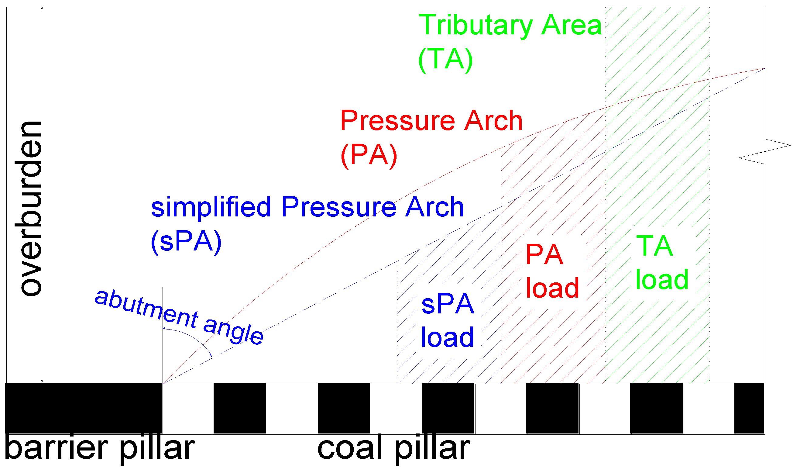
One of the site conditions that may limit the theoretical design methods is the site topography. For instance, large terrain deviations can result in drastically different overburden load distributions over a mine shaft. To address the effect of terrain changes to the pillar stresses, we first evaluate the stress distribution in a mine shaft: Figure 1 shows the schematic of an overburden on top of coal pillars in a mine tunnel with the stresses shown in colored lines. Critical review of the TAT method and the PAT method indicates that while TAT assumes that the overburden load is evenly shared by individual pillars (as shown in the green line in Figure 1), PAT assumes the formation of a pressure arch in the overburden that transfers most of overburden load to the boundary pillars, and the load below the pressure arch is applied to the production pillar (shown as the red line in Figure 1). As the shape of a pressure arch is not easily determinable, the pressure arch sometimes is simplified as a straight line (shown as a blue dashed line in Figure 1) with an assumed abutment angle. The blue dash line in Figure 1 represents the pillar load in such cases [2,5,10]. The abutment angle can be critical to the pillar stress distribution and has been studied by Wilson, Mark and Poulsen, etc. [2,11,12,13,14].

The TAT method may overestimate pillar stress because of the existence of arching over voided ground. Studies have shown that pillar stress is affected by the goaf size and if the ratio of goaf size to mining depth exceeds 3, the TAT method can provide a reliable estimation on pillar stress; otherwise, the TAT would overestimate the pillar stress because of the pressure arch effects [15]. However, TAT still seems to be the preferred method in pillar design as it is easily implementable and provides a relatively safe design [16].

Since conventional methods of design typically neglect the topography and assume that the mine site is flat, this may result in underestimating pillar stress in mountainous mining areas. In the literature, several works have already shown that the existence of a valley or a slope on top of the mine area can lead to high stress concentrations in the mines [17,18,19,20]. While most research works have focused on single pillar responses [21,22], only limited studies have addressed the state of the entire coal field due to terrain effects. For mine subsidence, Gao et al. [23] have used UDEC to evaluate the caving characteristics. The concentrated stress primarily affects the stability of the roof and pillars beneath the slope toes, and the magnitude of the stress is determined by the slope angle, the mining depth at slope bottom, and the valley width, etc. [20]. The concentrated stress can be severely large in some circumstances, such as for the shallow mining depth at the valley bottom or underneath a large slope angle. A classic case was reported by Molinda et al. [18,19]: The BethEnergy Mine 132 in West Virginia suffered a large, concentrated stress induced by a valley. The average mining depth at the valley bottom is 50 m and the smallest mining depth is only 6 m. Mining at such a shallow depth with a valley above the mine resulted in a large horizontal stress and extensive roof falls occurred. The concentrated stresses beneath a slope toe were observed by similar material experiments. Although the extreme mining conditions are very rare, the topographical effects should still be studied for a safer pillar design.

In summary, current TAT and PAT theories underestimate the pillar stress under mountainous areas due to the neglect of terrain effects. Even though terrain-induced stress concentration has been well recognized, the mechanism of stress concentration has not been explained by current theories, and stress evolution under mountainous terrain is still unclear. Furthermore, the difference and applicability of TAT and PAT are not fully discussed yet, making it hard to quantitatively decide when to use TAT or PAT. To overcome these limitations, about 1200 two-dimensional numerical models were built in order to investigate the topographical effects on pillar stresses. The full evolution of pressure arch under different terrains is exhibited and discussed, based on which the applicability of TAT and PAT is confirmed, and a modified pillar stress estimation is proposed for pillar design with topographical effects.

2. Numerical Simulation and Data Processing

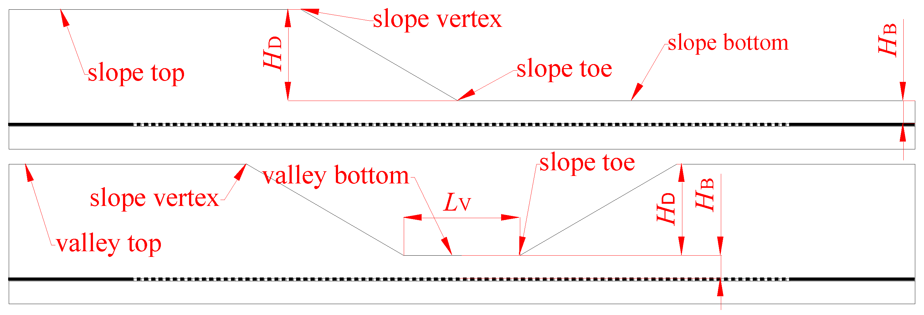
In this study, numerical modeling was performed using the Universal Distinct Element Code (UDEC, version 4.0). Two types of terrains were modeled: a single slope and a valley (two slopes) (Figure 2). The model length, floor thickness, and coal seam thickness were kept as constants and were 2000 m, 50 m, and 6 m, respectively. The variables considered include mining depth at slope bottom $H_{\mathrm{B}}$ (10–150 m), the slope height $H_{\mathrm{D}}$ (100–500 m), and the slope angle $\alpha$ (15°–90°). The valley width $L_{\mathrm{V}}$ was between 16–256 m for the valley terrain model.

All models were excavated initially at the center of the model and then extended symmetrically toward the outer boundaries until the goaf size exceeded 1500 m. With pillar width $w_{\mathrm{P}}$ ranging between 6–20 m and the ratio of mining width to pillar width $r_{\mathrm{m}}$ ranging from 0.5 to 1.75, the mining width $w_{\mathrm{C}}$ can be determined. Simplified models with deformable blocks that consist of triangular zones were built. The non-coal strata were defined as a uniform rock mass without joints. The element sizes of non-coal strata and coal seams were 4 m and 1 m, respectively. Every pillar contained an observation point located at the pillar center.

Mohr-Coulomb and Coulomb slip criterions were assumed for blocks and joints, respectively. Strata and coal properties used in the models are listed in

Table 1. Mechanical properties of the strata: ${\sigma }_{\mathrm{T}}$ is tensile strength, $c$ is cohesion, $\phi$ is internal friction angle, E is elastic modulus, $\upsilon$ is the Poisson’s ratio, and $\rho$ is density.

Rock Type	${\mathit{\sigma }}_{\mathit{T}}$ (MPa)	$\mathit{c}$ (MPa)	$\mathit{\phi }$ (°)	E (GPa)	$\mathit{\upsilon }$	$\mathit{\rho }$ (kg/m3)
non-coal strata	6.36	11.6	34.6	2–100	0.1–0.49	2500
Coal seam	0.72	2.61	42	2.2	0.27	1400

. The joint stiffness $s_{\mathrm{j}}$ between coal and non-coal strata was 5 GPa, and the strength parameters of the interfaces were matched to the coal strength. The boundary condition of the model is specified as the following: the base was fixed in the vertical direction and the lateral boundary of the model was fixed in the horizontal direction. Static equilibrium analysis was conducted with consideration of gravitational loads on the model. The specific values of the variables for simulations (e.g., $H_{\mathrm{B}}$, $H_{\mathrm{D}}$, E, etc.) were further described in the corresponding case studies below, and the UDEC codes for simulations refer to Supplementary Materials 1–5.

The vertical stress on each pillar was recorded after the simulation. To compare the simulated pillar stress $S_{\mathrm{S}}$ and the theoretical pillar stress $S_{\mathrm{T}}$ estimated by TAT, the stress variation coefficient $K$ is defined as:

$$K=\frac{S_{\mathrm{S}}}{S_{\mathrm{T}}}$$

(1)

where $K>1$ indicates that the TAT underestimated the pillar stress, and $K<1$ indicates that the TAT overestimated the pillar stress.

Figure 3 shows the schematics for the calculated $S_{\mathrm{T}}$ for the slope model: The TAT method assumed that the pillar stresses are the same under the slope top or the slope bottom, hence, the average mining depth above the pillar was used to calculate $S_{\mathrm{T}}$ (green strips) for the pillars under the slope. The $K$ of each pillar was calculated and representative simulation results were selected and illustrated in the following section (the complete analysis results and raw data for all models are available in Supplementary Materials 1–5).

3. The Effect of a Single Slope on Pillar Stress

3.1. The Effects of H_D and a on Pillar Stress

The single slope models with $H_{\mathrm{B}}$ of 10 m, $w_{\mathrm{P}}$ of 8 m, $r_{\mathrm{m}}$ of 1, E of 15 GPa, and $\upsilon$ of 0.15 were selected as the base models for the parametric analysis. The $H_{\mathrm{D}}$ of the models varied from 100–500 m and the $\alpha$ was 15°–90°. Representative simulation results are shown in Figure 4, where Figure 4a,b shows that the single slopes led to stress concentrations on the pillars directly below the slope toes (for Pillar A when $\alpha$ < 90° and for Pillar B when $\alpha$ = 90°, as indicated in Figure 3), which means that TAT may severely underestimate the pillar stress in these cases. $K$ for Pillar A or Pillar B is the maximum value on the $K$ curves, and the maximum $K$ will increase if $H_{\mathrm{D}}$ increases. Similar observations have been made by Gao et al. [23]. Figure 4c,d shows that the corresponding spatial locations of the K value where maximum $K$ is shown to increase with increasing $\alpha$. All the simulation results of the 1200 models are similar to Figure 4 and have the same observations: The maximum $K$ appears in Pillar A ($\alpha$ < 90°) or Pillar B ($\alpha$ = 90°), and the maximum $K$ increases with $H_{\mathrm{D}}$ or $\alpha$ increase.

Another observation is that the $K$ under the slope top or the slope bottom is close to a value of 1 and that the $K$ below the slope top is usually smaller than the $K$ beneath the slope bottom ($K$ beneath the slope bottom may be slightly larger than 1, Figure 4d). This may suggest that the pillar stress below the slope bottom may be slightly underestimated by the TAT method.

Finally, due to the pressure arch effects, the $K$ curves beneath the slope top or slope bottom become ripple-like when $H_{\mathrm{D}}$ is small (Figure 4b), where the overburden load is transferred to different pillars by a series of pressure arches [5,24]. The stress increases when an arch foot is on top of a pillar, and the stress decreases when the arch top lies on a pillar. The corresponding portion in the $K$ curves in Figure 4a are also ripple-like.

In general, the TAT method is suitable for pillar stress calculation if we can appropriately deal with the stress concentration around the slope toe. By using $K_{\mathrm{m}}$ to represent the maximum simulated concentrated stress, the effects of E, $\upsilon$, $H_{\mathrm{B}}$ are then studied.

3.2. The Effect of Rock Properties on Pillar Stress

To study the effect of rock properties, $\upsilon$ was varied from 0.1 to 0.49 and E was kept as constant at 15 GPa. To study the effect of E, it is varied from 2 GPa to 100 GPa, while $\upsilon$ was kept at 0.15. The other parameters were fixed as mentioned in Section 3.1. Figure 5 shows that when $H_{\mathrm{D}}$ is small, $\upsilon$ has little effect on $K_{\mathrm{m}}$. Figure 6 shows that the increase in E has significantly increased $K_{\mathrm{m}}$ (Figure 6), which means that the stress concentration will be more severe if the overburden consists of hard rocks.

3.3. The Effect of H_B on Pillar Stress

To study the effect of $H_{\mathrm{B}}$ on pillar stress, $H_{\mathrm{B}}$ was set at 30 m, 50 m, 80 m, 100 m, 150 m, respectively, and the other parameters were fixed as described in Section 3.1. Figure 7 shows that if $H_{\mathrm{B}}$ is increased, the value of $K_{\mathrm{m}}$ is decreased. However, the influence of $K_{\mathrm{m}}$ is widened as $H_{\mathrm{B}}$ increases (in other words, the number of pillars that are suffering concentrated stresses will increase). This implies that $H_{\mathrm{B}}$ plays a very important role in the load transfer from the overburden to the pillars.

The relationship between $H_{\mathrm{B}}$ and pressure arch is key in explaining the stress concentration induced by the topography: The overburden load above a pillar can be transferred to further-located pillars by pressure arches [2,5,24,25]. If $H_{\mathrm{B}}$ is large, there will be enough space to form large pressure arch structures, and the overburden loads can be transferred to the further-located pillars and shared by more pillars. Because the formation of the pressure arch is constrained (for small $H_{\mathrm{B}}$) by the boundary conditions and rock properties, the transfer of the overburden is limited. For a single slope model, the overburden thickness decreases around the slope toe, so the load transfer by pressure arch is disrupted in such a way that most of the overburden loads will act on the pillar that is directly beneath the slope toe (i.e., Pillar A shown in Figure 3). As shown in Figure 3, Pillar A behaved like the arch foot where an extremely large $K_{\mathrm{m}}$ appeared due to the load transfer and was restricted by a small pressure arch that was induced by the small $H_{\mathrm{B}}$. However, the pressure arch can be larger when $H_{\mathrm{B}}$ increases, so the overburden loads can be transferred further and shared by more pillars, and the $K_{\mathrm{m}}$ thus decreases.

More evidence is shown in Figure 8 that when $H_{\mathrm{B}}$ is small, $K_{\mathrm{m}}$ is large and less pillars are affected by the concentrated stresses indicating that the pressure arches under the slope bottom fail to transfer the overburden loads further. When $H_{\mathrm{B}}$ is large, the $K_{\mathrm{m}}$ is very small and more pillars are affected by the concentrated stresses, indicating that a large $H_{\mathrm{B}}$ can result in a large pressure arch, and the overburden loads can be transferred further and shared by more pillars.

Analysis shows that the concentrated stresses only occur at a limited distance: $K$ started to increase at a slope vertex (Pillar C in Figure 3) and reached a maximum value at a slope toe. We can then define an influence range, $L_{\mathrm{I}}$, where the $K$ decreases. $L_{\mathrm{I}}$ is affected by $H_{\mathrm{B}}$ and can be roughly estimated as:

$$L_{\mathrm{I}}=0.8H_{\mathrm{B}}+37$$

(2)

where $L_{\mathrm{I}}$ is the influence range of concentrated stress at slope bottom, m.

3.4. The Effects of w_p and r_m on Pillar Stress

To study the effect of $w_{\mathrm{P}},w_{\mathrm{P}}$ was varied from 6 m to 20 m and $r_{\mathrm{m}}$ was fixed as 1. To study the effect of $r_{\mathrm{m}}$, $r_{\mathrm{m}}$ was varied from 0.5 to 1.75 and $w_{\mathrm{P}}$ was fixed at 8 m. Other parameters are fixed as mentioned in Section 3.1.

Figure 9 shows that $K_{\mathrm{m}}$ decreases with increasing $w_{\mathrm{P}}$ or $r_{\mathrm{m}}$. It seems that a large pillar with a large mining width is more capable of reducing stress concentration and improving the accuracy of TAT. This is because: (1) A large $w_{\mathrm{P}}$ or $r_{\mathrm{m}}$ means a large $w_{\mathrm{C}}$. As the shape of the pressure arch is controlled by $w_{\mathrm{C}}$, a large $w_{\mathrm{C}}$ creates a large pressure arch [5,24,25]. If $w_{\mathrm{C}}$ is small, it is hard to form pressure arches and trigger the load transfer that leads to a large $K_{\mathrm{m}}$; and (2) the pillar stress is not uniformly distributed. It is, therefore, concluded that the stress at pillar center decreases with the increase of $w_{\mathrm{P}}$.

Finally, mining with large $w_{\mathrm{C}}$ and large $w_{\mathrm{P}}$ can reduce pillar stress concentration and improve pillar safety. However, the ground subsidence is also controlled by $w_{\mathrm{C}}$, which when failing may result in roof failure (if the $w_{\mathrm{C}}$ is too large) [26,27]. A balance should, therefore, be made between ground subsidence control and pillar stress control.

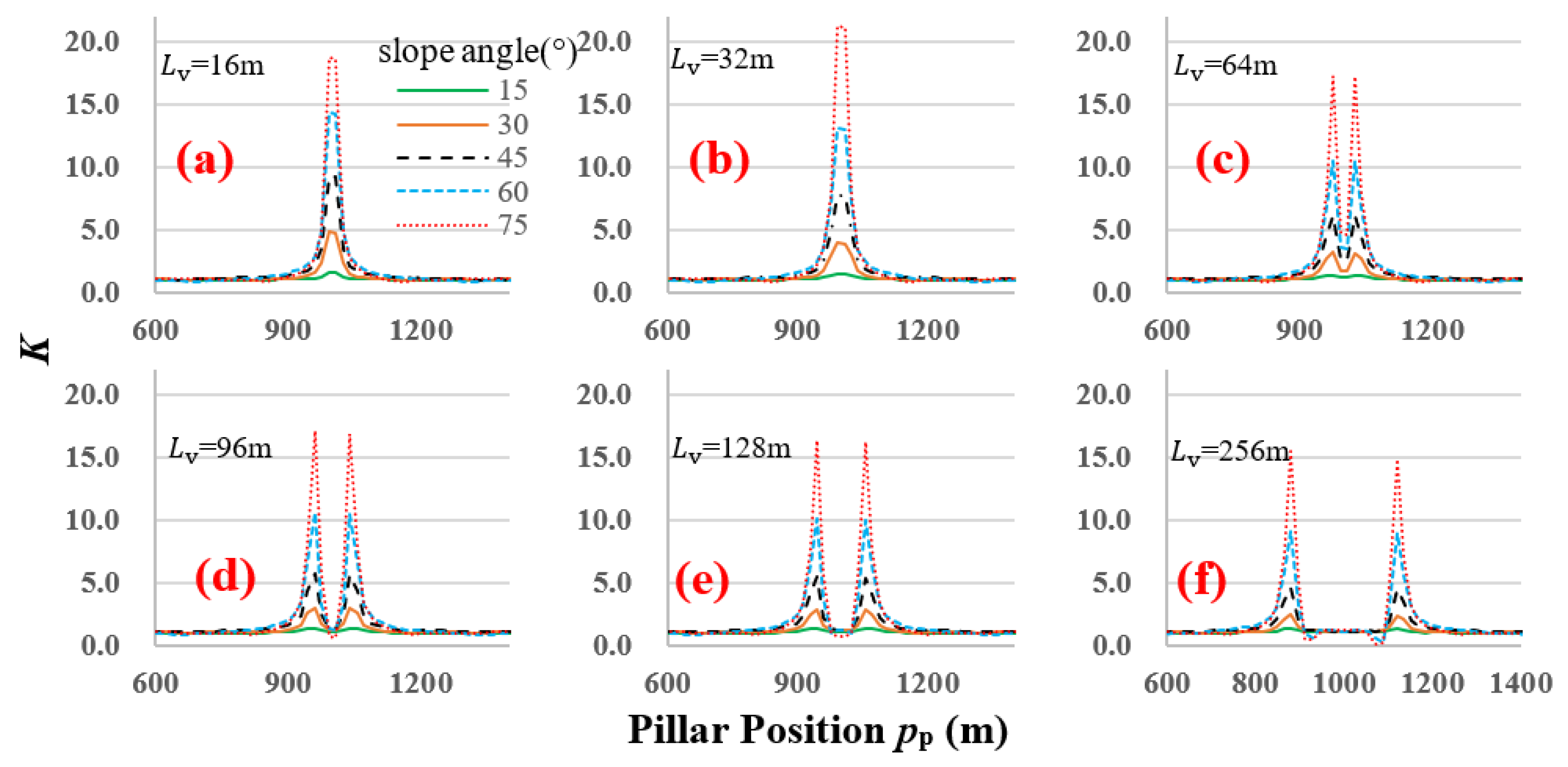
4. The Effect of a Valley on Pillar Stress

A valley ground surface is a combination of two single slopes facing each other, where stress concentrations will occur for the valley terrain. Since $K_{\mathrm{m}}$ has been used to represent the maximum $K$ for a single slope terrain, to make a distinction, $K_{\mathrm{vm}}$ is used to represent the maximum $K$ for a valley terrain. The $H_{\mathrm{B}}$ is fixed at 10 m to study the maximum $K_{\mathrm{vm}}$ for the valley terrain. The other parameters remained fixed as described in Section 3.1. The valley width $L_{\mathrm{v}}$ varied from 16 m to 256 m. 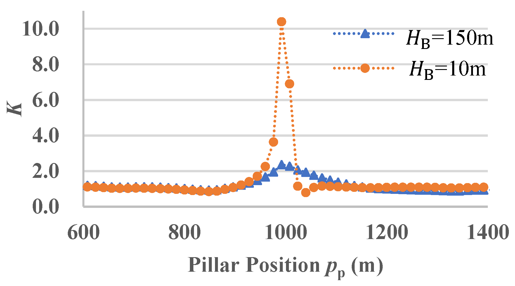Figure 10 shows the distribution of $K_{\mathrm{vm}}$ for the valley models.

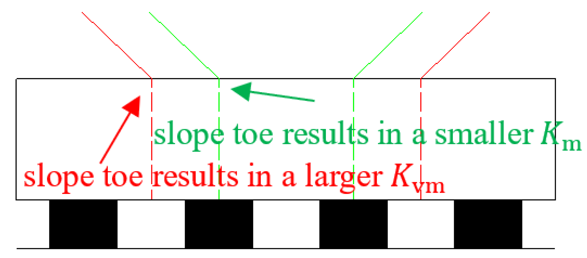
Due to the superimposed effects of the two slopes, $K_{\mathrm{vm}}$ is larger than $K_{\mathrm{m}}$, and there are two $K_{\mathrm{vm}}$ of equal values beneath the slope toes of the valley. $K_{\mathrm{vm}}$ decreases with increasing $L_{\mathrm{v}}$ and reaches a constant value. In addition, it was also found that $K_{\mathrm{vm}}$ will be larger if the slope toe lies between two adjacent pillars (the red lines in Figure 11) instead of lying directly above a pillar (the green lines in Figure 11). It is better to ensure that the slope toes lie directly above a pillar when conducting a pillar design to reduce the stress concentration.

5. Discussion

5.1. Mechanism of Pillar Stress Concentration Induced by Terrain

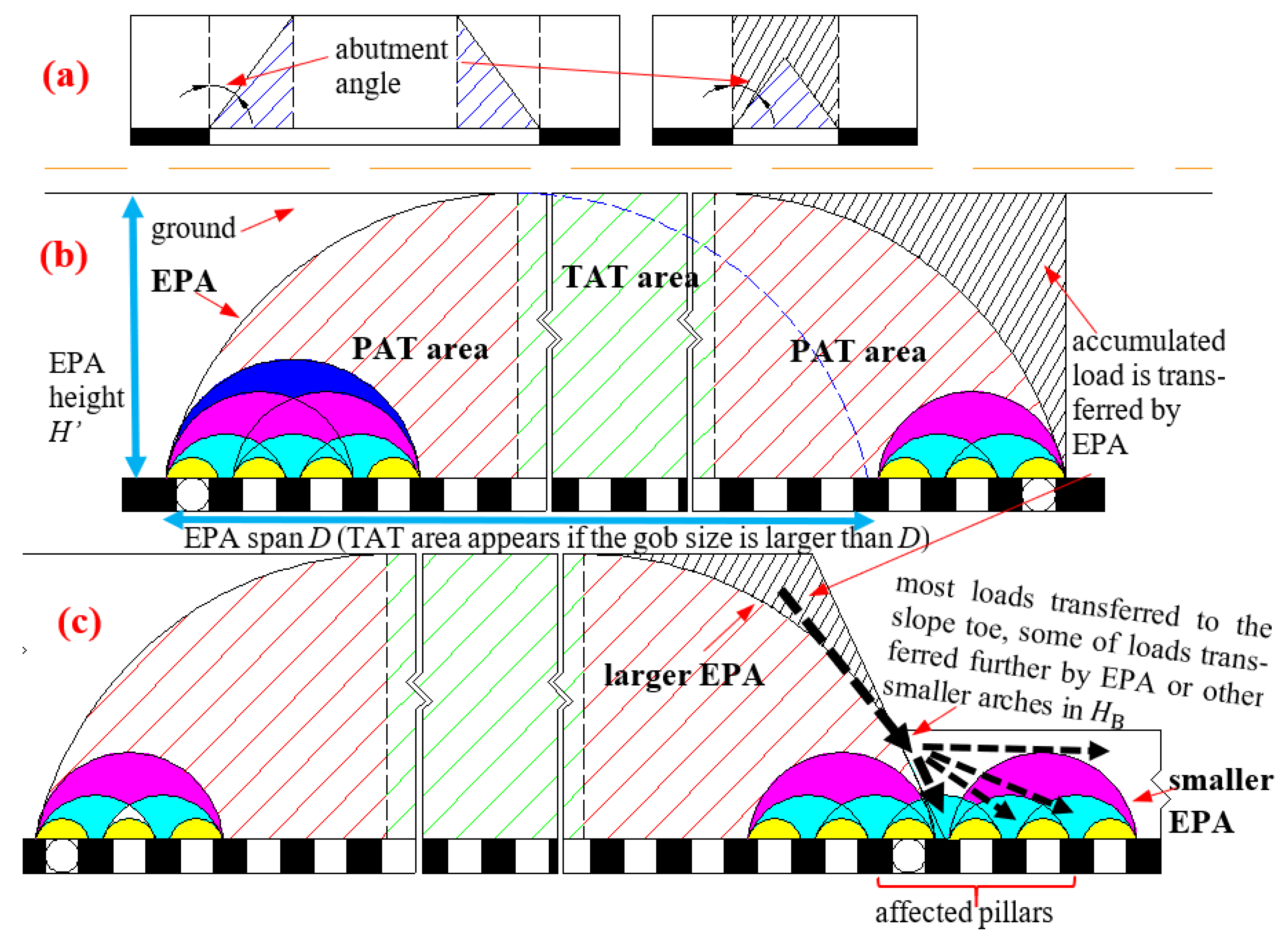
For a horizontal and flat ground surface, both TAT and PAT are capable of calculating the pillar stresses. TAT may overestimate the pillar stress when the gob size is small because it ignored the pressure arch effects in the overburden rock mass [2,5,10,11,12,15,24,25]. Pressure arch exists when a deposit is extracted regardless of the overburden rock types or the mining methods [2,11,28,29]. When a continuous void space is created by longwall mining, the line determined by the abutment angle can actually be treated as a simplified pressure arch (i.e., the blue area in Figure 12a), and the overburden load in the range of the abutment angle is transferred to the boundary pillars [2,11,12,13,14]. When a small tunnel is created, a small pressure arch also known as the Protodyakonov’s equilibrium arch, forms above the voided mine space (the yellow area in Figure 12b), and many Protodyakonov’s equilibrium arches will merge into larger arches (the cyan and magenta areas in Figure 12b) when more excavated tunnels are formed [5,24,29]. The continuous mining gradually expands Protodyakonov’s equilibrium arches to a large extended pressure arch (EPA in Figure 12b) [5,24]. The height and influenced area of EPA gradually expands with the increase of gob size, and finally, the overburden loads above EPA will be continuously transferred away from the gob.

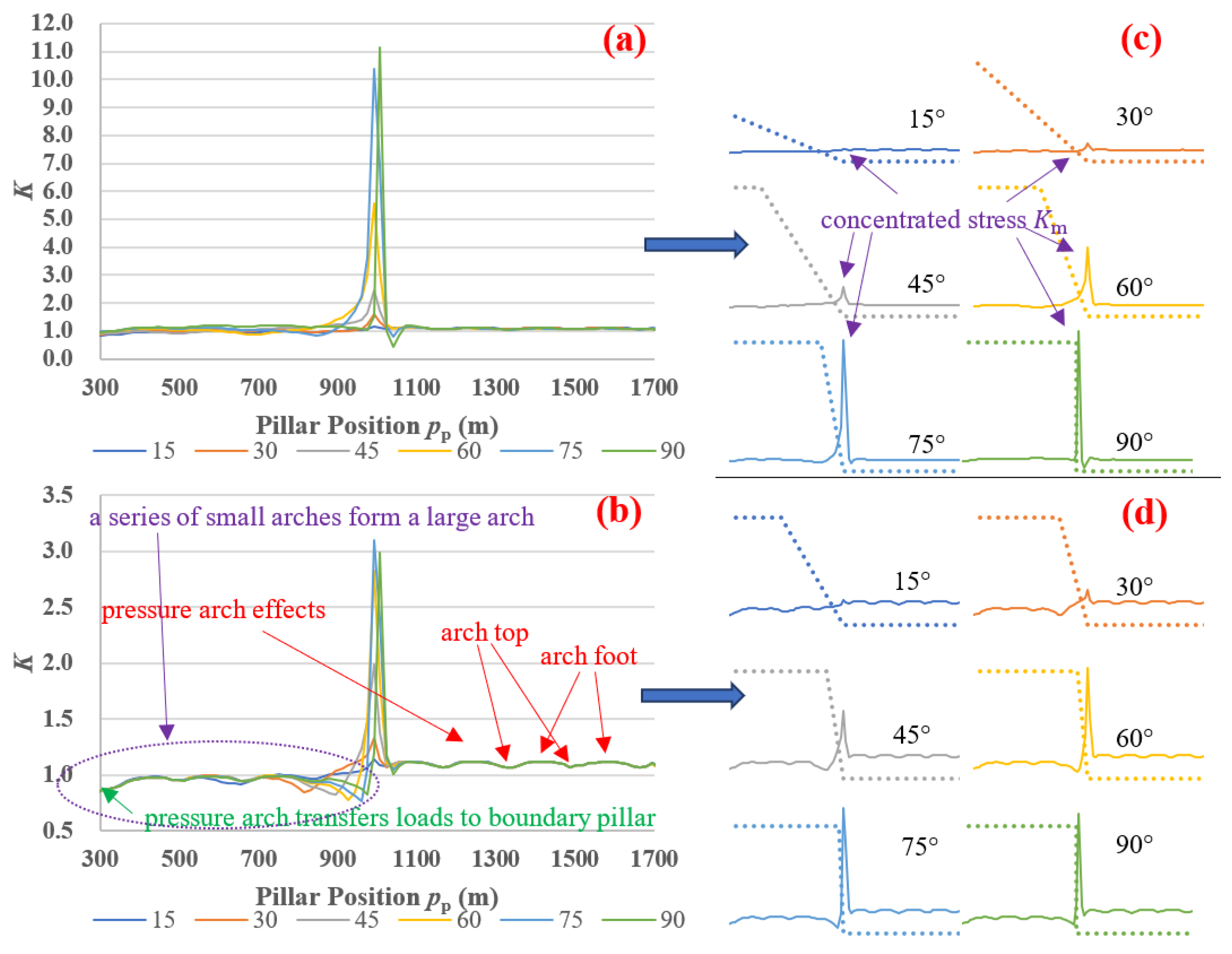
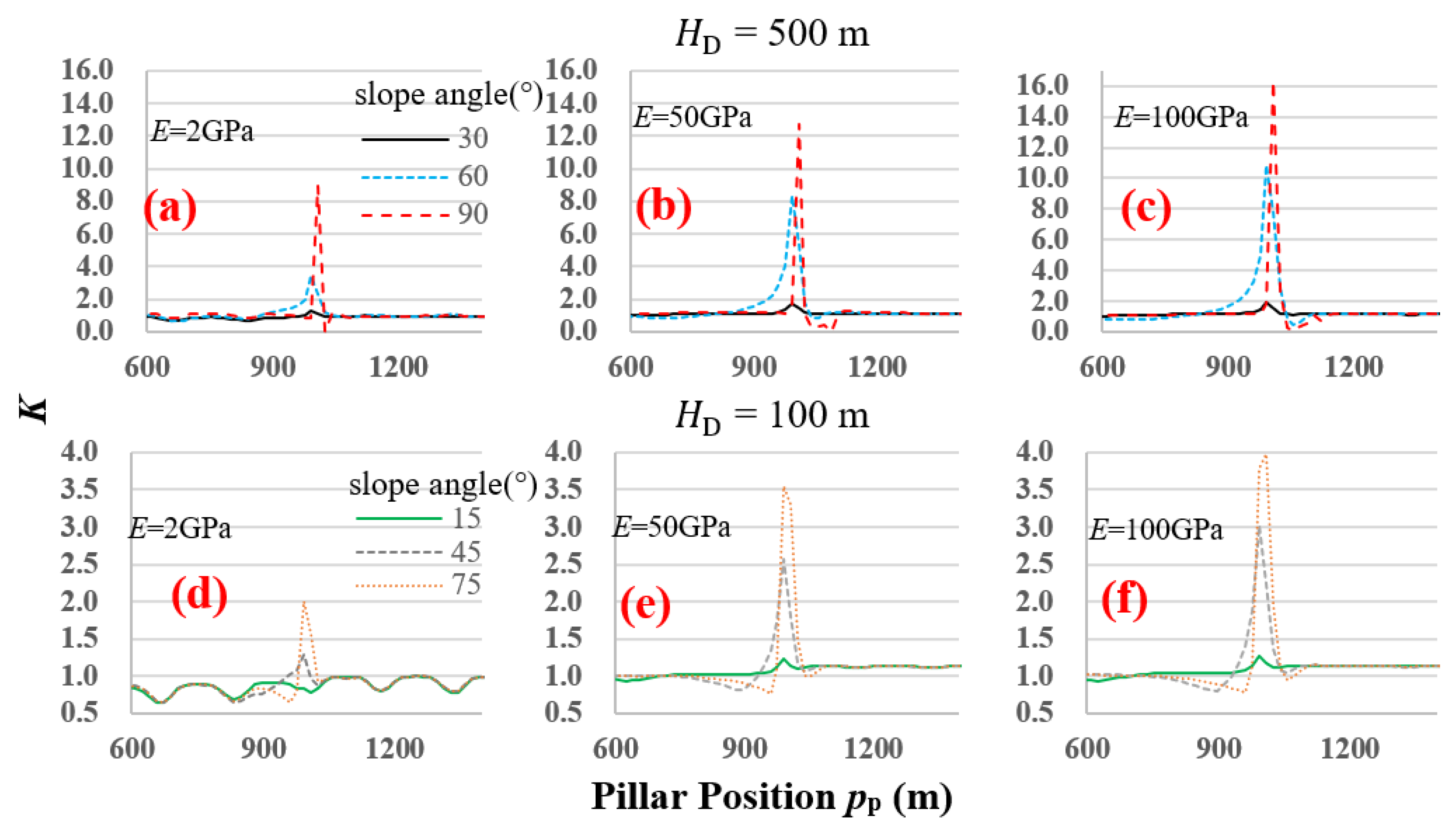
However, the expansion of EPA is not endless. When the gob size is large enough, EPA will reach the ground surface and the pressure arch structures turn into a half-arch and half-beam structure. Thus, the overburden can be divided into PAT affected areas (the areas with red dashed lines in Figure 12b) and TAT affected area (areas with green dashed lines in Figure 12b). Only the loads above EPA can be transferred to the boundary pillars. This is why the TAT can provide a reliable pillar estimation when the gob is large but overestimate the pillar stress when the gob is small. Evidence can also be found from multiple figures in this paper, e.g., in Figure 4, the $K$ at slope bottom or slope top is always near one, indicating that the stress estimated by TAT is accurate in the TAT area; the $K$ at slope bottom or slope top is ripple-like, indicating that some small pressure arches redistribute the overburden stress, and the EPA is a macro arch that consists of micro arches; and finally, a large pressure arch that is composed of many small pressure arches reduces pillar stress near the gob boundary.

On mountainous terrain, the EPA formation is disturbed by the variation of topography, and the load transfer mechanism is shown in Figure 12c, where a large EPA is formed ($H_{\mathrm{D}}$ is sufficiently large) which transfers the strata loads away from the gob. When the $H_{\mathrm{B}}$ is smaller, the EPA at slope (or valley) bottom is small and has less overburden load to transfer. It is suggested that the smaller the $H_{\mathrm{B}}$ is, the smaller the EPA will be, and the less overburden load it will transfer. As a result, more overburden load is transferred to the slope toe by the larger EPA in $H_{\mathrm{D}}$, and less overburden load is transferred away from the slope toe by the smaller EPA in $H_{\mathrm{B}}$, thus, leading to a severe stress concentration around the slope toe. If $H_{\mathrm{B}}$ is larger, EPA at slope bottom will be enlarged and can transfer the load further and more loads will be transferred away.

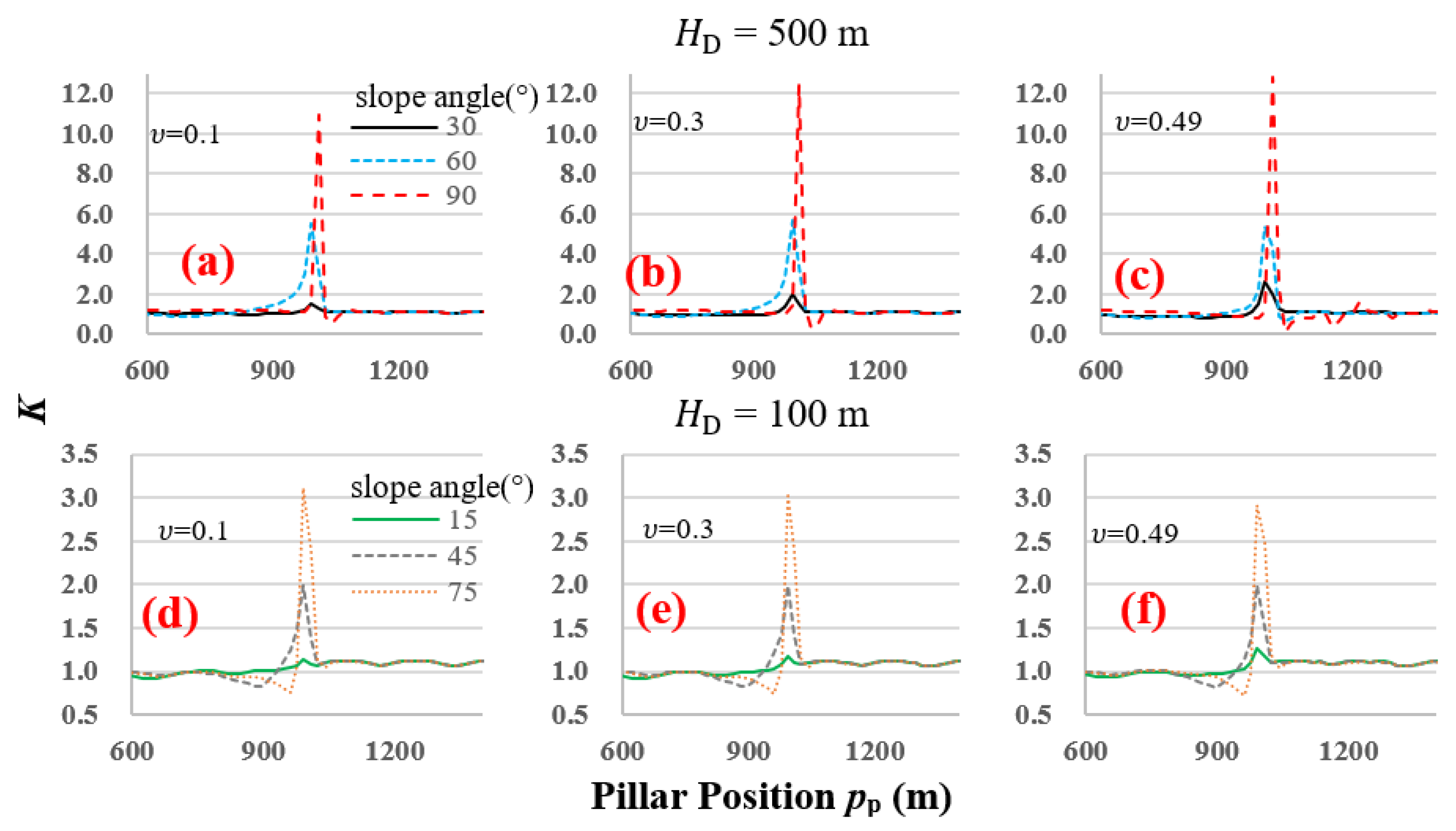
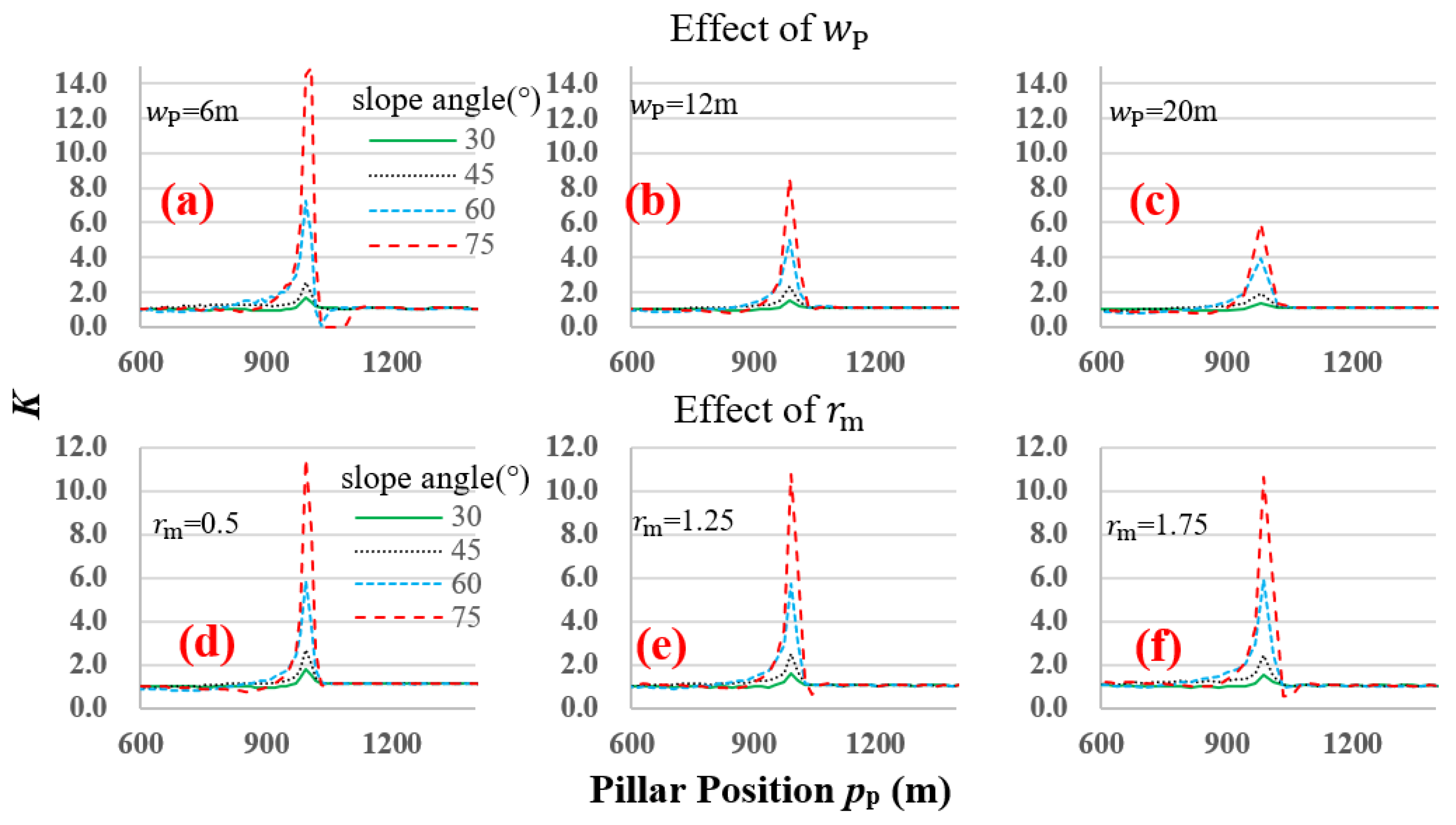
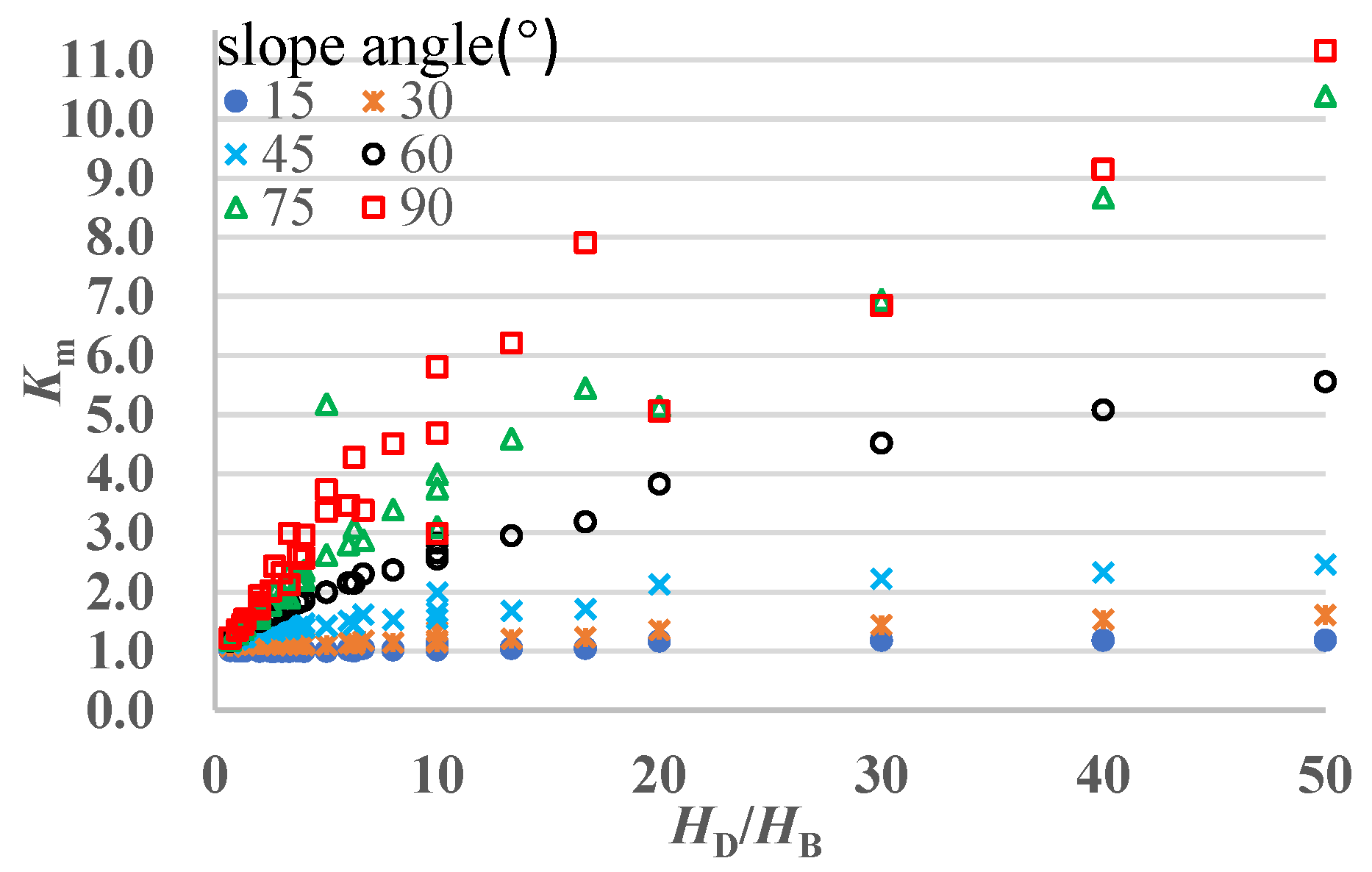
Figure 13 shows that $K_{\mathrm{m}}$ will decrease if $H_{\mathrm{D}}/H_{\mathrm{B}}$ or $\alpha$ decreases. A smaller $\alpha$ or $H_{\mathrm{D}}/H_{\mathrm{B}}$ means that the topographical variation is gentle, making EPA decrease smoothly from slope top to slope bottom and reduce the stress concentration. Therefore, it is the intensity of the EPA variation, instead of the mining depth, the slope height, or other factors, that controls the stress concentration. As long as there is a drastic change in EPA by the site topography, there will be stress concentrations. Regression analysis in Figure 13 indicates that the topographical influence of $H_{\mathrm{D}}/H_{\mathrm{B}}$ on $K_{\mathrm{m}}$ is limited to $\alpha <$23°.

In brief, a mountainous terrain leads to stress concentrations in pillars; the concentrated stresses are near the slope toe and result from the variation of EPA. As the variation of EPA is not fully considered in current TAT and PAT methods, they may have limitations and cannot be directly used in mountainous areas.

5.2. Pillar Stress Calculation for a Horizontal Ground

Studies show that the pressure arch is affected by gob size, mining depth, cave width, rock properties, etc. [5,24,25,29,30,31]. While it is difficult to determine the accurate shape of the pressure arch, it is possible to assume the approximate shape of an EPA for a horizontal ground by:

$$\frac{D}{H^{\prime }}=\frac{2f}{k}$$

(3)

where $D$ is the span of EPA, m; $H^{\prime }$ is the height of EPA, m and $f$ is the Protodyakonov coefficient of overburden (equal to 1/10 of uniaxial compressive strength of overburden in MPa). $k$ is the pressure arch correction coefficient and is defined as:

$$k=\{\begin{array}{c}4.0-5.0, f\le 0.8\\ 3.0-4.0, 0.8<f\le 4\\ 1.5-2.0, 5<f\le 8\end{array}$$

(4)

Considering Equations (3) and (4), the maximum pillar stress $P$ can be calculated as:

$$P=\frac{\left(w_{\mathrm{P}}+w_{\mathrm{C}}\right)\rho g{H}^{\prime }}{w_{\mathrm{P}}}$$

(5)

If the mine size is larger than $D$, the EPA reaches the ground surface and $H^{\prime }$ equals the mining depth. In such situations, Equation (5) is the same as the TAT method.

Equations (3)–(5) and EPA can also be supported by the literature [15]. The TAT method has been found to provide a good estimation of the pillar stress if the ratio of goaf size to mining depth exceeds 3–4, otherwise the method overestimates the pillar stress [15]. This observation can be explained by the EPA theory: If ${\sigma }_{\mathrm{C}}$ of 11.6 MPa and $\phi$ of 34.6° were used as the overburden properties, the uniaxial compressive strength of overburden ${\sigma }_{\mathrm{u}}$ can be computed as:

$${\sigma }_{\mathrm{u}}=\frac{2{\sigma }_{\mathrm{C}}\cos \phi }{1-\sin \phi }$$

(6)

The result is 44 MPa. Therefore, setting $k$ in Equation (4) as 2–3, and $D/H^{\prime }$ in Equation (3) as 2.9–4.4 (meaning that the EPA reached the ground surface), the ratio of the goaf size to mining depth will exceed 2.9–4.4 (close to Yu’s ratio of 3–4). So, the mine size effect on pillar stress essentially resulted from EPA, and TAT provides a reliable stress calculation after EPA reaches the ground surface.

5.3. Pillar Stress Calculation for a Mountainous Terrain

For a mountainous terrain, the variation of EPA is more complicated and an alternative pillar stress estimation method is proposed: (1) The stress of each pillar can be calculated by TAT; (2) $K_{\mathrm{m}}$ or $K_{\mathrm{vm}}$ can be used to correct the pillar stress at the slope toe; and (3) when a pillar is located away from the slope toe, its $K$ decreases from $K_{\mathrm{m}}$ or $K_{\mathrm{vm}}$ to 1. The decrease in K can be represented by a linear function because the $K$ curve is concave. $K$ for different pillars can be calculated and used to correct the stresses of remnant pillars, and the actual stress of an individual pillar $P_{\mathrm{i}}$ can be estimated by:

$$P_{\mathrm{i}}=K_{i}P$$

(7)

where $K_i$ is the $K$ for an individual pillar, $K_i$ can be estimated as long as $K_{\mathrm{m}}$ or $K_{\mathrm{vm}}$ is acquired; $P$ is pillar stress calculated by Equation (5), $H^{\prime }$ in Equation (5) should be the average mining depth above a pillar.

5.3.1. Calculation of K_m and K_mv

$K_{\mathrm{m}}$ for the single slope (base) models functions of $H_{\mathrm{D}}$ and $\alpha$ and can be estimated as:

$$\begin{gathered} K_{\mathrm{m}-\mathrm{base}}=\left(-4.024\times {10}^{-7}{\alpha }^3+7.741\times {10}^{-5}{\alpha }^2-4.565\times {10}^{-3}\alpha + \\ 0.1051\right)H_{\mathrm{D}}-0.8025H_{\mathrm{D}}/\alpha +1.488 \end{gathered}$$

(8)

where $K_{\mathrm{m}-\mathrm{base}}$ is the $K_{\mathrm{m}}$ for base models; the Root Mean Squad Error (RMSE) is 0.27 and the R² is 0.9918.

Parametric analysis was performed on $K_{\mathrm{m}}$ and resulted in the following equation for calculating $K_{\mathrm{m}}$ after a single mining condition change:

$$K_{\mathrm{m}-i}=K_{\mathrm{m}-\mathrm{base}}\left(1+{\Delta }_i\right)$$

(9)

where $K_{\mathrm{m}-i}$ is the $K_{\mathrm{m}}$ after a particular mining condition is changed and $i$ is the mining condition such as E, $\upsilon$, $H_{\mathrm{B}}$. For example, $i=\upsilon$ means $\upsilon$ is changed; $K_{\mathrm{m}-\mathrm{base}}$ is the $K_{\mathrm{m}}$ for base models; ${\Delta }_i$ is the variation rate of $K_{\mathrm{m}-\mathrm{base}}$ that is induced by the changing of a mining condition $i$.

If multiple mining condition changes are involved, $K_{\mathrm{m}}$ can be determined by:

$$K_{\mathrm{m}-i}=K_{\mathrm{m}-\mathrm{base}}\prod \left(1+{\mathsf{\Delta }}_i\right)$$

(10)

To study the effect of the Poisson’s Ratio, statistics analysis shows that ${\Delta }_i$ for different mining conditions can be estimated by:

$${\mathsf{\Delta }}_{\upsilon }=3.298{\nu }^{2.295}\left(15.28-8.614\sin 5.489\alpha -18.46\cos 5.489\alpha \right)/\alpha$$

(11)

where ${\mathsf{\Delta }}_{\upsilon }$ is the variation rate of $K_{\mathrm{m}-\mathrm{base}}$ due to $\upsilon$ variation; the RMSE is 0.02908 and the R² is 0.963.

To study the effect of the elastic modulus, statistics analysis shows that ${\Delta }_i$ can be estimated by:

$$\begin{gathered} {\mathsf{\Delta }}_E=\left(0.03852E^{0.5337}-0.1552\right)\left[0.7676\sin \left(6.097\alpha -3.921\right)+ \\ 2.846\sin 1.359\alpha \right] \end{gathered}$$

(12)

where ${\mathsf{\Delta }}_E$ is the variation rate of $K_{\mathrm{m}-\mathrm{base}}$ with different $E$; the RMSE is 0.0367 and the R² is 0.988.

To study the effect of different $H_{\mathrm{B}}$, a correlation equation for ${\Delta }_i$ is determined as:

$${\mathsf{\Delta }}_{\mathrm{B}}=\left(0.57{\mathrm{e}}^{-0.04379H_{\mathrm{B}}}-0.3705\right)\left[1-0.6733\sin \left(2.353-3.044\alpha \right)\right]$$

(13)

where ${\mathsf{\Delta }}_{\mathrm{B}}$ is the variation rate of $K_{\mathrm{m}-\mathrm{base}}$ when $H_{\mathrm{B}}$ is changed; the RMSE is 0.02992 and the R² is 0.9798.

To study the effect of $w_{\mathrm{P}}$, statistics analysis shows that ${\Delta }_i$ can be estimated by:

$${\mathsf{\Delta }}_{\mathrm{p}}=0.6814{\mathrm{e}}^{0.03723\alpha }\left(0.5075{\mathrm{e}}^{-0.3228w_P}-0.03182\right)$$

(14)

where ${\mathsf{\Delta }}_{\mathrm{p}}$ is the variation rate of $K_{\mathrm{m}-\mathrm{base}}$ when $w_{\mathrm{P}}$ is changed; the RMSE is 0.05177 and the R² is 0.9584.

Finally, to study the effect of $r_{\mathrm{m}}$, statistics analysis shows that ${\Delta }_i$ can be estimated by:

$${\mathsf{\Delta }}_r=\left(0.066{\mathrm{e}}^{-1.265r_{\mathrm{m}}}-0.01883\right)\left(1.664\times {10}^{-6}{\mathrm{e}}^{0.1822\alpha }+1\right)+0.04187/r_{\mathrm{m}}$$

(15)

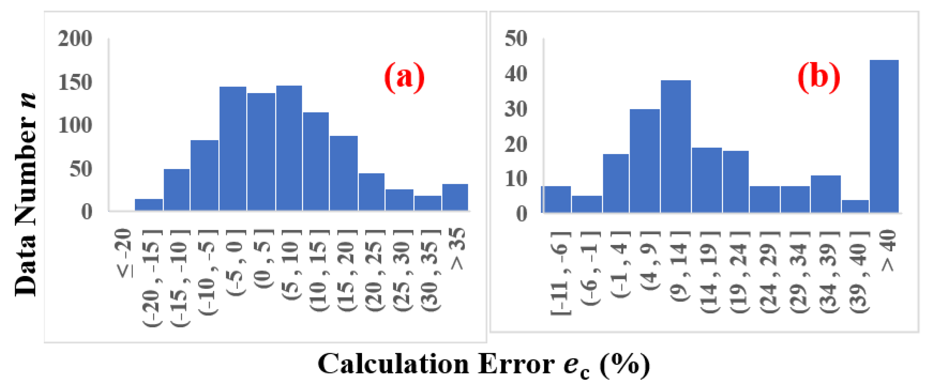
where ${\mathsf{\Delta }}_r$ is the variation rate of $K_{\mathrm{m}-\mathrm{base}}$ when $r_{\mathrm{m}}$ is changed; the RMSE is 0.02892 and the R² is 0.9281. As stated earlier, $K_{\mathrm{m}}$ for a single slope model can be estimated by Equation (10), an error analysis is conducted, and the results are presented in Figure 14a.

We then proceed to analyze the valley models by comparing $K_{\mathrm{vm}}$ with $K_{\mathrm{m}-\mathrm{base}}$. Under the same mining conditions, $K_{\mathrm{vm}}$ for a valley model is larger than the $K_{\mathrm{m}-\mathrm{base}}$ for a single slope model. Although a valley is a combination of two single slopes into one terrain, a valley effect is not a linear superposed effect of the two slopes, and $K_{\mathrm{vm}}$ is not the sum of $K_{\mathrm{m}-\mathrm{base}}$ from two slopes. As a matter of fact, $K_{\mathrm{vm}}$ can be about four times larger than $K_{\mathrm{m}-\mathrm{base}}$, and the valley effects on EPA are more complicated.

Considering the most unfavorable conditions, it is found that $K_{\mathrm{vm}}$ can be estimated by:

$$\begin{gathered} K_{\mathrm{mv}}=\left[\left(7.368\times {10}^{-8}{\alpha }^3-1.409\times {10}^{-5}{\alpha }^2+7.677\times {10}^{-4}\alpha - \\ 0.007896\right)H_{\mathrm{B}}+1.043\right]K_{\mathrm{m}-\mathrm{base}} \end{gathered}$$

(16)

The RMSE of Equation (16) is 0.1223, R² is 0.9687 and the calculated errors are shown in Figure 14b. Figure 14 shows that $K_{\mathrm{m}}$ or $K_{\mathrm{mv}}$ will not be severely under-estimated by the proposed equations. So, for a conservative pillar design, $K_{\mathrm{m}}$ can be calculated by combining Equation (10) and $K_{\mathrm{mv}}$ can be calculated by Equation (16).

5.3.2. Stress Calculation for Individual Pillars

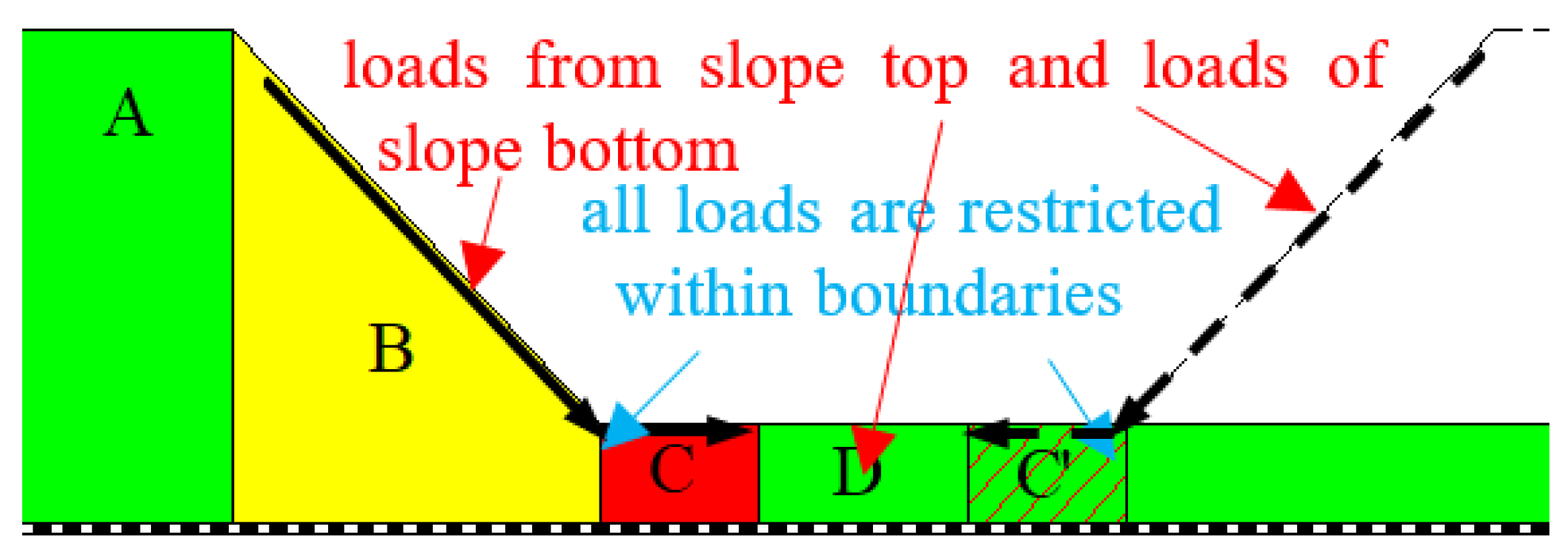
To calculate the pillar stress at different parts of mountainous terrain, a single slope model or a valley model can be divided into 4 sections (Figure 15):

(1) In sections A and D, the EPA shape is not significantly changed as the terrain is horizontal and flat. Therefore, the pillars under these sections are not affected by terrain effects, and K_i in Equation (7) is 1.

(2) In section B, the size of EPA reduces the load transfer and the load above EPA concentrated in the downhill direction. When a pillar is located from the slope vertex to the slope toe, its K increases linearly from 1 to K_m. K_i for these pillars can be estimated as:

$$K_i=\frac{x\left(K_{\mathrm{m}-i}-1\right)\tan \alpha }{H_{\mathrm{D}}}+1$$

(17)

where $x$ is the horizontal distance between the pillar and the slope vertex, m; and $K_{\mathrm{m}-i}$ is estimated by Equation (10).

(3) In section C, the EPA at slope bottom transfers part of the accumulated loads from the slope toe, making many pillars under section C bear additional stresses. When a pillar is located from the slope toe to a distance of L_I, the width of section C is L_I, and K decreases linearly from K_m to 1. K_i for these pillars is:

$$K_i=\frac{x^{\prime }\left(1-K_{\mathrm{m}-i}\right)}{L_{\mathrm{I}}}+K_{\mathrm{m}-i}$$

(18)

where $x^{\prime }$ is the horizontal distance between the pillar and the slope toe, m. $L_{\mathrm{I}}$ is the horizontal range of section C and is estimated by Equation (2).

Since there are two slopes for a valley terrain, a section C’ will be created by the opposing slope. As Sections C and C’ are mirror images of each other, two situations may exist for a valley terrain:

(a) L_v is large and Sections C and C’ are not intersected. Although the two sections are not intersecting with each other, the non-linear superposed effects of two slopes still exist, and we cannot treat a valley as two slopes and calculate the pillar stress separately. For example, the distance between C and C’ is 108 m when $L_{\mathrm{v}}=$208 m, even though the two slopes are significantly apart, $K_{\mathrm{vm}}$ is twice larger than $K_{\mathrm{m}}$. This is because there is another slope in existence that is restricting the load transfer beneath the slope bottom.

If there only exists a single slope, the accumulated loads from the slope top can be partially transferred to the gob edge by EPA of the slope bottom. While the additional slope not only brings additional loads to the slope bottom, it also interrupts the load transfer. The two pillars beneath the slope toes are like two boundaries and all the loads were restricted at the slope bottom, leading to a more severe stress concentration.

Hence, for a valley terrain, $K_{\mathrm{vm}}$ instead of $K_{\mathrm{m}-i}$ should be used to calculate $K_i$. $K_i$ for section B is:

$$K_i=\frac{x\left(K_{\mathrm{vm}}-1\right)\tan \alpha }{H_{\mathrm{D}}}+1$$

(19)

where $x$ is the horizontal distance between the pillar and the slope vertex, m; $K_{\mathrm{vm}}$ is estimated by Equation (16). $K_i$ for section C is calculated as:

$$K_i=\frac{x^{\prime }\left(1-K_{\mathrm{vm}}\right)}{L_{\mathrm{I}}}+K_{\mathrm{vm}}$$

(20)

where $x^{\prime }$ is the horizontal distance between the pillar and the slope toe, m. $L_{\mathrm{I}}$ is the horizontal range of section C and is estimated by Equation (16).

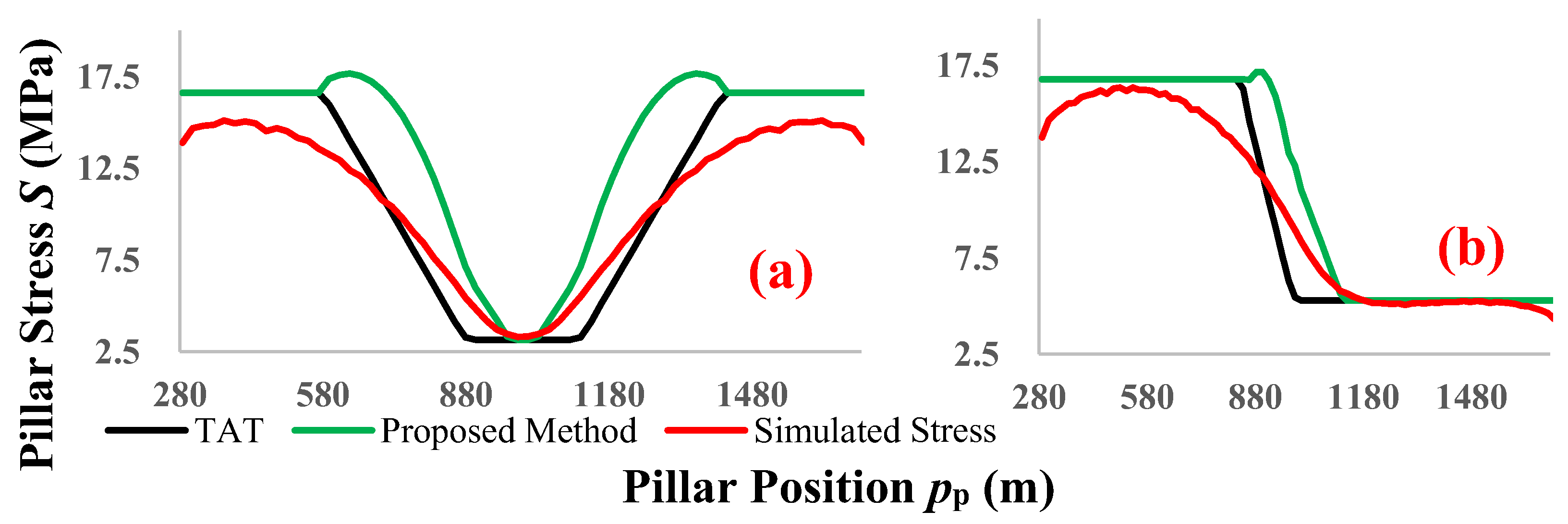
(b) $L_{\mathrm{v}}$ is small and Sections C and C’ intersected. Equations (19) and (20) are still applicable because they are constructed by considering extreme mining conditions. However, a pillar below section C will be affected by the two slopes. When there exists two $K_i$, the maximum value of the two $K_i$ should be used when correcting the pillar stress.

Figure 16 shows pillar stress examples based on the proposed method. The TAT method will underestimate the pillar stress around the slope toe, while the proposed method provides a relative accurate estimation around the slope toe. However, as the proposed method is conservative, it may overestimate the pillar stresses beneath the slope vertex.

5.4. Summary of Pressure Arch Evolution under Different Terrains

The EPA has been proposed for decades and the pressure arch effect has been considered in pillar design [2,5,10,11,12,13,14,15,24]. For cases where the goaf sizes are not large and the terrain is horizontal (where the heights of EPAs usually cannot reach the ground surface), current pressure arch theory can provide a reasonably reliable stress estimation. However, there are only limited studies for cases where the expansion of EPA is restricted by the overburden thickness and the pressure arch reaches the ground surface. With the height of the EPA increasing with the increasing goaf size [5,24], EPA will finally reach the ground, and the EPA turns into a half-arch and half-beam structure such that the TAT area appears in the goaf center (Figure 12). For such cases, the PAT method underestimates the pillar stress while TAT can provide a more reliable estimation. Yu [15] described this phenomenon as mine size effect and suggested that to use TAT instead of PAT for calculating the pillar stress when the ratio of goaf size to mining depth exceeded three or four. In this paper, the mine size effect is essentially the pressure arch effect when the arch reaches the ground surface. According to Equation (3), the ratio of goaf size to mining depth is the shape of an EPA, whereas the overburden properties in Yu’s simulations can result when the EPA reaches the ground with the ratio of goaf size to mining depth of three. Thus, the fixed ratio of three to the ground surface would dictate whether TAT or PAT should be used.

Although TAT area may appear, EPA can still transfer the overburden load to the mine boundaries (the area marked by black dashed lines in Figure 12b). This half-arch part of an EPA is the key factor to produce the pillar stress concentrations around the slope toes. As the overburden thickness varies for mountainous areas, the EPA evolution is restricted by the terrain and its shape can change drastically. The overburden thickness near the slope bottom is too thin to generate a complete EPA; therefore, an intact EPA (Figure 12b) is further divided into a larger EPA under the slope top and a smaller EPA under the slope bottom by the slope (Figure 12c). The accumulated load from the slope (the area marked by black dashed lines in Figure 12c) cannot be transferred to the boundary (in contrast to a horizontal ground), most of the load is applied to the pillar near the slope toe and only limited load is continuously transferred away. Therefore, the stress concentration depends on the intensity of the EPA distribution instead of a single factor such as slope angle, slope height, etc.

In summary, the full EPA evolution controls the pillar stress distribution in an underground mine. In pillar stress estimation, the overburden thickness controls the generation of the EPA, and the variation of EPA shape when EPA reaches the ground surface should be evaluated.

6. Conclusions

To study the terrain effects on the pillar stress within a mine shaft, 1200 models with single slope surface or valley surface have been constructed and investigated. It is found that the pillars around the slope toe suffered from concentrated stresses, which can be reduced for pillars away from the slope toe. The mechanism of stress concentration under a mountainous terrain is that the variation of overburden thickness disturbs the generation of pressure arch. The applicability of PAT and TAT depends on whether the pressure arch reaches the ground surface. At last, the factors affecting the concentrated stresses were analyzed, and an alternative estimation method for mountainous areas is proposed. The major conclusions include:

(1) There will always be pressure arches above a mine void. The small pressure arches above multiple tunnels will emerge into a large extended pressure arch (EPA). The inaccuracy of stress estimation by TAT in small gobs results from the overburden load transfer that is induced by EPA. When the gob size is large enough and EPA reaches the ground surface, EPA can only transfer the overburden loads near gob boundaries, while TAT will take over the load redistribution for the rest of the overburden.

(2) The existence of a slope or a valley significantly changes the shape of EPA, whereas the shallow depth at the slope bottom enables EPA to reach ground surface, restricting the EPA size and its ability in load transfer, and leads to stress concentrations near the slope toe. The shape variation of EPA is primarily affected by $H_{\mathrm{D}}$, $\alpha$, and $H_{\mathrm{B}}$. A large $H_{\mathrm{B}}$ creates a large EPA, and the stress concentration is relieved because the loads are transferred further and shared by more pillars. A larger $H_{\mathrm{D}}$ or $\alpha$ would enhance the acuteness of EPA variation and make the EPA behave less like an arch and increase the stress concentration.

(3) TAT and PAT methods have limitations addressing pillar stress estimation in mountainous areas as they do not consider the terrain effects on the EPA shape. A pillar stress estimation method is proposed for mountainous areas, where the stress values from TAT method have been modified to include the EPA effect.

It should be noted that the calculated stress is an approximate value that is based on the most unfavorable mining conditions. Also, the models are ideal and do not take discontinuities such as joints or faults into account. Therefore, the method can only be used in initial pillar design for a fast pillar stress estimation, and site-specific numerical simulations are suggested for safety purposes when the initial design is completed.