Comparison of Handheld and Echelle Spectrometer to Assess Copper in Ores by Means of Laser-Induced Breakdown Spectroscopy (LIBS)

Abstract

Its properties make copper one of the world’s most important functional metals. Numerous megatrends are increasing the demand for copper. This requires the prospection and exploration of new deposits, as well as the monitoring of copper quality in the various production steps. A promising technique to perform these tasks is Laser Induced Breakdown Spectroscopy (LIBS). Its unique feature, among others, is the ability to measure on site without sample collection and preparation. In this work, copper-bearing minerals from two different deposits are studied. The first set of field samples come from a volcanogenic massive sulfide (VMS) deposit, the second part from a stratiform sedimentary copper (SSC) deposit. Different approaches are used to analyze the data. First, univariate regression (UVR) is used. However, due to the strong influence of matrix effects, this is not suitable for the quantitative analysis of copper grades. Second, the multivariate method of partial least squares regression (PLSR) is used, which is more suitable for quantification. In addition, the effects of the surrounding matrices on the LIBS data are characterized by principal component analysis (PCA), alternative regression methods to PLSR are tested and the PLSR calibration is validated using field samples.

1. Introduction

Non-ferrous metals (NF metals) are important materials in numerous areas of modern life. NF metals are light and noble metals, such as copper, aluminum and gold [1]. They are used in a wide range of applications, particularly in mechanical and vehicle engineering, the electronics and electrical engineering industries, and in the building industry. They are also a fundamental component of future technologies, such as electric traction engines and thin film photovoltaic. As a result, the demand for NF metals will increase in the future [2]. Various options are available to secure the supply of raw materials. In addition to raw material substitution and the more efficient use of resources in production and application, as well as in recycling, ore mining and thus metal extraction can be optimized [2]. The production of commodity metals comprises two main areas: mining, and thus also the prospection and exploration of deposits; and the metallurgical process of the extracted ores and concentrates.

The prospection and exploration of a potential deposit involves many steps and usually takes years. Numerous methods and techniques are used in locating and exploring new profitable deposits, including: remote sensing, geophysical techniques, mapping, drilling and finally geochemical methods [3]. All these investigations are time-consuming and cost-intensive. In particular, the systematic drilling and sampling as well as their analysis in the laboratory are expensive [3,4]. Alternatives could be investigation methods that can be performed on site by using mobile sensor equipment. Examples of these include mobile X-ray fluorescence analysis (XRF) or laser-induced breakdown spectroscopy (LIBS), which allow to analyze the chemical (elemental) composition in situ [3]. An explored deposit becomes a mine if the ore content and extent, as well as the infrastructure of the deposit, make mining profitable [5]. This is carried out by open pit, underground mining or by leaching. In all cases, the ore is concentrated on site by separating ore minerals and gangue. Subsequently, the metallurgical process of the extracted NF ores and NF concentrates takes place [1,3]. Pretreatment, e.g., by roasting and flotation, is followed by melting processes and further thermal treatments. This is followed by thermal and electrical refining and final processing [1]. This procedure leads to a gradual increase in the level of purity. Monitoring metal concentration before, during and after the production process is essential to ensure the quality of the product. Particular attention is paid to the incoming inspection of the ores. In the NF metals industry, various sensor-based techniques are used for incoming and process control; they provide information on properties and surface characteristics of particles and ores, as well as on chemical and mineral composition [6]. The most commonly used sensor techniques in the NF metals industry include X-ray fluorescence (XRF), X-ray transmission (XRT), near-infra-red (NIR), as well as radiometric, optical and inductive sensors [6,7]. In particular, the use of LIBS would also be feasible for ore or concentrate input control. The method allows on site, real-time analysis. In addition, sample material of all aggregate states can be examined almost without sample preparation and practically non-invasively. In LIBS, laser radiation induces a plasma on the sample surface, which excites the sample material. The elements can be identified from the spectral signature of the resulting emission [8,9]. In contrast to other spectroscopic methods, such as XRF, LIBS can be used to analyze all elements of the periodic table [9]. Thus, LIBS is suitable for the analysis of all NFs metals.

Copper is a superlative NF metal: highest electrical conductivity, highest thermal conductivity, highest ductility and only excelled by silver [10,11]. In addition to these properties, the good ductility, corrosion resistance, antibacterial effect and the possibility of recycling the raw material without loss of quality, make copper one of the world’s most important functional metals [12,13]. The demand for copper is high and will continue to increase in the upcoming years, driven by megatrends such as digitalization, energy and transport transformation [13]. Copper occurs in nature in its native form or in minerals [14,15]. To date, about 630 copper-bearing minerals are known [16]. The copper ores of economic interest include, in addition to native copper, the sulfidic ores chalcocite (Cu₂S) and chalcopyrite (CuFeS₂), and the oxidic ores cuprite and malachite [3,13,14,17,18]. The most important ore for copper production is chalcopyrite due to its frequent occurrence [3]. Copper is mainly extracted by open pit mining, but also by underground mining and leaching [5,13]. However, copper mining has to accept new challenges. Environmental protection, land consumption and social responsibility are essential aspects that must be taken into account in modern mining [3]. At the same time, changes in ore quality are to be expected due to lower ore contents and toxic accompanying elements such as arsenic, mercury and bismuth [13,19]. The mineability of copper deposits has declined worldwide over the last 100 years, as the demand for copper is constantly increasing. Currently, raw material deposits with copper contents of 0.4% are mineable [13]. In order to be able to meet the increasing demand for copper and to replace depleted mines, new deposits are being prospected [3].

Copper mining is currently being carried out at numerous deposits worldwide. The main sources of copper, in addition to porphyritic, hydrothermally induced deposits, include volcanogenic massive sulfide deposits (VMS deposits) and stratiform sedimentary deposits (SSC deposits) [3,13,14,20]. VMS deposits are accumulations of sulfides previously formed by black smokers, i.e., geothermal ocean floor vents exhalating superheated metal containing water, in the deep sea. Besides copper, they are sources of several other metals. They are characterized by a wide distribution and a high quality of their ores. Based on mineralogy, several types can be distinguished. One representative of the VMS deposits is the so-called Cyprus type, which describes important copper deposits on Cyprus [3,12,14]. These are mostly small deposits that have medium contents of copper and zinc. Copper-rich veins are also found beneath the ophiolite-bound basalts. Cyprus was already a mining area and production site for copper in the early Bronze Age [3,21]. At its peak, 17 copper mines were active on Cyprus. Today, only the Skouriotissa mine is still in use. It is one of the largest deposits on the island, with 6 million tons of copper estimated total reserves [3,21]. In this “Cyprus-type” deposit, the copper-bearing minerals occur in various associated rocks, such as gabbros or basalts [12]. The main copper-bearing ore minerals of the SSC deposit are chalcocite, bornite and chalcopyrite. One of the best-known European deposits is the Polish Kupferschiefer (copper schist) in the Lubin district. It belongs to the Zechstein Kupferschiefer formation and is part of the world’s most important copper deposits. About 500.000 tons of copper are extracted from the schist here annually [3,12,22].

The mined sulfide copper ore contains a maximum of 2% copper. It is still processed on site. The resulting copper concentrate already has a copper content of up to 30%. The sulfidic ore concentrates are heated to copper matte (~64% copper), which is then roasted. In the process, sulfuric acid is recovered as a by-product of copper production. In further steps, accompanying elements, such as iron, have to be removed. These components are separated as slag. Through further roasting and heating, blister copper and finally coarse copper is obtained from the copper matte, which has a copper content of up to 98%. After further oxidizing and reducing production steps, the obtained tough-pitch copper (99.5% copper) contains only a few impurities and can be converted into cathode copper by electrolytic refining. At 99.99%, cathode copper is the commercial metal with the highest purity. From this, numerous copper forms are produced, which are finally transferred to end-use products. Other important NF metals are recovered from the anode slime [3,5,16,17].

With regard to exploration and smelting, LIBS can be used to determine the qualitative as well as the quantitative elemental composition of copper-bearing ores and concentrates. In addition to the content of copper in the raw material, the determination of the accompanying elements is also relevant for smelting, since different processes are used for metal extraction from sulfide and oxide ores [5]. By controlling the copper quality in the individual production steps of the cathode copper and of the final products, their quality grade can be assured. In this respect, LIBS is often used for qualitative analysis and classification. The determination of the content of the elements contained in a sample is difficult using LIBS because the method has a limited reproducibility due to the experimental conditions [23]. In addition, the surrounding matrix can exhibit high variability in its composition, resulting in numerous chemical and physical factors affecting in the spectra [23,24]. This poses a challenge on the use of univariate regression (UVR) for content determination. Nevertheless, quantification can be achieved by using multivariate methods that take matrix effects into account [23]. One of the most common multivariate analysis techniques is partial least squares regression (PLSR). Here, in contrast to UVR, the entire spectrum is taken in account for the analysis, reducing the susceptibility of the results to matrix effects [23].

In the present work, on the one hand, the use of LIBS in the exploration of copper deposits by means of a handheld spectrometer was investigated. On the other hand, a stationary LIBS was used for the analysis of copper-bearing ores. Only ground ore and rock samples from a VMS deposit and an SSC deposit were used for this study. For calibration, commercially available chalcopyrite and chalcocite minerals were ground up and blended with basalt and schist rock powders, respectively, at various concentrations. UVR was used to construct calibration graphs of the two studied minerals were obtained in both analyzed rocks. In addition to UVR, PLS regression was used to quantify copper content and PCA was used to investigate matrix effects in geologic samples.

2. Materials and Methods

2.1. Samples and Reference Analysis

A total of 152 samples with different copper contents were analyzed in this work whereof 70 are artificial samples (referred to here as synthetic) and 82 are field samples. One subset of the field samples was taken from the Apliki and Skouriotissa VMS deposit of Cyprus. The other subset was taken from the SSC deposit of Lubin in Poland. The accompanying matrix for a sample is either igneous rock basalt in the case of the VMS deposit or schists in the case of the SSC deposit. All samples were in the form of homogenized ground powders.

Reference analysis for the geological samples from Cyprus was performed by aqua regia digestion followed by ultratrace ICP-MS analysis and by LiBO₂/LiB₄O₇ digestion followed by ICP-OES analysis, respectively. Sample copper concentrations range from 41–10,000 ppm. The samples from Poland were referenced by X-ray fluorescence (XRF). Sample copper concentrations range from 0.8–2.4%. For the LIBS analyses, 3 g of ground powders were pressed into pellets at a pressure of 80 kN (P 40, Herzog Maschinenfabrik, Osnabrück, Germany).

2.2. Geological Overview of Deposits

The sample subset from Poland, where the copper deposits belong to the sediment-hosted stratabound copper desposits originates from Lower Silesia, the central area of the Pre-Sudetic Monocline and the North-Sudetic Basin. They are part of the Zechstein copper schist formation. The copper-bearing minerals occur in separate lithological layers, accompanied by dark gray sandstones in the bottom layer, black schists in the middle and carbonate rocks in the top part. The most important copper minerals of this deposit are chalcocite (Cu₂S), chalcopyrite (CuFeS₂) and bornite (Cu₅FeS₄) [22,25].

The second sample subset, which originates from Cyprus, are sulfide deposits that are part of the volcanogenic massive sulfide deposits. The Cyprus type of this deposit belongs to the Troodos ophiolite complex, whose copper-bearing stockwork is surrounded by basaltic pillow lavas. Besides the dominant minerals chalcopyrite (CuFeS₂), pyrite (FeS₂) and sphalerite ((Zn,Fe)S), secondary copper minerals such as chalcocite (Cu₂S), covelline (CuS) and digenite (Cu₁.₈S) occur [26,27].

2.3. Preparation of Synthetic Samples

Powders of the copper-bearing minerals chalcocite (minerals from the New Cornelia Mine, Ajo, AZ, USA) and chalcopyrite (minerals from Füsseberg near Bierdorf, Siegerland, Germany) were used for the preparation of the synthetic samples. The samples were prepared by standard addition. In this process, the copper-bearing minerals were mixed with the respective accompanying matrix of basalt or schist. The used basalt originate from Cyprus and the used schist sample originates from east of the village of Lehesten in the southeastern Thuringian Forest. The schists are from the Saxothuringian as part of the Variscan Mountains. The formerly marine, clayey sediments were deposited in the Missisippian (Lower Carboniferous, ca. 360 Ma). The weighed samples were homogenized and pressed into pellets at a pressure of 80 kN (TP40, Herzog Maschinenfabrik, Osnabrück, Germany). For one pellet a total of 3 g of sample material was used. Here, two pellets were pressed for each concentration of copper, one in basalt the other in schist. A total of 35 samples were prepared for each mineral, 15 in schist and 20 in basalt.

2.4. LIBS Setup and Measurement Parameters

The samples were analyzed by two different LIBS spectrometers. One LIBS spectrometer is a stationary laboratory benchtop instrument equipped with an Echelle spectrometer (Aryelle Butterfly, LTB, Berlin, Germany). For the study, the samples were positioned on a rotation and linear translation stage for enabling a spiral probing pattern during the measurement. This ensured that each ablation was performed on a fresh surface. Plasma at the sample surface was generated by a focused (f = 50 mm) Nd:YAG laser (Bernoulli LIBS, Litron Lasers, Rugby, England, Great Britain, λ = 1064 nm, E = 80 mJ, repetition rate 10 Hz, pulse duration 7 ns). Using a concave mirror (ME-OPT-0007, Andor Technology, Belfast, Northern Ireland, focal length 52 mm, λ = 200–1100 nm), the emission was collected and focused onto an optical fiber that guides the light to the spectrometer. The spectrometer has two wavelength ranges (UV: 190–330 nm, VIS: 278–769 nm). Both ranges were measured separately with a resolution of 25 pm. An ICCD camera (iStar, AndorTechnology, Belfast, UK) was used for detection. A total of about 200 spectra per sample were recorded in the UV and VIS range. For this purpose, 2000 shots were taken in a spiral on the pellet. For each of the 200 spectra, 10 consecutive single shots were accumulated.

The second LIBS spectrometer is a handheld instrument (Z-300, SciAps, WBN, MA). The plasma is generated by the integrated laser (λ = 1064 nm, E = 7.5 mJ, repetition rate 10 Hz, pulse duration 5 ns). The spectrometer has a wide wavelength range (180–960 nm) with a resolution of 100 pm. In order to amplify the LIBS signal, the measurements are additionally purged with argon gas before the measurement. The measurements were performed using the GeoChemPro app. Each sample probed by a grid of 8 by 8 spots, resulting in 64 spectra for each sample. The sampled area was approximately 1 mm². Each pellet was measured three times to obtain a representative set of spectra of the sample.

2.5. Data Pretreatment

All spectra were prepared for analysis by background correction, standard normal variate-normalization, and final averaging of the data. A top-hat filter was used for the background correction. The structuring element length was 20 data points. This corresponds to a filter width of about 0.26 mm. Following the background correction, a SNV normalization was performed. For this, the mean value of the entire spectrum is subtracted from the spectrum. The difference is divided by the standard deviation of the spectrum. The resulting data were finally averaged to obtain a representative spectrum for each sample.

Linear regression was performed using two specific copper lines (324.75 nm and 327.40 nm). The area of each was obtained by numerical integration with the trapezoidal method. The sum of both peak areas represents the total peak area that is plotted against the copper concentration.

The PLSR was performed with a 10-fold cross-validation. It was performed for the number of components with the lowest estimated prediction error.

Outliers were identified using the robust PCA (ROBPCA) method of Hubert et al. [28]. Robust principal component analysis (ROBPCA) is an alternative to classical principal component analysis (PCA), which is very sensitive to outliers due to the empirical covariance matrix of the data. Robust PCA is designed for fast and robust observation of high dimensional data. It uses projection pursuit techniques in the original data space and projects the observations into a subspace with lower dimensions. Here, robust covariance estimates are made. This allows the identification of outliers in a data set and the classification of the data into four categories. Regular observations and good leverage points, which are classified as belonging to the data set, and orthogonal outliers and bad leverage points, which are designated as outliers. In the algorithm of Hubert et al. a so-called outlier map is generated by plotting the orthogonal distance against the robust score distance. In the resulting four quadrants the different data points are grouped. All data points in quadrants I or II are orthogonal outliers or bad leverage points, and are subsequently removed from the original data set [28].

For the principal component analysis (PCA), all spectra were fed after prior background correction, normalization and averaging.

The procedure for the determination of alternative regression models was analogous. In addition, the outliers were identified using ROBPCA and eliminated before applying the regression models.

The preparation of the data, as well as the analyses were carried out with Matlab (version 2021a, MathWorks, Natick, MA, USA). Origin (OriginLab, Northampton, MA, USA) was used to display the results.

3. Results

In the present work, synthetic and field samples of the copper-bearing minerals chalcopyrite (CuFeS₂) and chalcocite (Cu₂S) were analyzed by LIBS. The analyses were performed on two different LIBS spectrometers. First, the samples were analyzed using a handheld device. It is conceivable that mobile LIBS spectrometers could be used in the exploration and prospection of new potential copper deposits. Second, the analysis was carried out with an Echelle spectrometer. The high-resolution spectrometer could be used, for example, in the process analysis of the incoming copper ores and concentrates in the copper production.

3.1. LIB Spectra

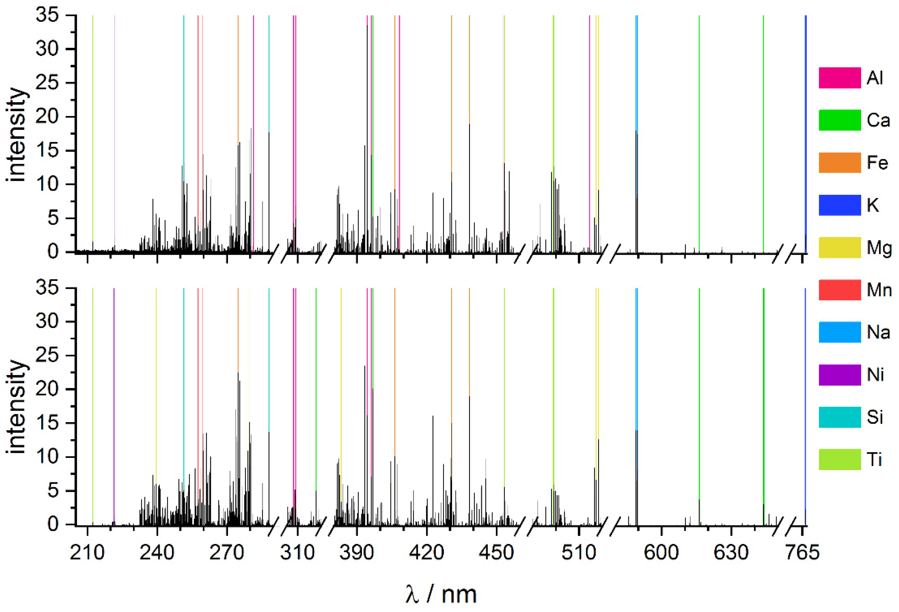
The investigated copper-bearing field samples are from the basalt-related Cyprus-type deposit and from the schist-related SSC deposit from Lubin. A comparison of the obtained LIB spectra (Figure 1) highlights the differences and similarities between the host rocks, basalt and schist. One aim also was to identify the spectral lines of the host rock interfering with the copper lines in univariate regression and to estimate possible matrix effects.

The line-rich LIBS spectra of the host rocks basalt (bottom, Figure 1) and schist (top, Figure 1) show a variety of elements present in both matrices. Differences between the host rocks are mainly in the contents of the individual elements. For example, the mafic minerals of basalt contain high amounts of magnesium and calcium [29]. In contrast, the sedimentary rock of the SSC deposit is clay-bearing and chalky and contains mainly the elements aluminum and silicon [30,31]. In addition, similar contents of manganese are found in both matrices and titanium can be determined in schist. Similar results are also obtained from the reference analysis of the two host rocks (

Table 1. Average contents of the elements in the host rocks basalt and schist from the reference analyses.

Average Element Content/%	Al	Ca	Fe	K	Mg	Mn	Na	Si	Ti
in schist	9.37	0.14	4.65	2.39	1.24	0.08	0.81	29.69	0.58
in basalt	7.07	7.71	2.47	0.77	5.56	0.09	0.90	22.34	0.23

). Furthermore, nickel could be identified in basalt and schist.

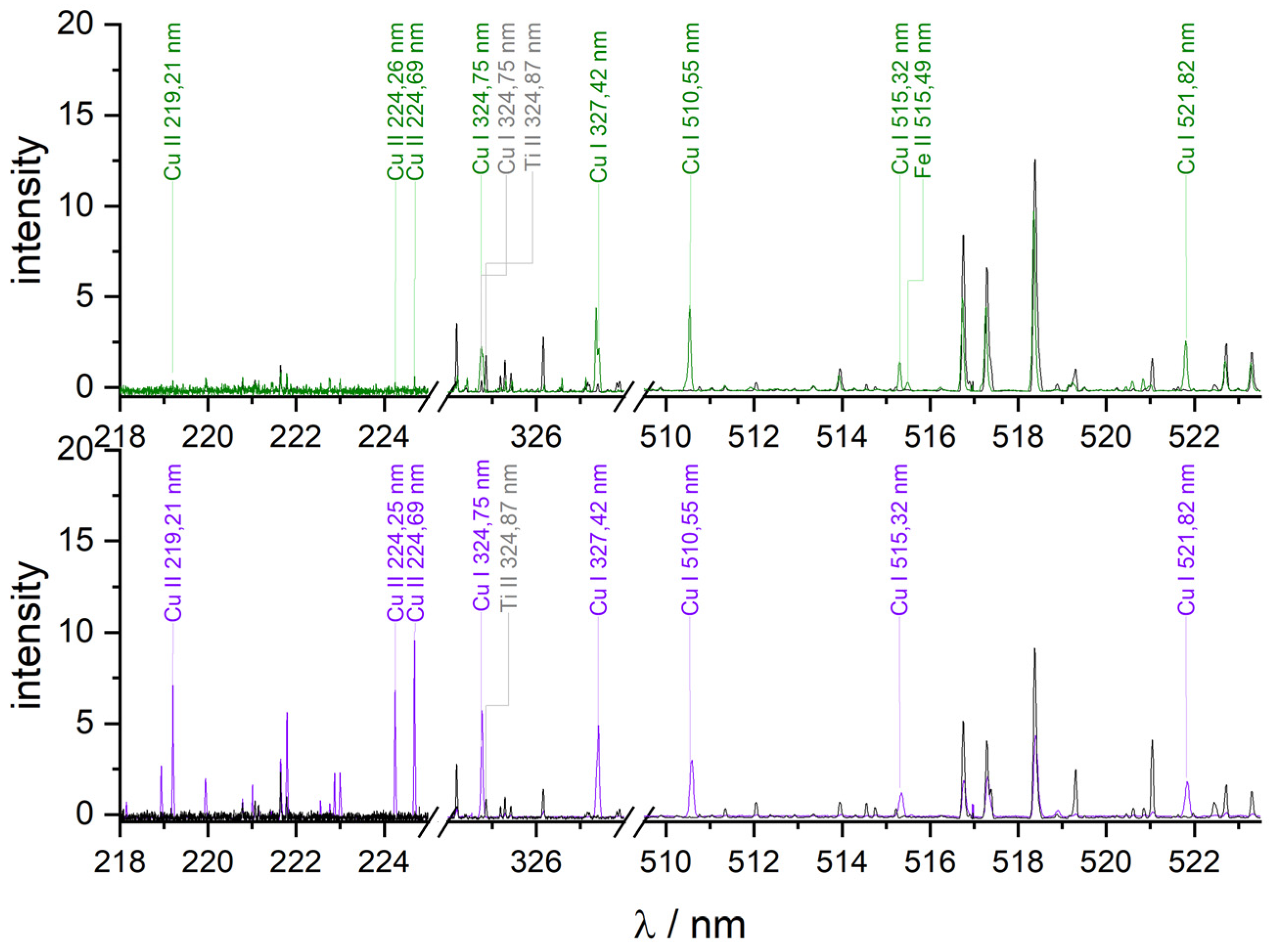
In order to detect possible interferences by the surrounding matrix, the LIBS spectra of the field samples are compared with the spectra of the host rocks with respect to the copper lines (Figure 2).

In basalt, an iron line at 515.43 nm is found in close proximity to the copper line at 515.25 nm. Near to the Cu lines at 324.75 nm and 327.40 nm used in this work, titanium is found in schist and basalt at 324.87 nm. While the accompanying matrix basalt has traces of copper, no copper is found in the host rock schist.

However, since they do not show significant interfering lines, they are well suited as host for the copper minerals in the synthetic samples. The copper lines at 324.75 nm and 327.40 nm are also nearly undisturbed and can be used for univariate regression of the handheld and Echelle spectra.

3.2. Univariate Analysis

One of the most common methods to determine the element contents in different matrices is univariate regression (UVR), in which a calibration function is generated [32]. The calibration function describes a linear or nonlinear relationship between the element content and the area of the element line in the spectrum. Its quality is described by the coefficient of determination R² and the limit of detection (LOD). In the present case, the linear calibration function describes the correlation between the copper concentration and the peak area of the two copper lines at 324.75 nm and 327.40 nm in the spectrum, which could allow quantification of unknown copper concentrations. Other copper lines that could also be used for the analysis, e.g., at 521.82 nm [33], are not sensitive enough due to the low copper concentration in the field samples. This is also clear from the weighting of the spectral lines in the PLSR. In the case of the basalt-containing field samples from Cyprus, the lines at 521.82 nm are not detected. The coefficients of determination and the LOD of the calibration functions which are obtained from the Echelle and handheld spectra are summarized in

Table 2. Coefficients of determination R² and LOD of the univariate regressions of the synthetic samples and the field samples in basalt and schist with the Echelle and handheld spectrometer.

Sample	Basalt		Schist		LIB Spectrometer
	R2	LOD/ppm	R2	LOD/ppm
Cu2S	0.95	140	0.85	1000	Echelle
CuFeS2	0.98	110	0.55	1000	Echelle
Cypriot mines 1 + 2 (basalt)	0.73	110	-	-	Echelle
Polish mine	-	-	0.27	9000	Echelle
Cu2S	0.98	1600	0.41	1000	handheld
CuFeS2	0.96	1100	0.39	1000	handheld
Cypriot mines 1 + 2 (basalt)	0.63	1000	-	-	handheld
Polish mine	-	-	0.31	9000	handheld

.

The LOD are roughly estimated values. With respect to the coefficient of determination three trends can be observed from the results:

• The UVR obtained from the Echelle spectra have higher coefficients of determination than the UVR obtained from the handheld spectra.
• The UVR of the samples in schist (R² = 0.27–0.85) have lower R² than the UVR of the samples containing basalt (R² = 0.63–0.98).
• The synthetic samples (R² > 0.95 in basalt, R² > 0.39 in schist) have UVR with higher coefficients of determination than the corresponding field samples (R² > 0.63 in basalt, R² > 0.27 in schist).

The reasons for the lower linear correlation in the handheld spectra are probably the lower pulse energy, the lower spectrometer resolution and the purging with argon before and during the measurement. Compared to the Echelle spectrometer, where a pulse energy of 80 mJ was used, the handheld spectrometer has only about one tenth of this pulse energy (7.5 mJ). The low pulse energy results in a cooler plasma, which affects the overall line intensity. This change in line intensity can be partly compensated by using argon gas in the sample space. At the same time, the use of a purge gas is associated with uncertainties, since not all ambient air may be completely removed from the sample space. The lower resolution of the handheld spectrometer probably also contributes to the lower linear correlation. Compared to the Echelle spectrometer, which has a spectral resolution of about 25 pm, the handheld spectrometer has a resolution larger than 100 pm. The lower resolution may result in partially overlapping lines. As a result, the exact line position is not known, and line identification becomes difficult. Partial superposition can also lead to errors in the determination of peak areas and thus inaccuracies in the univariate regression, which are reflected in the lower coefficients of determination. The samples in schist show lower R² than those in basalt. The reason could be the material properties of both rocks. Although both rocks are fine-grained and relatively hard, schist has a lower density and is more brittle. This was also observable during measurement. The pellets with a schist matrix were significantly more frequently partially destroyed than the basalt pellets. This destruction of the pellets primarily results in a more uneven surface and a less spatial correspondence between laser focus and surface. This may influence the intensities of the spectra, resulting in lower univariate regression curves.

The univariate regression of the field samples yields lower R² than the synthetic samples. The field samples differ from the synthetic samples in copper content. In addition, they are natural samples that can be more affected by matrix effects because they are exposed to weathering and contamination. This makes the elemental composition of the surrounding matrix more heterogeneous. Interfering spectral lines can occur, which in turn can lead to partial superimpositions and interference of the relevant lines. These result in correlations with lower linearity and thus lower coefficients of determination. Good correlations can only be obtained for the synthetic samples in basalt with the Echelle and handheld spectrometer. For the field samples and especially the samples in schist, the univariate regressions are not suitable as effective calibration functions due to matrix effects. For better quantification, the use of multivariate methods is necessary.

3.3. Multivariate Analysis—Partial Least Squares Regression (PLSR)

As multivariate regression method partial least squares regression (PLSR) was applied. The regression model was validated twice. First, the stratified data set was separated into a training and a validation data set (70:30). The regression model was developed on the basis of the training data and was tested with the validation data. Second, a 10-fold cross-validation of the training data was performed during model development. The coefficient of determination R² and the root mean square error (RMSE) of the validation (R²_V, RMSEV) as well as the cross-validation (R²_CV, RMSECV) were used as figure of merit. 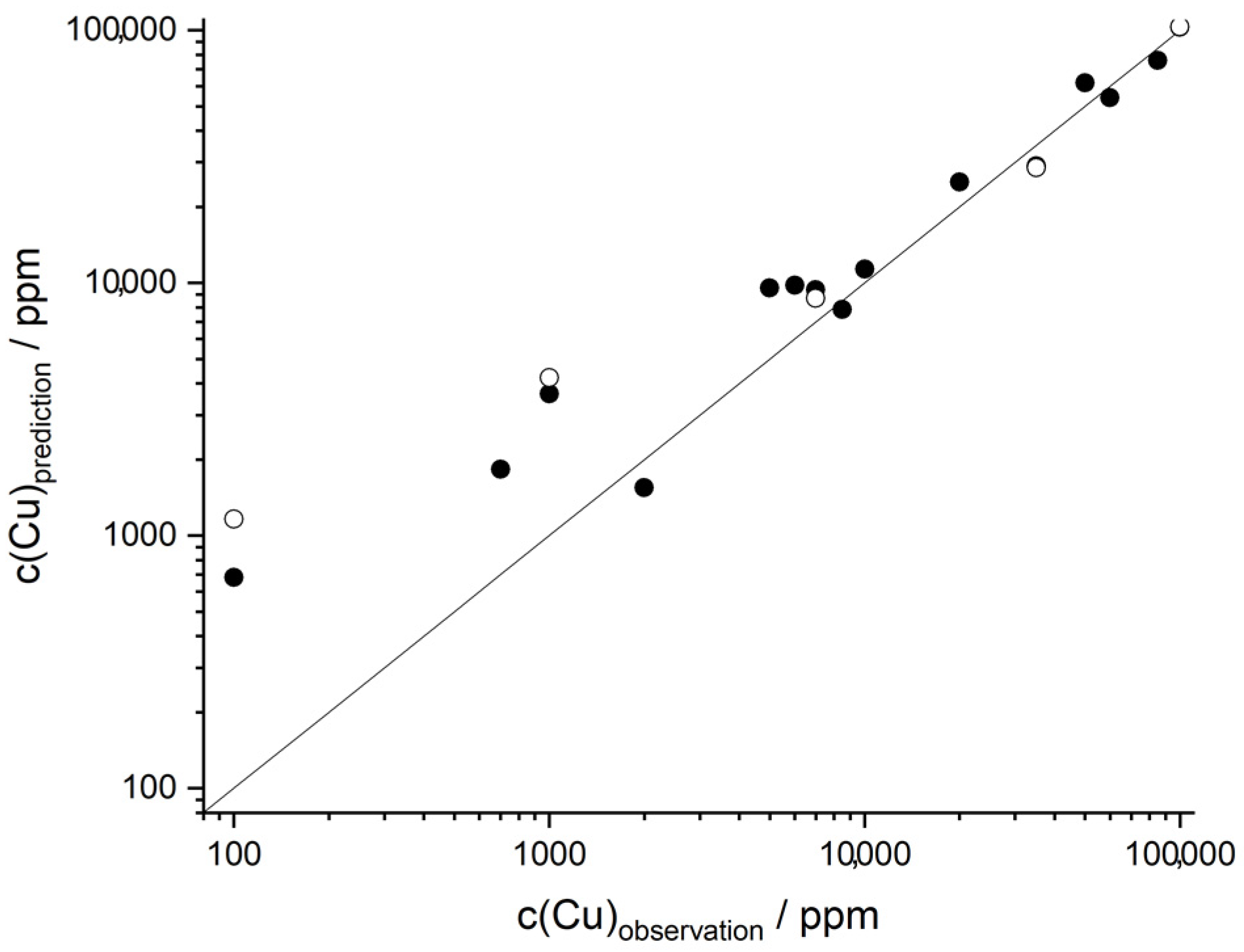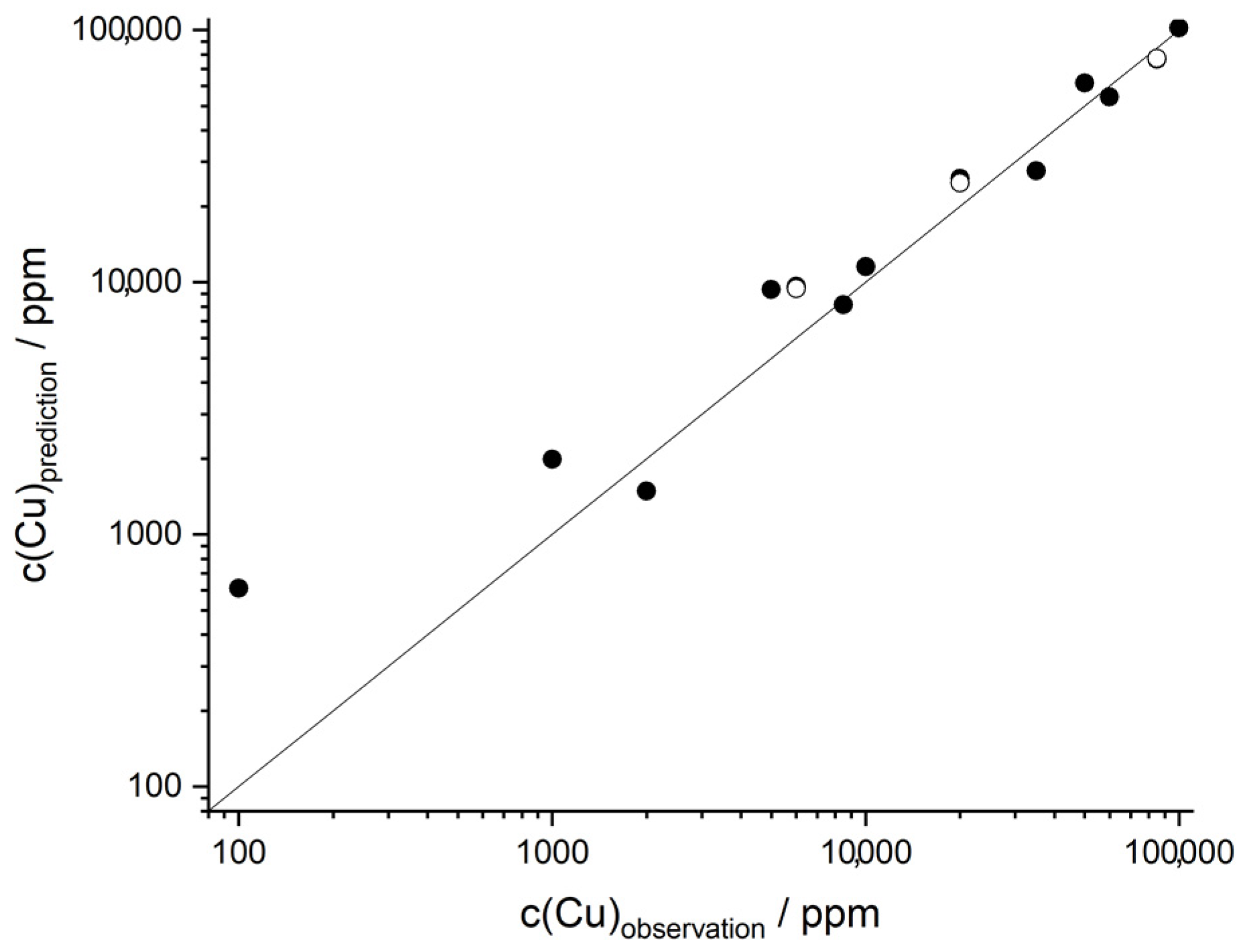Figure 3 shows an example of the correlation plot between observed and fitted response of the PLSR of Cu₂S in basalt from the Echelle spectrometer.

The black dots are the result of the PLS calibration (R²_CV > 0.97), while the circles represent the validation of the model (R²_V > 0.95). Although the validation has a fairly high goodness of fit, the plot shows potential outliers that could negatively affect the correlation. To identify these potential outliers, the robust principal components analysis (ROBPCA) method of Hubert et al. 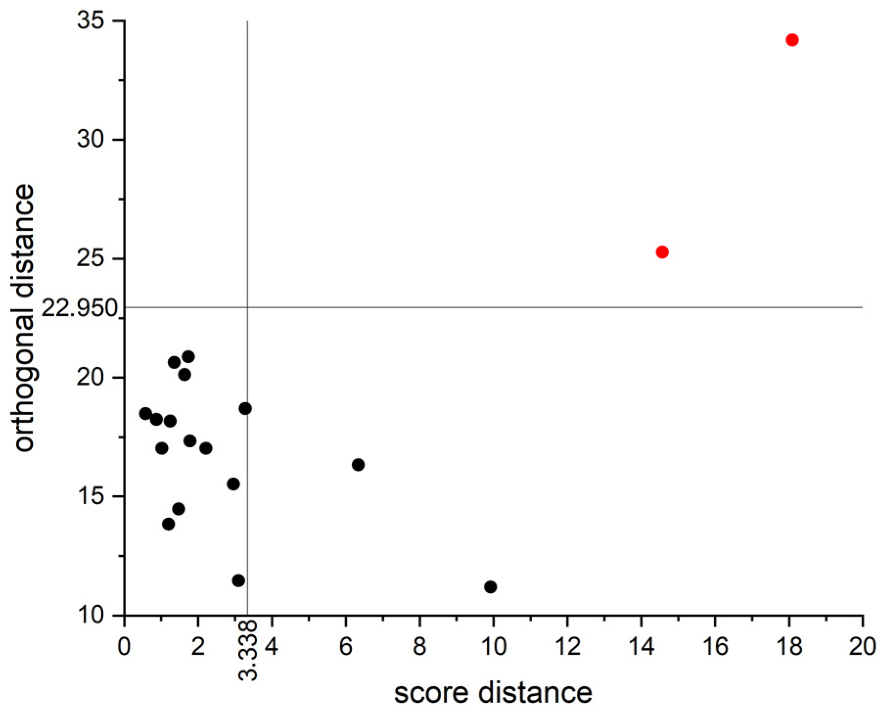is applied [28]. As a result, an outlier map (Figure 4) is obtained, which is plotted between score distance and orthogonal distance.

The first and second quadrants contain the outliers, the so-called bad leverage points and the orthogonal outliers. They are removed from the original data. The remaining data were again divided into a training and validation set. The subsequent PLSR (Figure 5) gives better results in terms of linearity (R²_CV > 0.98) of the calibration model and validation (R²_V > 0.96) after the removal of two data points.

This procedure was applied to all the series of samples studied on the handheld and Echelle spectrometer. The results are summarized in

Table 3. PLSR results of the examined samples in basalt and schist at Handheld and Echelle spectrometer after elimination of outliers by the robust principal components analysis (ROBPCA) method.

Sample	Number of Components	Cross-Validation		Validation
		R2CV	RMSECV	R2V	RMSEV
handheld spectrometer
CuFeS2 in basalt	5	0.74	1.2358	0.61	1.2902
Cu2S in basalt	7	0.96	0.4915	0.92	0.6313
CuFeS2 in schist	5	0.68	1.2229	0.61	1.3138
Cu2S in schist	3	0.58	1.2960	0.60	1.2498
Cypriot mines 1 + 2 (basalt)	6	0.31	1.0249	0.25	1.0303
Polish mine (schist)	4	0.55	2922.8	0.45	3140.6
Echelle spectrometer
CuFeS2 in basalt	4	0.90	0.7628	0.87	0.8154
Cu2S in basalt	5	0.98	0.3454	0.97	0.3449
CuFeS2 in schist	2	0.87	0.8256	0.86	0.7759
Cu2S in schist	2	0.79	0.9538	0.73	1.0026
Cypriot mines 1 + 2 (basalt)	2	0.52	0.8397	0.36	0.9420
Polish mine (schist)	5	0.85	1897.9	0.80	2066.4

. In almost all cases, the elimination of outliers results in a better regression model. The PLSR results of the data measured on the handheld spectrometer show coefficients of determination of R²_CV > 0.55. Exceptions are the sample series of the Cypriot samples (R²_CV > 0.35) and Cu₂S in schist (R²_CV > 0.22). In contrast to the PLSR results of the handheld spectrometer, the PLS regressions of the samples analyzed by the Echelle spectrometer have higher coefficients of determination (R²_CV > 0.85). An exception are again the Cypriot samples with a lower R²_CV > 0.49.

In both cases, Echelle and handheld spectrometers, better regression models are obtained for the synthetic samples than for the field samples, except for the regression of chalcocite in schist. As already mentioned, the synthetic samples have a much smaller variation in the matrix composition than the field samples. The latter ones are inhomogenious, due to grain size variations, and are exposed to natural processes, such as chemical and physical weathering. Due to climate, ground cover, rock properties and the duration of exposure, the surrounding matrices weather very differently [34]. This results in matrices that have a more complex chemical composition, which is dependent on the site of sampling. Rock powders from the same rock were added to the synthetic samples, so that hardly any differences in the matrix can be found. These differences of the rock matrices influence the regressions.

Compared to the UVR, multivariate PLS regression improves the regression models, especially for the synthetic and the field samples in schist measured by the Echelle and handheld spectrometer. For the synthetic samples in basalt, similar regression results are obtained. The UVR of the Cypriot field samples is better than the PLSR.

Wavelength Dependence

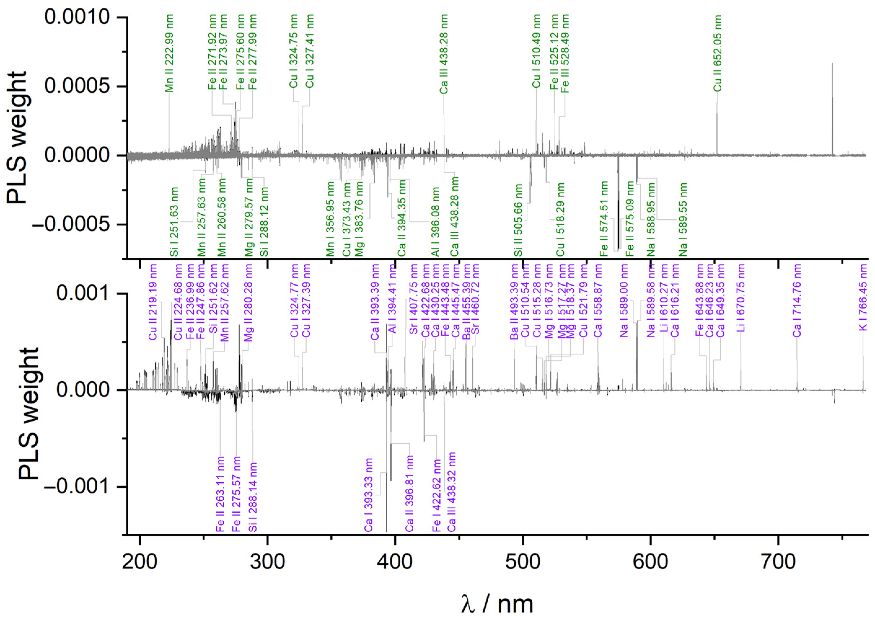
While UVR only considers two spectral lines of the entire spectrum, namely the copper lines at 324.75 nm and 327.40 nm, PLSR includes all spectral lines in the analysis. The PLS weights in Figure 6 show how strong the individual spectral lines of the LIB spectra affect the PLS regression. In this figure, the PLS weights of the first two principal components as a function of the wavelength are displayed for the field samples from Cyprus (top) and Poland (bottom).

In both cases, numerous spectral lines have positive weights. This also includes the two copper lines at 324.75 nm and 327.40 nm, which were used for the univariate regression. In addition to other copper lines of the Cypriot and Polish samples, quite a few lines of the elements of the host rocks basalt and schist can be identified. In the upper spectrum of Figure 6, mainly copper lines and iron lines are found with positive weights. In particular, the copper lines originate from the copper-bearing minerals chalcopyrite and chalcocite. The iron lines may result from the mineral chalcopyrite (CuFeS₂) and the matrix basalt (Cf. Table 1). The negative weighs originate from the accompanying matrix basalt. These include element lines from silicon, magnesium, manganese, aluminum, calcium and sodium. A different picture emerges when looking at the weighting of the wavelengths for the Polish samples (Figure 6 below). In addition to numerous copper lines, many lines with positive weights can be identified that are part of the schist matrix. As in the case of the Cypriot samples, the Cu lines originate from the minerals chalcopyrite and chalcocite. In contrast to the Cypriot samples, significantly more Cu lines can be found here, because the copper contents of the Polish samples are significantly higher than those of the samples from Cyprus. In addition to the copper lines, lines of Ca, Mg, as well as Ba, Na and Li have positive weights. These are part of the schist matrix. Mainly iron lines, but also Ca lines, have negative weights. While calcium is part of the accompanying matrix schist, iron lines may originate from the copper mineral chalcopyrite and the matrix.

Figure 6. Weighting of PLSR as a function of wavelength for PLSR of field samples from Cyprus (top, green) and Poland (bottom, purple) with 2 components each (first component black, second component grey).

Figure 6. Weighting of PLSR as a function of wavelength for PLSR of field samples from Cyprus (top, green) and Poland (bottom, purple) with 2 components each (first component black, second component grey).

3.4. Principal Component Analysis (PCA)

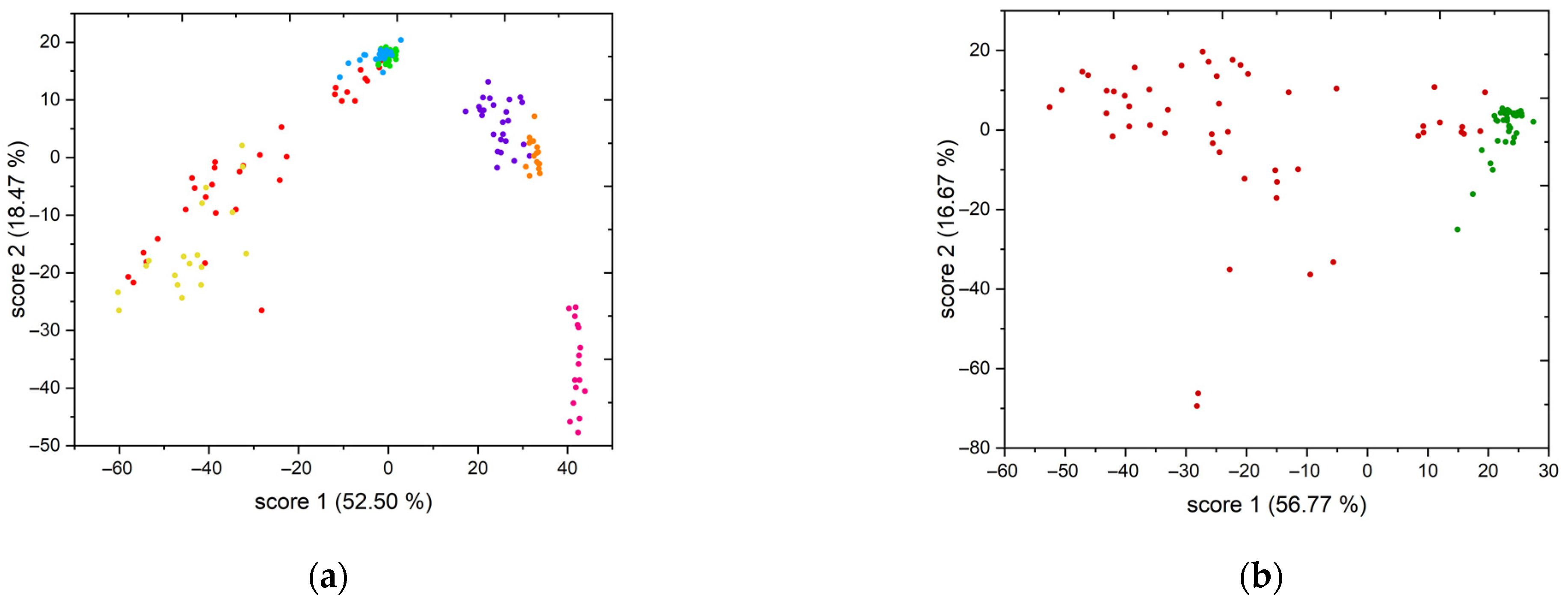
One way to investigate the matrix influence is clustering by the principal component analysis (PCA). For this purpose, all samples examined with LIBS are characterized by PCA. The score plot shows the first two principal components that explain most of the variance. In the score plot, closely grouped data points indicate low variance in the chemical composition of the matrix, whereas a wide distribution of data points visualizes significant differences in the composition of the matrix.

Figure 7a shows the score plot of the handheld spectrometer. The first two principal components explain about 71% of the variance of the analyzed samples. The samples containing basalt (Cyprian mine 1 (red), Cyprian mine 2 (yellow), Cu₂S (green) and CuFeS₂ (blue) in basalt) are spatially well separated from the samples containing schist (Polish mine (purple), Cu₂S (orange) and CuFeS₂ (pink) in schist). The samples form clusters which are well separated depending on the deposit (field samples) or host rock (synthetic samples) but the clusters of the two Cyprus deposits are poorly separated from each other. Synthetic samples such as the Cu₂S-bearing samples in basalt (green) and schist (orange), as well as the chalcopyrite-bearing samples in basalt (blue), are closely grouped. This indicates small differences in the chemical composition of the matrix and explains their excellent regression fits (Table 3). The samples from the Polish mine (purple) and the synthetic CuFeS₂ samples in schist (pink) represent a slightly larger distribution. The matrices of these samples have larger variances in their chemical composition. This results in slightly weaker correlations in the PLS regression. However, the samples of Cyprus mines 1 (red) and 2 (yellow) have the widest distribution in the score plot, indicating larger differences in the chemical composition of the matrices. This also results in a weak correlation of the PLS regression (Table 3). The reason for the large variations in chemical composition in basalt is probably chemical and physical weathering. Depending on the collection site, the field samples were exposed to atmospheric conditions to varying degrees, which led to the differences in composition. These differences were visible on the specimens macroscopically, especially by color differences, but also inclusions and different grain sizes. They are clearly illustrated by the score plot in Figure 7b. Here, the first two principal components from the Cypriot samples (dark red) and the corresponding synthetic samples in basalt (dark green) are shown. In addition to the two clusters that formed, the wide distribution of data points in the cluster of Cypriot field samples is striking. In contrast, the data points of the samples containing Cu₂S and CuFeS₂ in basalt have a rather narrow distribution, illustrating a high similarity of chemical composition, which in turn can be found in the PLS regression, indicated by a rather high coefficient of determination (R²_CV > 0.74. Table 3).

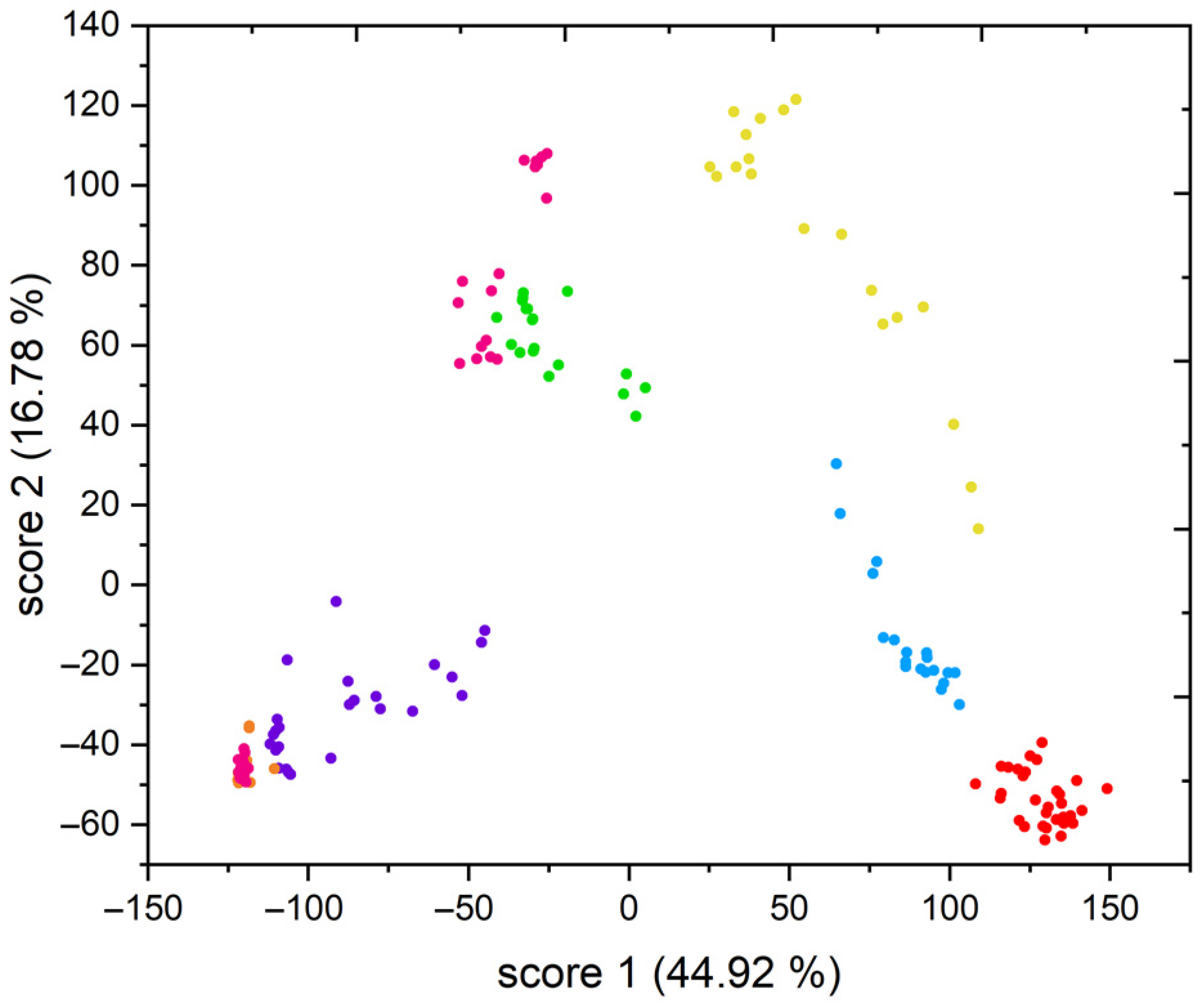
The PCA of the samples analyzed by the Echelle spectrometer yields a better cluster separation of the different sources (Figure 8). Similar to the score plot of the handheld spectrometer, the basalt containing samples (Cyprian mine 1 (red), Cyprian mine 2 (yellow), Cu₂S (green) and CuFeS₂ (blue) in basalt) are spatially separated from the schist containing samples (Polish mine (purple), Cu₂S (orange) and CuFeS₂ (pink) in schist). The clusters are more clearly separated from each other than in Figure 7a, which is also reflected in the coefficients of determination (R²_CV > 0.79) of the PLS regressions (Table 3). At the same time, the data points are more widely separated in the clusters. The regressions of the samples analyzed on the Echelle spectrometer have higher coefficients of determination than those of the samples measured on the handheld spectrometer. The score plot of the samples measured on the Echelle spectrometer mainly shows better separated clusters and more evenly distributed data points.

3.5. Alternative Regression Models

The PLS regression has become a standard tool of chemometrics in chemistry and engineering [35]. In this paragraph, other regression methods are also investigated. For this purpose, the samples were examined by three additional regression methods and different kernel functions. Besides the linear methods principal component regression (PCR) and linear support vector machine (SVM) regression, nonlinear methods such as the quadratic and the cubic SVM, as well as Gaussian process regression (GPR) were examined. As kernel functions, the rational quadratic GPR, exponential GPR and matern 5/2 GPR were used. Using the field samples from Poland measured on the Echelle spectrometer as an example, the results are shown in

Table 4. Different regression models with coefficients of determination (R²) and root mean square error (RMSE) of the regression and validation using the field samples from Poland measured on the Echelle spectrometer after the elimination of outliers by the ROBPCA method.

Model	Cross-Validation		Validation
	R2CV	RMSECV	R2V	RMSEV
PLS regression	0.85	1897.9	0.80	2066.4
PCR	0.73	2636.0	0.69	2943.1
linear SVM	0.71	2744.8	0.65	3161.1
quadratic SVM	0.67	2920.8	0.68	3023.5
cubic SVM	0.62	3125.1	0.74	2714.9
rational quadratic GPR	0.73	2646.3	0.59	3395.1
exponential GPR	0.76	2469.4	0.58	3420.7
matern 5/2 GPR	0.74	2564.8	0.59	3387.1

.

Table 4 shows that there are models which are able to describe the investigated data well, e.g., the linear regression (R²_CV = 0.73. R²_V = 0.69), nevertheless none of the shown models is able to describe the data as accurately as the PLS regression (R²_CV = 0.85, R²_V = 0.80). All other models achieve lower coefficients of determination. This is the reason for applying PLS regression as the method of choice in this work.

3.6. Validation of the PLSR Calibration Based on the Field Samples

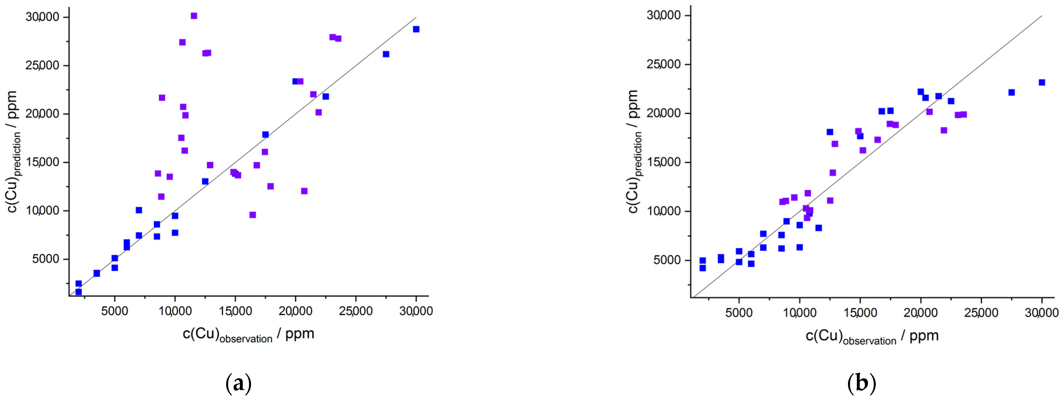
In the exploration of copper deposits many samples have to be measured and only a few samples can be drawn for a later investigation by laboratory-based methods (e.g., ICP-OES). This limited sample volume often results from limited transport capacity and the high cost of reference analysis. The prerequisite for on site measurements in the field is a reliable calibration model. One way of creating this is based on the standard addition method, in which various amounts of the copper mineral are added to a representative host rock. However, since the host rock often varies greatly in its chemical composition in the field, strong deviations in the LIBS signal are to be expected. This is reflected in the PCA score plot, where the clusters of synthetic and real samples are clearly separated and differ in their area. One way of adjusting the calibration function to the field conditions can be the addition of some real samples, which have been characterized (labeled) by reference analysis, to the calibration model. A way to validate the calibration is to apply the obtained calibration model to the field samples. Besides validation, this also shows if and how comprehensive the calibration can be. Additionally, an idea of the predictions on the basis on the PLSR calibration models for other samples with similar associated rocks is gained.

The PLSR calibration models of the synthetic samples of Cu₂S and CuFeS₂ in basalt and schist, respectively, were applied to the Cypriot and Polish field samples (all measured on the Echelle and handheld spectrometers, respectively) for this purpose.

Figure 9a shows the result of the PLSR calibration of the synthetic samples of Cu₂S and CuFeS₂ in schist (dark blue) and the validation with the Polish field samples (purple). The validation only achieves a coefficient of determination of R² = −1.95. Thus, the PLSR calibration of the synthetic samples in schist is not suitable to quantitatively predict element contents of the Polish field samples. To increase the prediction accuracy, data from the field samples were successively added to the synthetic samples and the calibration and validation were performed again. The best result was obtained after adding 22% randomly chosen field samples to the calibration model of the synthetic samples (Figure 9b). A coefficient of determination of the validation of R² = 0.79 could be obtained (

Table 5. Validation results (R², RMSE) of PLSR of the synthetic samples in schist validated with the Polish field samples.

Samples		Spectrometer	Components	Validation
Training Data	Validation Data			R2V	RMSEV
syn. samples in schist incl. ~22% polish field samples	Polish field samples	Echelle	4	0.79	2180.3
syn. samples in schist incl. 40.5% polish field samples	Polish field samples	handheld	4	0.42	3560.4

).

Thus, this calibration method is suitable to quantitatively predict element contents in unknown field samples. The corresponding investigations of the field samples obtained by the handheld instrument and from the Cypriot field samples are not successful. This could be expected because the corresponding figures of merit of regression (Table 3) are poor but in principle similar relative trends are obtained.

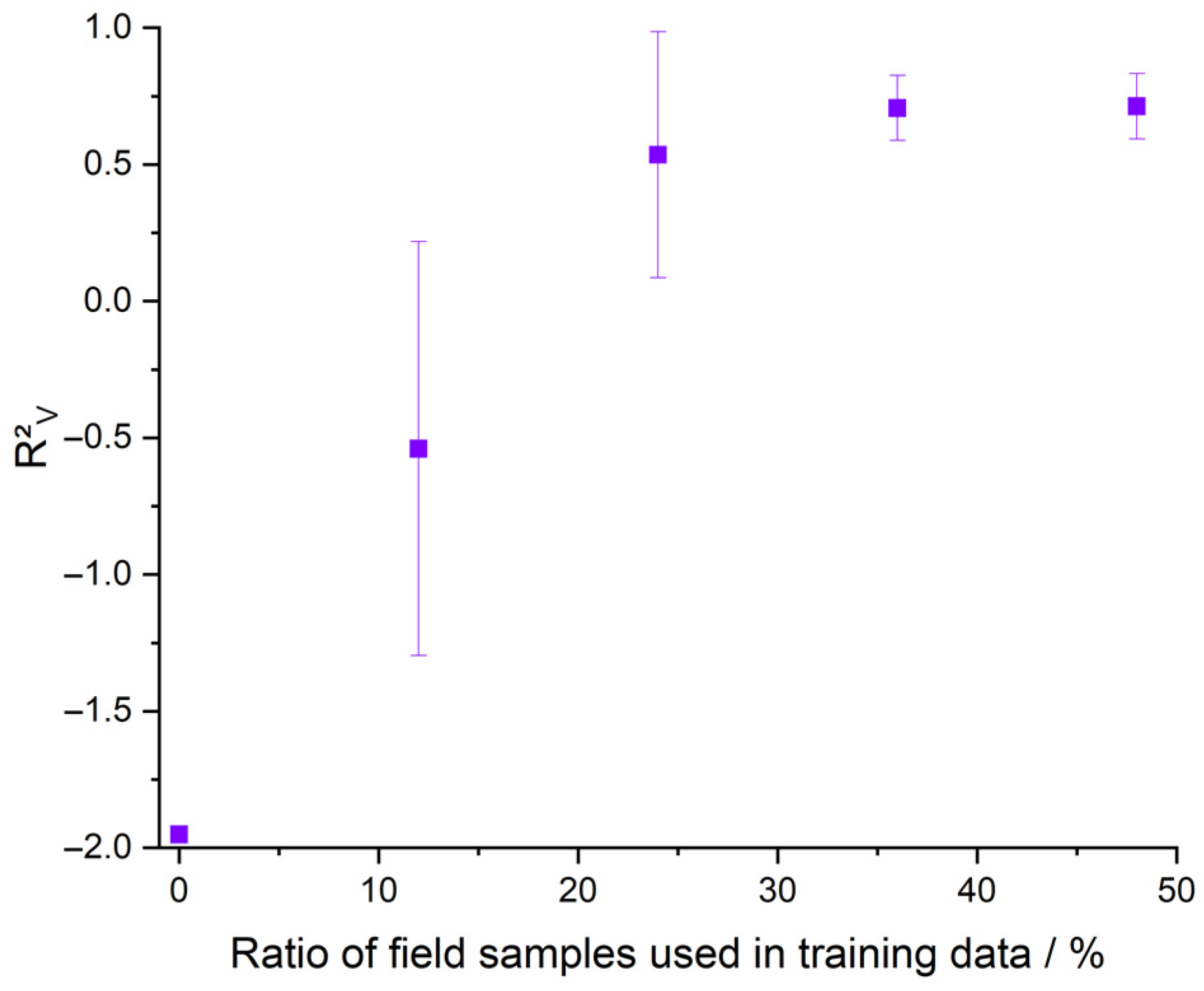
In contrast to the Polish samples (c(Cu) = 0.8–2.4%), the Cypriot samples (c(Cu) = 41–10,000 ppm) possess a much lower concentration of copper. This seems to be the reason for the weaker correlation of the data. The necessary addition of the field samples to the training data shows that the matrix effects of the field samples influence the calibration. Since the complex chemical composition of the field samples cannot be represented in the synthetic samples, the addition of some field samples to the calibration data is a reasonable way.

Figure 10 shows the evolution of the R²_V of the validation data with increasing ratio of field samples to the synthetic samples up to a ratio of about 50%.

If this ratio increases, the coefficients of determination also increase and converge to a plateau at almost 22% of the field samples added to the synthetic data. In the case of the data measured on the Echelle spectrometer, the coefficient of determination reaches a value of R² = 0.79 at an admixture of 22% and of R² = 0.81 at an admixture of 50%. Especially with regard to the application during prospecting and exploration work, the use of a smaller field sample data set is reasonable, since a smaller part of field samples has to be taken and analyzed in the laboratory. This can save time, resources and costs and still achieve good results.

4. Summary and Conclusions

LIBS is a promising method for the detection and quantification of copper in copper-bearing samples, as this technique can rapidly determine numerous elements simultaneously in a matrix with little or no sample preparation. LIBS is compromised by its strong matrix dependence. This requires careful calibration and the use of multivariate methods. The handheld instrument used in this work is particularly suited for use in the field. The semiquantitative investigations allow an orientation in the field. In addition to the mobility offered by this handheld instrument, the simplicity of use, purging with argon, and measurements in a grid are advantageous for field studies. In contrast, the stationary LIBS system with an Echelle-based detector offers a higher spectral resolution and a larger excitation energy, which also allow a more accurate view of the samples in terms of multivariate analysis of the spectra.

In the present work, two data evaluation methods are used to quantify the copper contents in the studied ores. The first approach is a calibration using synthetic samples in conjunction with univariate evaluation. Here, the peak areas of the copper peaks at 324.75 nm and 327.40 nm were used for the analysis. However, due to strong matrix effects, the obtained univariate regressions are in the most cases not suitable as calibration functions. Exceptions are the regressions of the Cypriot field samples measured with Echelle and handheld spectrometer. In a second approach, the multivariate method of PLS regression, after an elimination of outliers using ROBPCA, is used. This resulted in better calibration models. PCA was performed to estimate the matrix effects. Applying alternative regression models to the LIBS data did not improve predictions compared to PLSR. Finally, the predictive power of the PLSR was tested. For this purpose, the regressions of the synthetic samples were applied to the field samples. It turns out to be advantageous if the training data set already contains some labeled field samples. The use of a mobile LIBS spectrometer that can be deployed in the field can save on sampling, transportation and analysis costs when prospecting and exploring for new copper deposits. At the same time, the use of a high-resolution LIBS spectrometer allows more accurate determination and monitoring of copper grades, e.g., during the refining and production process for high-purity copper.

In the future, this work should be supplemented by field samples from additional copper deposits, especially with regard to other host rocks. In addition, the samples could be expanded to include copper concentrates of different processing stages.