An Improved Python-Based Image Processing Algorithm for Flotation Foam Analysis

Abstract

For industrial flotation foam image processing, accurate bubble size measurement and feature extraction are very important to optimize the flotation process and to improve the recovery of mineral resources. This paper presents an improved algorithm to investigate mineral flotation foam image segmentation for mineral processing. Several libraries implemented for the Python programming language are used for image enhancement and compensation, quantitative analysis of factors influencing the image segmentation accuracy, and suggestions for improvement of the flotation foam image processing. The bubble characteristics-size and morphology-and the influence of the flotation conditions on the flotation foam image are analyzed. A Python implementation of the Retinex image compensation method-region-adaptive and multiscale-is proposed to address known issues of uneven illumination and shadows affecting flotation foam images, thereby improving brightness uniformity. Finally, an improved version of the watershed segmentation algorithm included in the Python Open Source Computer Vision library is used for segmentation analysis. The accuracy of the flotation foam image segmentation is 3.3% higher than for the standard watershed algorithm and the segmentation time is 9.9% shorter.

1. Introduction

Mineral resources are extremely important for human development. They represent critical materials for the industry, and they ensure security, economic growth and self-sufficiency for a country. China has a long history of mineral resource exploitation. The mineral industry has not only accelerated the Chinese urbanization process, but it has also allowed for the coordinated development of Chinese regions and has been fundamental for employment and social stability [1]. Mineral resources are non-renewable Because of increasing consumption and intensive exploitation of larger, more accessible deposits, new extraction methods focus on smaller deposits of finer, lower-grade ore. Concurrently, extraction efficiency is constantly improved to increase the quantity of available mineral resources. Mineral flotation is the most widely used technology in the mineral processing industry. It was developed in the late 19th Century and gradually applied to industrial production in the early 20th Century. Since then, flotation equipment and technology have been investigated and regularly improved [2].

Currently, more than half of the non-ferrous metal ore is extracted using froth flotation processes. Froth flotation is a method of mineral separation that differentiates minerals by their surface physical and chemical properties. Despite extensive worldwide research on flotation processes, there is currently no mathematical model to characterize such processes accurately or to optimize flotation control [3].

In China, current flotation processing sites rely on human observation to determine the state of the flotation foam and to adjust the dosage and ventilation volume. This method is not appropriate to meet the current demand in mineral separation for social and economic development [4] and to comply with current requirements of energy saving and emission reduction for climate change mitigation. Surface characteristics of flotation foams strongly depend on the flotation conditions and can be used as indicators. Automating the analysis by replacing human observation and combining data acquisition, processing, and display into a single computer operation would greatly simplify the extraction process [5]. Flotation process parameters can be characterized more clearly from the visual features of a computer-generated foam image. These results can then be used to build a prediction and monitoring model of the flotation system, in order to achieve flotation process control and real-time detection, thereby improving flotation efficiency and reducing errors caused by manual observation [6]. Indeed, although experienced operators can infer the flotation system operation status from the foam, more subtle structural changes in the foam cannot be diagnosed manually. Therefore, stability detection and real-time regulation of the flotation system are difficult to achieve [7,8].

Since the late 20th Century, extensive research has been conducted worldwide to replace manual monitoring with machine vision. The European Union—within the European Strategic Programme on Research in Information Technology/Long Term Research framework—launched the “Machine Vision-based Bubble Structure and Color Representation” project, involving several universities and companies in Finland and Sweden [9,10]. Wang et al. [11] proposed using valley edge detection and tracking to segment foam images. High-illumination points were used to define illumination thresholds for foam bubble classification, then valley bottom edges were tracked in four directions [11]. Citir et al. proposed a two-iteration method for bottom edge tracking, first using pixel minima to mark local regions, then applying the results to refine the edges [12]. Sadr-Kazemi and Cilliters [13] applied the morphological watershed method to flotation foam segmentation. Their robust method used histogram equalization and the “marker” concept—the maxima within the foam bright spots become the identifiers [13]. Bonifazi et al. also applied the watershed method to flotation foam segmentation analysis [5]. Forbes postulated that the combination of texture feature analysis and the watershed method could improve segmentation accuracy [14]. Zhang et al. proposed a watershed segmentation algorithm based on optimal labeling for bubble size measurement [15]. Lezoray et al. proposed an unsupervised clustering classification and region-merging method for color image segmentation, which achieved good results [16].

Despite extensive research, the high accuracy of foam image processing is difficult to achieve for all working conditions and in complex environments [17]. Therefore, the complexity and specificities of flotation foam must be studied. Accurate measurements of the flotation foam bubble size are especially important [18]. Recently, the industrial technology for machine vision monitoring and control has become largely automated. To fully exploit limited mineral resources—such as lean ore or refractory mineral dressing—and to improve their recovery and utilization rates, technologies using machine vision must be applied to mineral flotation detection.

This paper presents an in-depth analysis of flotation foam generation mechanisms and of the correlation between bubble size and working conditions. To improve the characterization—size and morphology—of foam bubbles and the measurement accuracy, the paper defines several methods to evaluate flotation foam image properties—clarity, illumination uniformity, and multiscale enhancement. Furthermore, an adaptive foam image segmentation method is proposed for parameter measurement. Finally, segmentation accuracy and efficiency are assessed to improve the accuracy and robustness of the flotation foam segmentation algorithm [19].

2. Error Analysis and Characterization of Flotation Foam Images

The flotation process is the separation of minerals from finely ground ore at a liquid–gas interface. The foam bubble properties—structure, stability, size, shape and number—all affect mineral flotation. For example, even if the ore selection conditions are suitable for flotation, improper adjustment of the foam bubble shape might negatively influence flotation. Flotation foam characteristics are adjusted by modifying the physical and chemical conditions during the flotation process.

2.1. Factors Influencing the Flotation Foam

The characteristics of mineral flotation foam depend mainly on the flotation agent, the pulp concentration, the mineral particle size, the wind pressure, the foam layer thickness and the work environment. For example, the lighting conditions in a milling plant influence the flotation conditions. Furthermore, industrial flotation is a mechanized process that generates noise, with a possible effect on the flotation image bubble extraction accuracy [20]. Therefore, flotation foam image denoising is an important step of the flotation process.

The qualitative relationship between the flotation operation variables and the foam bubble morphology is shown in

Table 1. Relationship between flotation operation variables and foam bubble morphology.

Operation Variable Description	Bubble Characteristics
The amount of foaming agent is large	Bubbles are small and bubbles are stable
Small amount of foaming agent	Bubbles are large and bubbles are unstable
The more inhibitor	The bubbles are small and round, and the foam load is small
The less inhibitor	Bubbles are large, elliptic, sticky and slow moving
The pH value of the pulp increases	Bubble increase
The pH value of the pulp decreases	Bubble decreases
High pulp concentration	The bubbles are large, elliptic, slow moving and high bearing rate
Low pulp concentration	The bubbles are small, round and unstable
Air pressure is high	The bubbles are large, elliptic, fast and low mineralization
Air pressure is down	Bubbles are small, round, slow and highly mineralization

.

2.2. Compensation of Machine Vision Errors during the Flotation Process

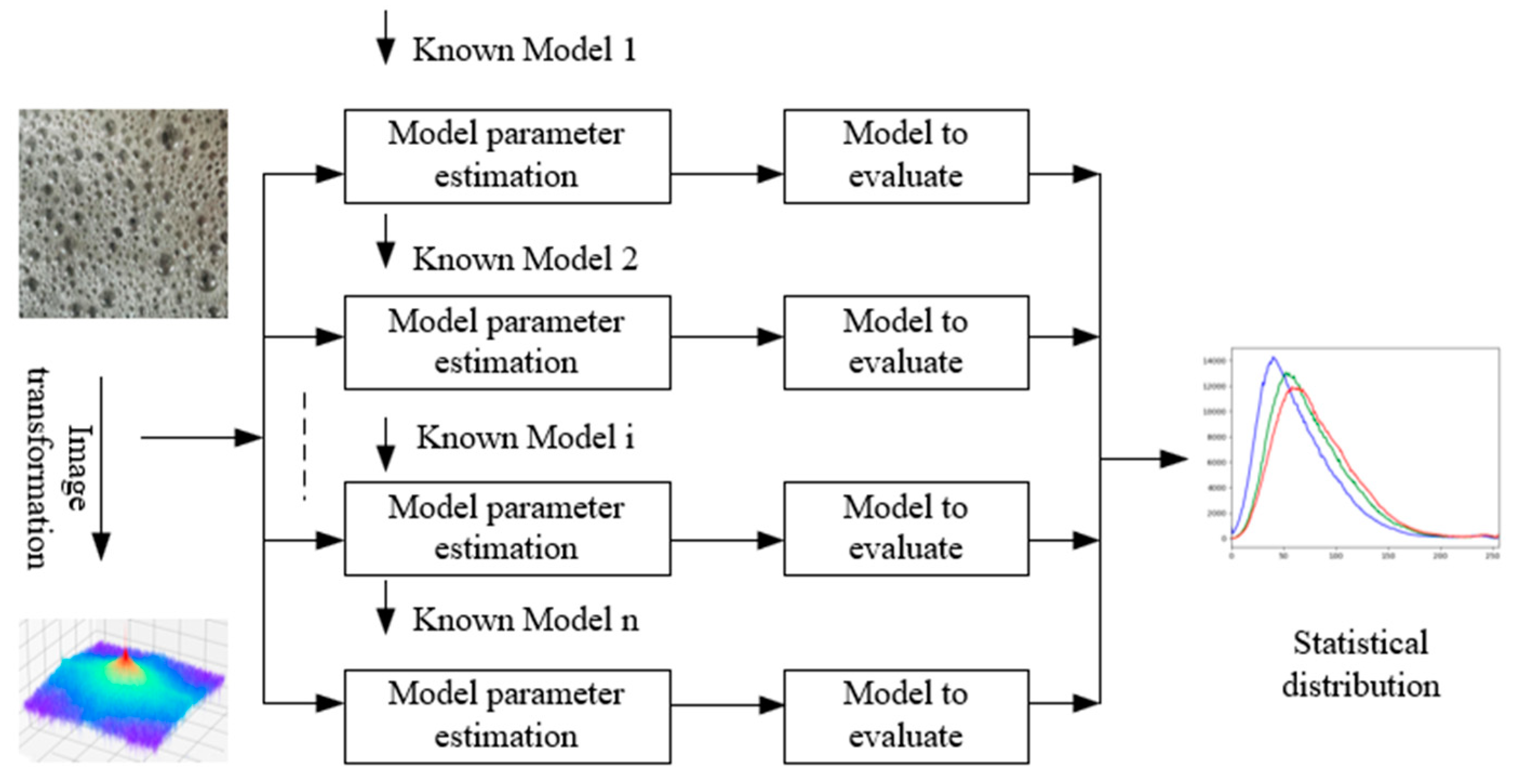
2.2.1. Model Definition for Machine Vision Image Recognition

Statistical modeling provides new possibilities for automatic detection, measurement, analysis and identification of flotation foam images with the random accumulation of mineralized bubbles at the surface. Currently, most statistical image models use parameter quantization methods, because they are simple to implement and easy to understand [21,22]. A schematic representation of statistical image modeling by parameter quantization is shown in Figure 1.

During the statistical image modeling process, a specific mathematical image transformation is applied to the original image pixels. The statistical pixel distribution analysis is then performed in the transform domain. The most common image transformation operators for industrial mineral processing are the wavelet transform, the Gabor filter, and high-order Gaussian derivative filter banks. Empirical probability density functions are then used to fit the statistical pixel distribution and characterize the image.

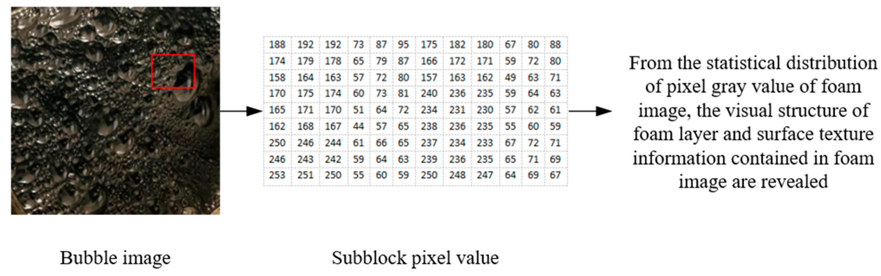
2.2.2. General Principle for Statistical Analysis of Flotation Foam Images

An image, as perceived by the human body, is a form of physical information (light) collected and interpreted by the eye–optical nerve–visual cortex processing system. A digitized (computerized) image, such as the foam image shown in Figure 2, is stored only as a two-dimensional pixel value matrix. Specific information on the image—shapes, granularity—or on the physical process—uneven foam surface, specific flotation conditions—is not included. Therefore, the purpose of machine vision monitoring is to allow the computer to emulate the observation capabilities of the human visual system. If the algorithm is accurate enough to automatically derive surface information from the foam images, flotation control and flotation process operations can be automated.

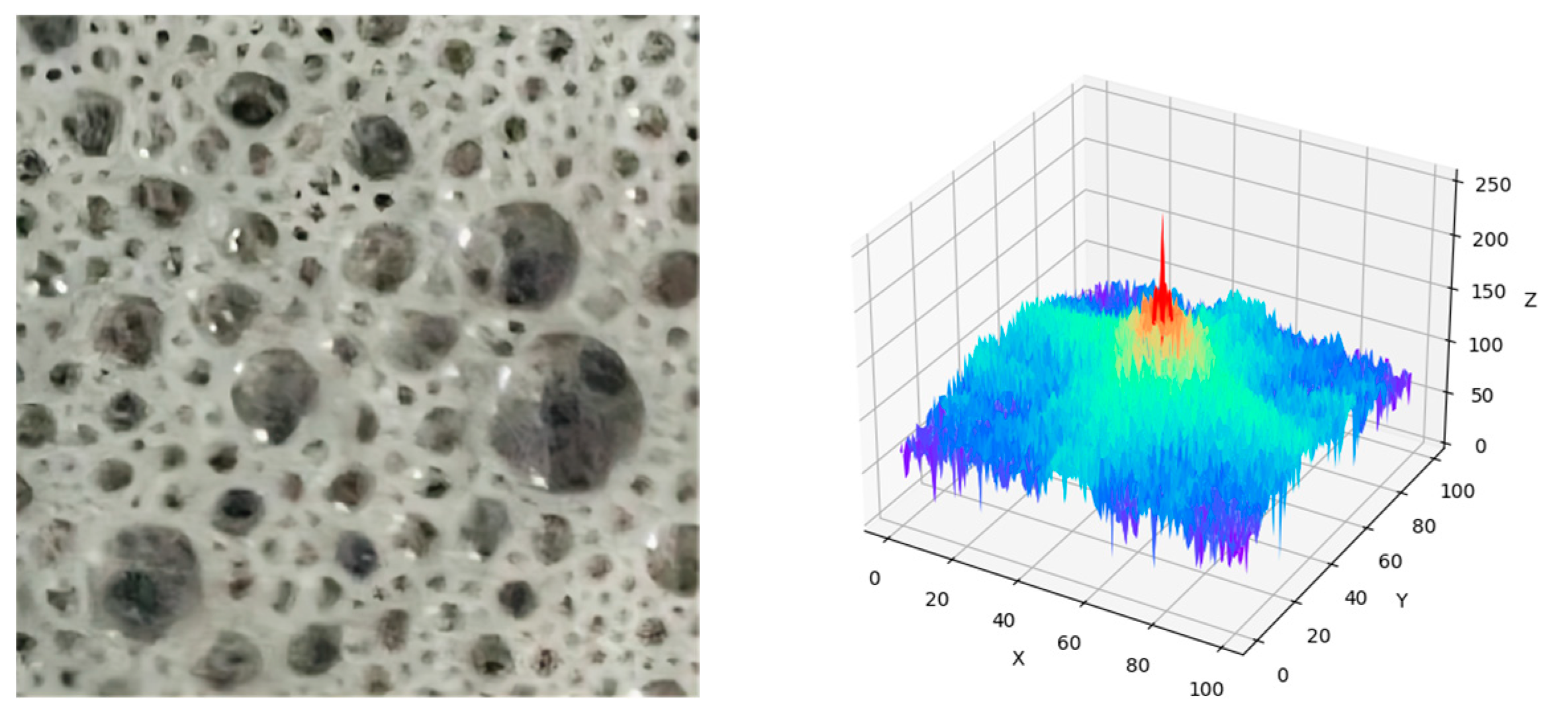
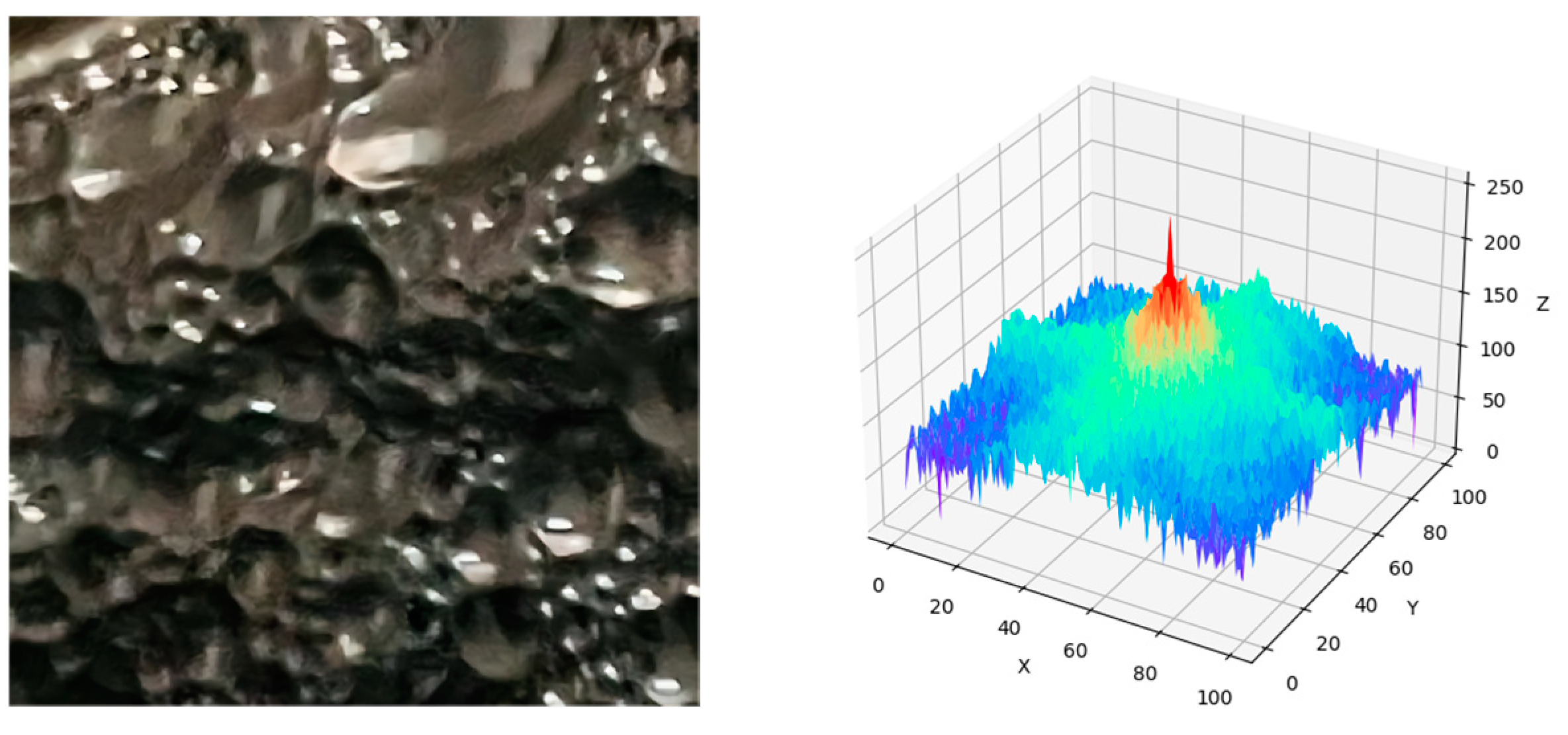
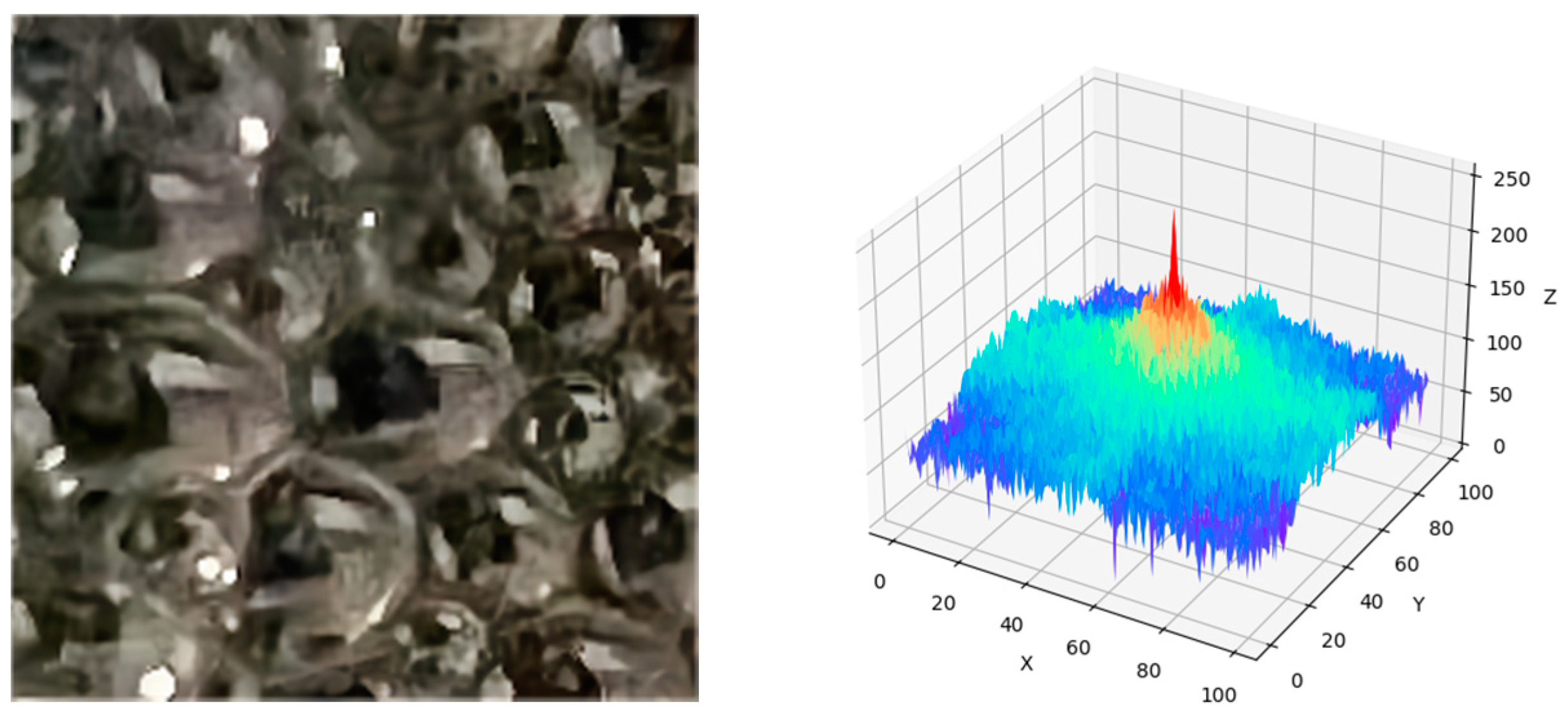
2.2.3. Flotation Foam Image Spectrum Characteristics

For an observation system, the pixels composing a digital image represent discrete point sources. Mathematically, point sources can be represented by the Dirac delta function (or distribution). The two-dimensional delta function δ(x, y) can be expressed as:

$${\displaystyle \underset{x,y}{\iint }\delta (x,y)dxdy=1}$$

(1)

By definition, δ(x, y) = ∞ when x = 0 and y = 0, and its value is zero everywhere else. The δ function is a generalized function over the real numbers. Therefore, for any function f(x, y) that is continuous at a point (x₀, y₀), the function value at that point is expressed as:

$${\displaystyle \underset{x,y}{\iint }f(x,y)\delta (x-x_0,y-y_0)dxdy=f(x_0,y_0)}$$

(2)

Assuming f(x, y) is an analog image, its amplitude f and coordinates x and y must be discretized to convert it into a digital image for computer image processing. This digital image is the matrix form—obtained by sampling and quantization—of the continuous, analog f(x, y). If f(x, y) is sampled on a uniform grid with sampling intervals Δx and Δy in the x direction and y direction, respectively, the coordinates of the sampling points on the image are x = mΔx and y = nΔy, where m and n are signed integers. The sampling function for one point is defined by a δ function. The discrete image sampling function s(x, y) is thus:

$$s(x,y)={\displaystyle \sum _{m=-\infty }^{\infty }{\displaystyle \sum _{n=-\infty }^{\infty }\delta (x-m\Delta x,y-n\Delta y)}}$$

(3)

The sampled image f_s(x, y) is the product of the original simulated image f(x, y) and the sampling function s(x, y):

$$f_s(x,y)=f(x,y)s(x,y)$$

(4)

To obtain the image spectrum, the Fourier transform operator is applied to both sides of Equation (4). We define the Fourier transforms of f(x, y) and s(x, y) as F(u, v) and S(u, v), respectively. Applying the convolution theorem, the Fourier transform of f_S(x, y) is then expressed as:

$$F_s(u,v)=F(u,v)\ast S(u,v)$$

(5)

Equation (5) can be written in its specific integral form as:

$$F_s(u,v)=\frac{1}{\Delta x\Delta y}{\displaystyle \underset{\omega =-\infty }{\overset{\infty }{\int }}{\displaystyle \underset{\omega =-\infty }{\overset{\infty }{\int }}F({\omega }_1,{\omega }_2){\displaystyle \sum _{m=-\infty }^{\infty }{\displaystyle \sum _{n=-\infty }^{\infty }\delta (u-{\omega }_1-m\Delta u,v-{\omega }_2-n\Delta v)d{\omega }_{1}d}}}}{\omega }_2$$

(6)

After calculation, Equation (6) becomes:

$$F_s(u,v)=\frac{1}{\Delta x\Delta y}{\displaystyle \sum _{m=-\infty }^{\infty }{\displaystyle \sum _{n=-\infty }^{\infty }F(}}u-\frac{m}{\Delta x},v-\frac{n}{\Delta y})$$

(7)

Equation (7) shows that the spectrum of the sampled image is composed of the original continuous image spectrum and of an infinite number of periodic translation spectra. Therefore, the spectrum derived from the foam image by Fourier transform gives the energy of all frequencies forming the image. The number of frequencies corresponds to the number of pixels in the spatial domain image.

We consider the following continuous image function:

$$f(x,y)=[3\sin (2\pi n_{1}x+\frac{\pi }{3})+4\cos (2\pi n_{2}x)]\cdot [3\sin (2\pi n_{1}y+\frac{\pi }{3})+4\cos (2\pi n_{2}y)]$$

(8)

The sampled image and the Fourier spectrum of f(x, y) corresponding to scheelite, coal gangue and lead-zinc ore flotation foams for n₁ = 3 and n₂ = 4 are shown in Figure 3, Figure 4 and Figure 5, respectively.

The autocorrelation function of an image characterizes distance and orientation correlations between pairs of image pixels. Thus, the image spectrum is directly related to the autocorrelation function. By examining the spectra in Figure 3, Figure 4 and Figure 5, we conclude that there are correlations between image pixels for each mineral. Therefore, determining the image autocorrelation function would yield information on the image.

We define a foam image I(x, y) and its Fourier transform $\widehat{I}$(ξ, η). The frequency energy spectrum A(f) is equal to |${\widehat{I}}^2$(ξ, η)|, where $f=\sqrt{{\xi }^2+{\eta }^2}$ is the direction of average energy in the frequency domain. The spectrum A and the spatial frequency f are related by:

$$A=b/f^a$$

(9)

This is equivalent, in logarithmic coordinates, to:

$$\log A=\log b-a\log f$$

(10)

Because the image spectrum shows the same energy in each frequency band, the image is scale-invariant.

$$E_{f-2f}={\displaystyle \iint {}_{f^2\le {\xi }^2+{\eta }^2\le {(2f)}^2}}\left|{\hat{I}}^2(\xi ,\eta )\right|d\xi d\eta ={\displaystyle {\int }_f^{2f}2*\pi *x*\frac{const}{x^{a/2}}}dx$$

(11)

Substituting the approximate value of constant a (a = 2) into Equation (11), we note that E_f-2f depends only on frequency. To investigate the frequency spectrum of flotation foam images, an image database containing images acquired under different flotation production conditions is first constructed. The size of each image is 300 × 300 pixels with 256 levels of gray (8-bit coding).

2.2.4. Retinex Image Compensation

The Retinex—composite of retina and cortex —theory was developed by E. H. Land in 1963 [23]. It is used for image enhancement under varying illumination conditions [24].

Jobson et al. later defined a multiscale version of the Retinex algorithm [25]. By adjusting a scale parameter, the algorithm produces de-illuminated images at different scales. The final output is expressed as:

$$R(x,y)={\displaystyle \sum _{k=1}^N{W}_k}\left\{\log S(x,y)-\log \left[S(x,y)*G_k(x,y)\right]\right\}$$

(12)

where N represents the number of scales and W_k is the weight corresponding to scale k. For N = 1—when W₁ = 1—the algorithm reverts to the standard single-scale Retinex algorithm.

When performing operations in the logarithmic domain, pixel values can become negative or fall outside of the display range. To ensure that the range of values is suitable for display, a compensation operation—consisting of a translation and a compression—is often applied to the initial range. For the output image R_Mi of the multiscale Retinex algorithm at scale M_i (for color spectrum component i), the “compensated” image is:

$$R^{’}{}_{M_{\mathrm{i}}}(x,y)=G{R}_{M_i}(x,y)+b$$

(13)

where G is the gain (compression factor) and b is the compensation (translation value). A common compensation method is the automatic gain compensation method, for which a linear stretching is applied to the range of gray values to map values outside of the range onto a new range suitable for display. The mapping operation is defined as:

$$R_{M_i}^{’}(x,y)=\frac{R_{M_i}(x,y)-R_{\min }}{R_{\max }-R_{\min }}\times d_{\max }$$

(14)

where R’_Mi is the image obtained after linear gray stretching, R_min and R_max are the minimum and maximum gray values of the input image, respectively, and d_max is the dynamic gray value range of the output display device. For 8-bit devices, the maximum number of gray values is 255 and the gain and compensation are constant:

$$G=\frac{d_{\max }}{R_{\max }-R_{\min }},b=-\frac{R_{\min }}{R_{\max }-R_{\min }}$$

(15)

To improve the image appearance on the display, it is generally necessary to truncate the gray value range of the original image by excluding the minimum and maximum gray values of each color spectrum component, then to stretch the truncated range onto the dynamic range of the display device:

$$R^{’}=\frac{R_{ci}-R_{low}}{R_{up}-R_{low}}\times d_{\max }$$

(16)

where R_ci is the output gray value corresponding to R_i after truncation, and R_low and R_up represent the minimum and maximum truncated gray values, respectively. The final gray value range—after truncation and stretching—is [R_low, R_up] and the gain and compensation are constant:

$$G=\frac{d_{\max }}{R_{up}-R_{low}},b=-\frac{R_{low}}{R_{up}-R_{low}}$$

(17)

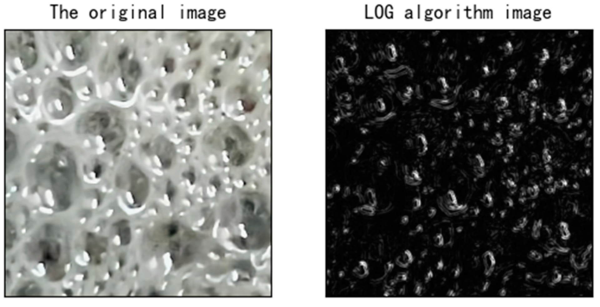
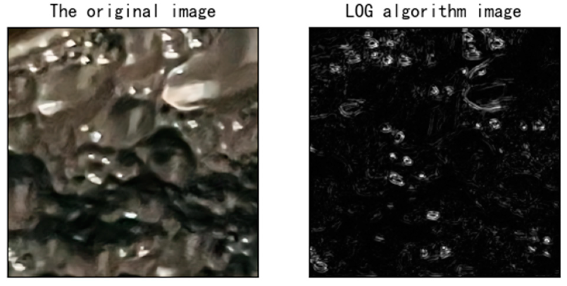
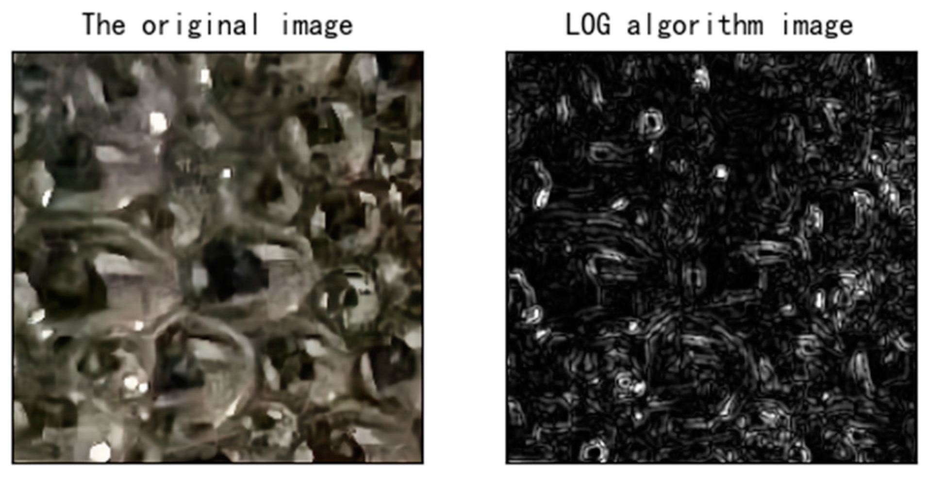
2.2.5. The LoG Edge Detection Operator

The Laplacian of Gaussian (LoG) operator is often used in edge extraction and binarization of digital images. A target image is first smoothed using a Gaussian filter, then the image Laplacian—second-order derivative—is calculated to enhance the image features. Finally, the edges are determined by detecting zero crossings—where the values of neighboring pixels change sign—in the filtered image. The zero-crossing points of the Laplacian (second-order derivative) correspond to the local maxima or minima of the first-order derivative. If necessary, the detected edge positions can be refined at the subpixel resolution level using a linear interpolation method.

The edge detection algorithm is detailed hereafter:

(1)

Image Smoothing

The image f(x, y) is smoothed with a two-dimensional Gaussian filter that approximates the characteristics of the human visual system:

$$G(x,y)=\frac{1}{2\pi \sigma }\exp (-\frac{1}{2\pi {\sigma }^2}(x^2+y^2))$$

(18)

G(x, y) is a circular symmetric function. The strength of the smoothing is controlled by the scale parameter—standard deviation—σ. A smoothed image is obtained by convolving the initial image f(x, y) with the Gaussian filter:

$$g(x,y)=f(x,y)\times G(x,y)$$

(19)

(2)

Image Enhancement

After Gaussian smoothing, the Laplacian operator is applied to the smoothed image g(x, y) to calculate the second-order image derivative:

$$h(x,y)={\nabla }^2(f(x,y)\times G(x,y))$$

(20)

(3)

Edge Detection

The edge detection criterion is a change of sign of the second-order derivative, i.e., between adjacent pixels—the zero-crossing points—in the filtered image h(x, y), corresponding to local maxima or minima of the first-order derivative. Practically, only zero-crossing points with a first-order derivative greater than a fixed threshold are selected as edge points to avoid the detection of non-significant edges. Applying the Laplacian operator to the smoothed image g(x, y) is equivalent to applying the Laplacian to the Gaussian operator and convolving the result with the initial image f(x, y). Therefore, Equation (20) is equivalent to:

$$h(x,y)=f(x,y)\times {\nabla }^{2}G(x,y)$$

(21)

${\nabla }^{2}G(x,y)$ is the LoG filter, defined as:

$${\nabla }^{2}G(x,y)=\frac{{\partial }^{2}G}{\partial x^2}+\frac{{\partial }^{2}G}{\partial y^2}=\frac{1}{\pi {\delta }^4}(\frac{x^2+y^2}{2{\delta }^2}-1)\exp (-\frac{1}{2{\delta }^2}(x^2+y^2))$$

(22)

Second-order derivative filters are very sensitive to noise. By applying a Gaussian smoothing filter before the Laplacian sharpening filter, the image noise is smoothed out before edge detection, resulting in better detection performance. Results of the edge detection algorithm for flotation foam images of scheelite, coal gangue and lead-zinc ore are shown in Figure 6, Figure 7 and Figure 8, respectively.

2.3. Screening and Analysis of Factors Influencing the Flotation Process

2.3.1. Image Preprocessing

(1)

Grayscale Transformation

A grayscale transformation is a point-by-point image transformation that corrects the pixel gray values of the original input image to determine a corresponding output gray value for each pixel. The general expression is:

$$s=T(r)$$

(23)

where T is the grayscale transformation function, R is the matrix of gray level values before transformation, and S is the output matrix containing the transformed gray values.

If T is determined, then the output gray values are also known. The properties of function T determine the effect of the grayscale transformation.

(2)

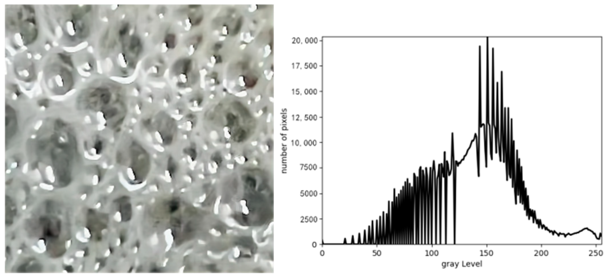
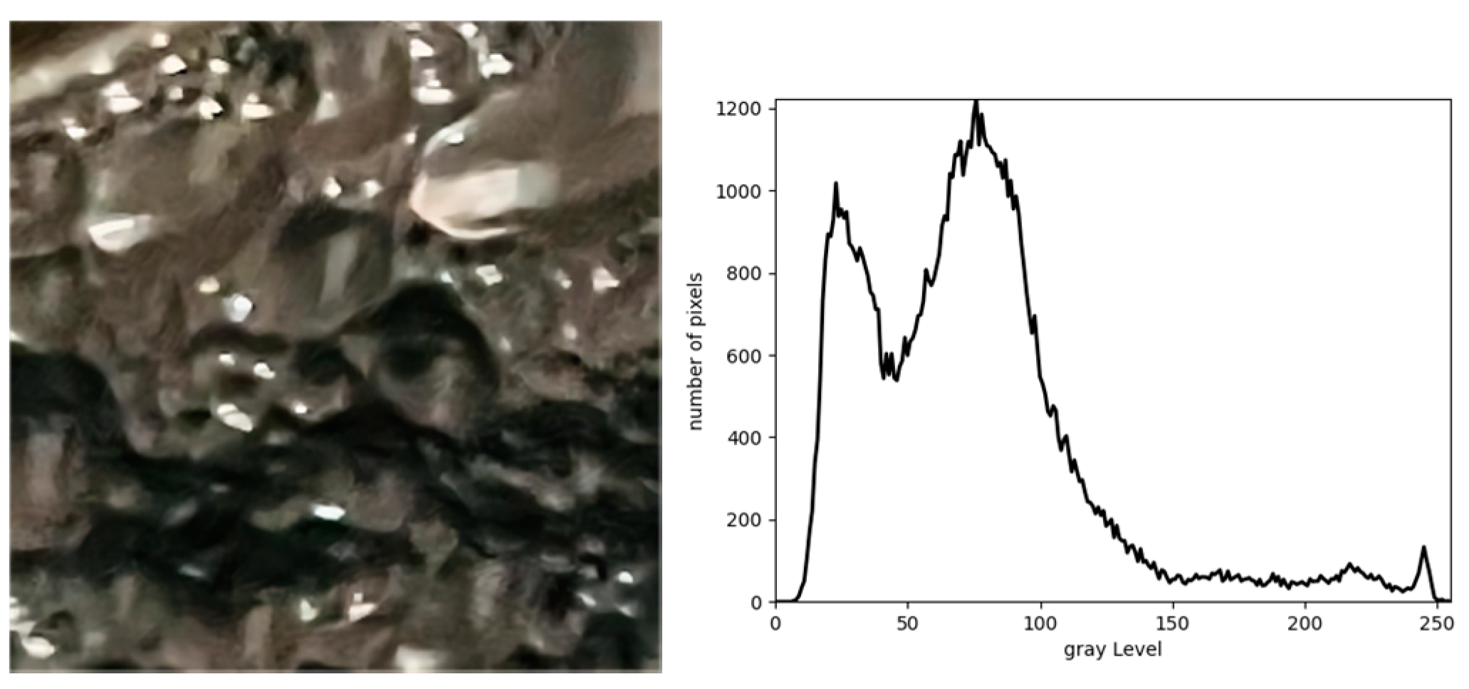
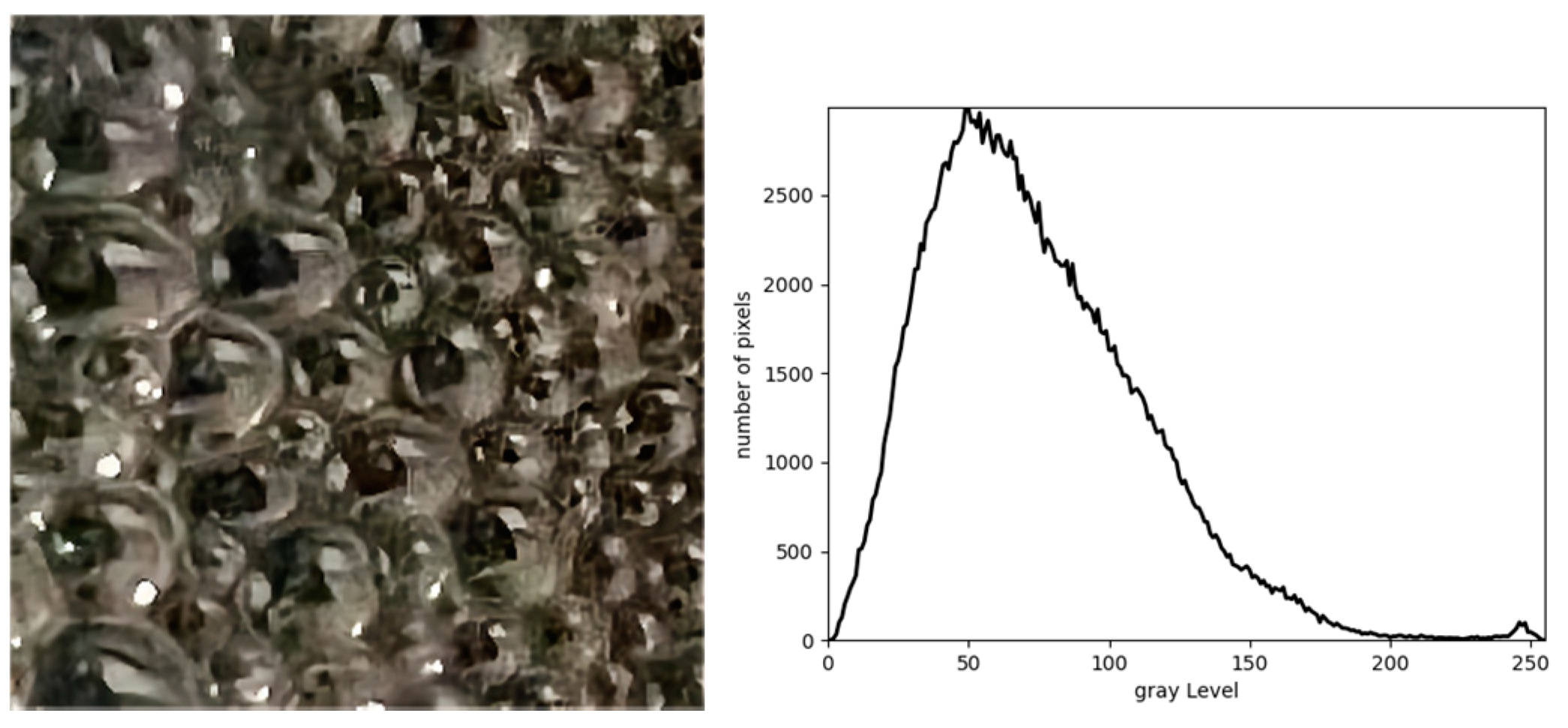
Gray-Level Histogram

The histogram of a grayscale image counts the number of image pixels for each gray level value. When divided by the total number n of image pixels, the resulting normalized histogram also represents the probability density function p(r_k)—in the interval [0, 1]—for each gray value r_k and directly reflects the occurrence probability of each gray value. For an image with n = 256, if n_k is the number of pixels with a gray value r_k, then the occurrence probability of r_k is:

$$p(r_k)=\frac{n_k}{n},(k=0,1,\cdots ,L-1,n_k\ge 0)$$

(24)

where L represents the odd gray level in the image.

The histogram is easily calculated by counting the number of pixels for each gray level and sorting them in ascending order of gray value. The Open Source Computer Vision (OpenCV) library is a software package dedicated to machine vision and developed for the Python open-source programming language. OpenCV provides a histogram calculation function (calcHist) that calculates gray-level histograms for multiple images, multiple channels and different ranges of gray values simultaneously. The histograms calculated with calcHist for flotation foam images of scheelite, coal gangue and lead-zinc ore are shown in Figure 9, Figure 10 and Figure 11, respectively.

Histograms form the basis of image recognition. Figure 9, Figure 10 and Figure 11 clearly show marked histogram differences between the gray-level distributions of the three flotation foams. Such information is fundamental for parameter adjustment in the next image processing step, thereby strongly improving the efficiency and accuracy of the image recognition algorithm.

2.3.2. Linear Regression Model for Factors Influencing the Flotation Process

NumPy is the most widely used numerical analysis library for scientific computing in Python. NumPy provides high-level mathematical functions and algorithms and is very useful to build linear regression models. Furthermore, to eliminate model errors caused by algorithm randomness, the scikit-learn package—a Python package for machine learning—was used to simulate observations, train and evaluate the model independently, and assess the possibilities for further model optimization [26,27]. Unary linear regression models for light and noise intensity were built and trained on the dataset. Output models derived for light and noise intensity from 1000 simulation experiments are shown in Figure 12 and Figure 13, respectively.

There are discrepancies between the regression models and the data, notably for the noise intensity. This is expected because light and noise intensity are only two of the main factors affecting image segmentation. Without accounting for other factors such as dosage, pulp density, wind pressure, and foam layer thickness, the fitted values necessarily differ from the original data. To evaluate the quality of the regression models and the correlation between influencing factors and segmentation accuracy, the goodness-of-fit is estimated from the coefficient of determination and the linear correlation is evaluated from the correlation coefficient. Results for the light and noise intensity models are shown in

Table 2. Coefficients of determination and correlation coefficients for both regression models.

Influence Factor	Coefficient of Determination	Coefficient of Association
Noise intensity	0.6764	−0.7639
Light intensity	0.9431	−0.9169

.

Table 2 shows that the coefficient of determination for light intensity is higher than 0.9, indicating high goodness-of-fit, whereas the coefficient of determination for noise intensity is lower than 0.7, indicating low goodness-of-fit. The absolute value of the correlation coefficient for light intensity is also higher than 0.9, indicating a strong linear correlation. The corresponding value for noise intensity is higher than 0.75, also showing a good linear correlation. However, because of the low goodness-of-fit for the noise intensity regression model (67.64%), only light intensity is considered hereafter.

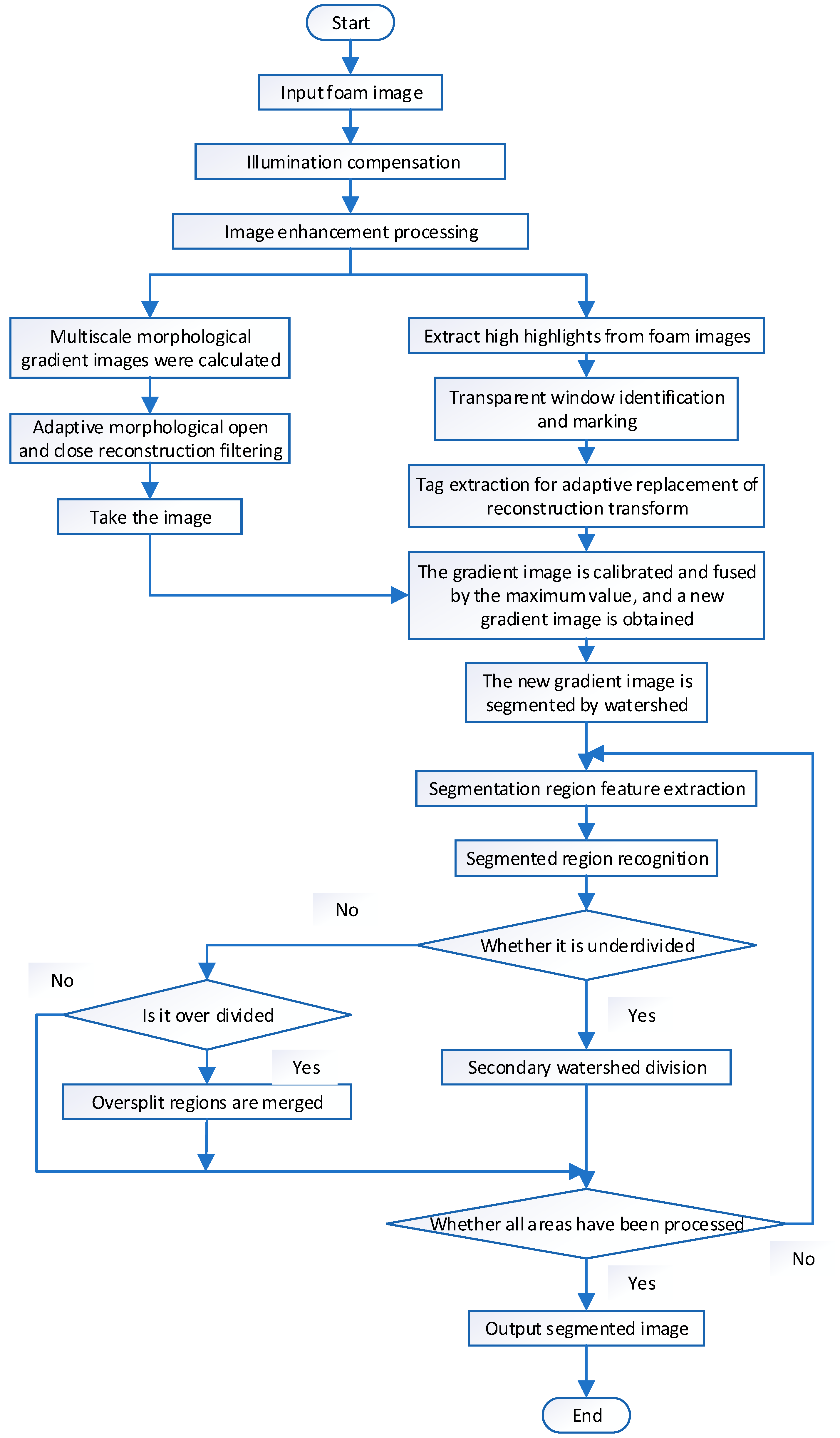
3. Improvement of the Watershed Segmentation Algorithm Using the OpenCV Library

Image segmentation is an important part of image analysis. To retrieve and measure all features of interest from the full image, the original must be separated into meaningful subsets or regions.

3.1. The OpenCV Watershed Segmentation Algorithm

The purpose of image thresholding is to separate the pixel set into subsets defined by their gray level value, with each subset or region corresponding to the real scene. Each region is described by consistent internal attributes that are different from those of adjacent regions. Subsetting can be achieved by selecting appropriate gray-level thresholds [28].

The watershed algorithm in OpenCV improves on the original algorithm by adding a preprocessing step: converging and non-converging valleys are selected before segmentation. To avoid a known oversegmentation issue affecting the original watershed algorithm, OpenCV uses a series of predefined markers to guide the image segmentation definition. As input, the OpenCV algorithm requires a labeled image for which pixel gray values are 32-bit signed positive numbers and each non-zero pixel represents a label.

During the segmentation process, the top regions of the bubbles are identified first and optimal structural elements are selected using an adaptive segmentation parameter selection method. Then, the output of the watershed algorithm is obtained by morphological processing of the foam image, which becomes coarsely segmented.

Uneven bubble mixing produces under- and oversegmented regions. To minimize this effect, we use a fuzzy texture spectrum algorithm—with good real-time texture feature extraction and area segmentation (fuzzy c-means clustering algorithm)—and a support vector machine for regional identification. After identifying undersegmented and oversegmented areas, finer segmentation is applied to the undersegmented areas. This method can effectively be used to solve the problem of inappropriate segmentation [29].

3.2. Flow Improvement for the OpenCV Watershed Segmentation Algorithm

As mentioned in Section 3.1, the foam image is first clustered with the Fuzzy C-means clustering algorithm—implemented in the “fuzzy-c-means” Python module [30]—and the top regions of the bubbles are identified. An adaptive segmentation parameter selection method is used to select the optimal structural elements, morphological processing is applied to the foam image to derive the watershed algorithm output image, then the foam image becomes coarsely segmented. The algorithm flow is shown in Figure 14.

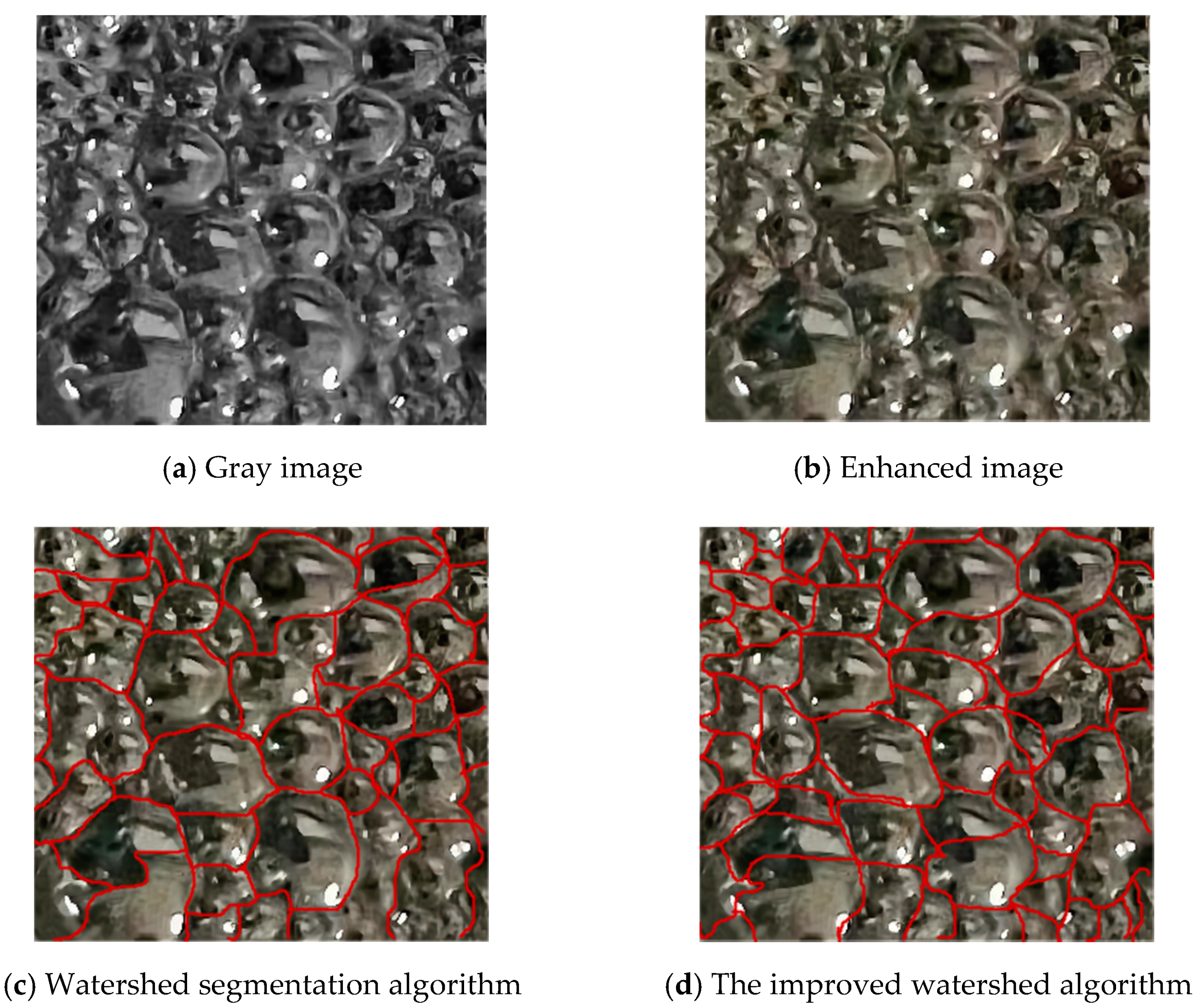
3.3. Comparison of Experimental Results from Segmentation Simulations

For this analysis, a library of 80 flotation foam images acquired in December 2021 was selected from the image database of a lead-zinc mine in Yunnan Province. The selected images were extracted from video footage recorded during two work shifts in different working conditions. Because the images show a flotation foam without background non-uniform adhesion, segmentation must meet the real-time performance requirements of the flotation process. To evaluate the segmentation performance, this manuscript compares the original and improved versions of the OpenCV watershed segmentation algorithm with the result of expert manual segmentation.

Full evaluation of the algorithm performance includes a subjective evaluation and an objective assessment. The subjective evaluation is conducted by skilled personnel who visually evaluate the segmentation results. The objective evaluation is a statistical analysis of the automatic segmentation results using expert manual segmentation as a reference. A segmentation evaluation index k is defined to compare the automatic segmentation algorithms and the manual segmentation reference:

$$k=2\times \frac{N\left(M{{\displaystyle \cap }}^{\text{}}S\right)}{N\left(M\right)+N\left(S\right)}\times 100\%$$

(25)

Here, M and S are the results from expert manual segmentation and from the automatic segmentation algorithms, respectively; the intersection M∩S represents the segmentation regions common to the manual and automatic results; and N represents the number of regions identified during the manual—N(M)—and automatic—N(S)—segmentation experiments or common to both—N(M∩S). Operation time is also compared.

An image acquired in typical working conditions is randomly selected from the 80-image library for a segmentation simulation. The original gray image is shown in Figure 15a and the enhanced image after Retinex compensation is shown in Figure 15b. Segmentation results for the standard watershed segmentation algorithm are shown in Figure 15c. Results for the improved watershed segmentation algorithm proposed in this paper, after enhancement with the Retinex image compensation method, are shown in Figure 15d. For the selected image, representative of typical working conditions, the standard watershed algorithm segments the foam image into 55 bubbles, but the improved watershed algorithm yields 66 bubbles.

The difference between the standard and improved versions of the watershed segmentation algorithm is apparent in Figure 15c,d. Both versions yield good results, with generally accurate segmentation of the foam image into conventional regions. In good working conditions, segmentation results are similar for both algorithms. However, the selected image (Figure 15a) includes several bright spot areas near the edges of the frame. In this case, operating assumptions for the watershed algorithm are not met. Thus, uneven illumination causes improper segmentation for both algorithm versions relative to the manual segmentation reference, but with comparatively better performance of the improved watershed algorithm. The improved algorithm developed in this work is markedly more robust and accurate, and yields results closer to manual segmentation. Therefore, it is more suitable for foam image segmentation under less favorable working conditions.

3.4. Statistical Analysis of the Segmentation Simulation Results

Simulation results for the standard and improved versions of the watershed segmentation algorithm are given in

Table 3. Evaluation of the segmentation results for the standard watershed algorithm and for the improved version defined in this work.

Algorithm	Mean Split Time (s)	Average Segmentation Accuracy (%)
Watershed algorithm	5.863	88.73
Improved watershed algorithm	5.285	92.06

.

To compare the real-time performance of both algorithms, 50 flotation foam images were randomly selected for segmentation from the image library. To reduce the manual segmentation error, the results of five manual segmentation operations were averaged to produce a reference segmented image. Segmentation accuracy relative to the reference and operation time is calculated for both algorithms. As seen in Table 3, the accuracy of the improved watershed algorithm is 3.3% higher than that of the standard algorithm and the operation time is reduced by 9.9%. Segmentation results from both algorithms are comparable when the image is segmented. However, the proposed algorithm is faster and yields markedly higher segmentation accuracy for non-uniform flotation foam images under fluctuating working conditions.

4. Conclusions

During the industrial mineral flotation process, bubble size and morphology reflect real-time changes in the flotation conditions. Accurate foam image segmentation algorithms must be able to adapt to such fluctuating conditions. In this paper, we proposed an improved version of the watershed segmentation algorithm implemented in the OpenCV library of the versatile, open-source Python programming language. The improved algorithm was applied to flotation foam images and segmentation results were compared with results from the OpenCV standard watershed segmentation algorithm and from manual segmentation.

(1)

First, the flotation foam images were enhanced with the Retinex image compensation method—also implemented in a Python module. Strong-contrast area recognition and illumination compensation of the flotation foam image were improved, with a better visual result and more possibilities to extract useful details from the foam image.

(2)

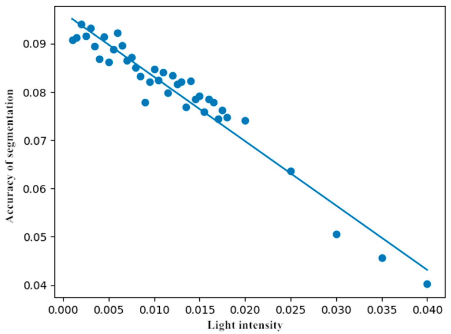
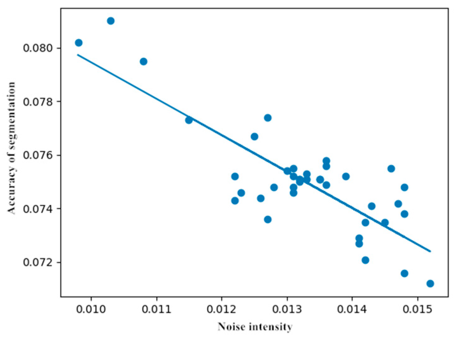
A linear regression model was developed, also in Python, to analyze major factors influencing the segmentation accuracy. Application of the model to light and noise intensity showed that both factors had an influence on flotation foam segmentation, larger for light intensity.

(3)

The improved version of the OpenCV watershed segmentation algorithm proposed in this paper, also written in Python, yielded better results than the standard version. Segmentation time was 3.3% shorter and segmentation accuracy increased by 9.9%. Comparison with results from the standard watershed algorithm and from manual segmentation showed that the proposed algorithm is accurate and robust.

References

1. Beneventi, D.; Benesse, M.; Carré, B.; Saint Amand, F.J.; Salgueiro, L. Modelling Deinking Selectivity in Multistage Flotation Systems. Sep. Purif. Technol. 2007, 54, 77–87. [Google Scholar] [CrossRef]
2. Bergh, L.; Yianatos, J. The Long Way Toward Multivariate Predictive Control of Flotation Processes. J. Process Control 2011, 21, 226–234. [Google Scholar] [CrossRef]
3. Aldrich, C.; Marais, C.; Shean, B.; Cilliers, J. Online Monitoring and Control of Froth Flotation Systems with Machine Vision: A Review. Int. J. Miner. Process. 2010, 96, 1–13. [Google Scholar] [CrossRef]
4. Moolman, D.W.; Eksteen, J.J.; Aldrich, C.; Van Deventer, J.S.J. The Significance of Flotation Froth Appearance for Machine Vision control. Int. J. Miner. Process. 1996, 48, 135–158. [Google Scholar] [CrossRef]
5. Bonifazi, G.; Serranti, S.; Volpe, F.; Zuco, R. Characterisation of flotation froth colour and structure by machine vision. Comput. Geosci. 2001, 27, 1111–1117. [Google Scholar] [CrossRef]
6. Shean, B.; Cilliers, J. A Review of Froth Flotation Control. Int. J. Miner. Process. 2011, 100, 57–71. [Google Scholar] [CrossRef]
7. Kaartinen, J.; Hätönen, J.; Hyötyniemi, H.; Miettunen, J. Machine-Vision-Based Control of Zinc Flotation—A Case Study. Control Eng. Pract. 2006, 14, 1455–1466. [Google Scholar] [CrossRef]
8. Van Brown, O.; Bourke, R.J.A. Improving Flotation Plant Performance at Cadia by Controlling and Optimising the Rate of Froth Recovery Using Outokumpu Frothmaster. Australas. Inst. Min. 2000, 6, 127–135. [Google Scholar]
9. Bonifazi, G.; Giancontieri, V.; Meloni, A.; Serranti, S.; Volpe, F.; Zuco, R.; Koivo, H.; Hätönen, J.; Hyötyniemi, H.; Niemi, A.; et al. Characterization of the Flotation Froth Structure and Color by Machine Vision (ChaCo). Dev. Miner. Process. 2000, 13, C8a–39. [Google Scholar]
10. Wang, W.X.; Stephansson, O.; Wan, S.C. On-Line System Setup in a Cellar of a Flotation Plant. In Proceedings of the 15th International Conference on Pattern Recognition. ICPR-2000, Barcelona, Spain, 3–7 September 2000; Volume 4, pp. 791–794. [Google Scholar]
11. Wang, W.; Stephansson, O.A. Robust Bubble Delineation Algorithm for Froth Images. In Proceedings of the Second International Conference on Intelligent Processing and Manufacturing of Materials. IPMM’99 (Cat. No.99EX296), Honolulu, HI, USA, 10–15 July 1999; Volume 1, pp. 471–476. [Google Scholar]
12. Citir, C.; Aktas, Z.; Berber, R. Off-Line Image Analysis for Froth Flotation of Coal. Comput. Chem. Eng. 2004, 28, 625–632. [Google Scholar] [CrossRef]
13. Sadr-Kazemi, N.; Cilliers, J. An Image Processing Algorithm for Measurement of Flotation Froth Bubble Size and Shape Distributions. Miner. Eng. 1997, 10, 1075–1083. [Google Scholar] [CrossRef]
14. Forbes, G.; De Jager, G. Texture Measures for Improved Watershed Segmentation of Froth Images. In Fifteenth Annual Symposium of the Pattern Recognition Association of South Africa; OpenUCT: Cape Town, South Africa, 2004; pp. 1–6. [Google Scholar]
15. Zhang, H.; Tang, Z.; Xie, Y.; Gao, X.; Chen, Q. A Watershed Segmentation Algorithm Based on an Optimal Marker for Bubble Size Measurement. Measurement 2019, 138, 182–193. [Google Scholar] [CrossRef]
16. Lézoray, O.; Charrier, C. Color Image Segmentation Using Morphological Clustering and Fusion with Automatic Scale Selection. Pattern Recognit. Lett. 2009, 30, 397–406. [Google Scholar] [CrossRef]
17. Marais, C.; Aldrich, C. Estimation of Platinum Flotation Grades from Froth Image Data. Miner. Eng. 2011, 24, 433–441. [Google Scholar] [CrossRef]
18. Henry, T.; Ngan, Y.; Grantham, H.; Pang, K.; Nelson, C. Computing, Automated fabric defect detection—A Review. Image Vis. Comput. 2011, 29, 442–458. [Google Scholar]
19. Bask, M.; Johansson, A. Robust Time-Varying Thresholds for Supervision of Valves in a Flotation Process. In Proceedings of the 2004 43rd IEEE Conference on Decision and Control, Nassau, Bahamas, 14–17 December 2004. [Google Scholar]
20. Liu, J.J.; MacGregor, J.F. Froth-Based Modeling and Control of Flotation Processes. Miner. Eng. 2008, 21, 642–651. [Google Scholar] [CrossRef]
21. Kim, J.; Fisher, J.; Yezzi, A.; Cetin, M.; Willsky, A. A Nonparametric Statistical Method for Image Segmentation Using Information Theory and Curve Evolution. IEEE Trans. Image Process. 2005, 14, 1486–1502. [Google Scholar] [CrossRef]
22. Torralba, A.; Oliva, A. Statistics of Natural Image Categories. Netw. Comput. Neural Syst. 2003, 14, 391. [Google Scholar] [CrossRef]
23. Land, E.H. An Alternative Technique for the Computation of the Designator in the Retinex Theory of Color Vision. Proc. Natl. Acad. Sci. USA 1986, 83, 3078–3080. [Google Scholar] [CrossRef]
24. Kimmel, R.; Elad, M.; Shaked, D.; Keshet, R.; Sobel, I. A Variational Framework for Retinex. Int. J. Comput. Vis. 2003, 52, 7–23. [Google Scholar] [CrossRef]
25. Hao, W.; He, M.; Ge, H.; Wang, C.-J.; Gao, Q.-W. Retinex-Like Method for Image Enhancement in Poor Visibility Conditions. Procedia Eng. 2011, 15, 2798–2803. [Google Scholar] [CrossRef]
26. Swami, A.; Jain, R.J. Scikit-Learn: Machine Learning in Python. J. Mach. Learn. Res. 2013, 12, 2825–2830. [Google Scholar]
27. Güney, Y.; Bozdogan, H.; Arslan, O. Robust Model Selection in Linear Regression Models Using Information Complexity. J. Comput. Appl. Math. 2021, 398, 113679. [Google Scholar] [CrossRef]
28. A Full Color Digital Imaging Based Approach to Characterize Flotation Froth: An Experience in Pyhasalmi (SF) and Garpenberg (S)Plants. In In Proceedings of the Beijing International Conference on Imaging Technology and Applications in the 21st Century, Beijing, China, 23–26 May 2005.
29. Luo, J.; Tang, Z.; Zhang, H.; Fan, Y.; Xie, Y. LTGH: A Dynamic Texture Feature for Working Condition Recognition in the Froth Flotation. IEEE Trans. Instrum. Meas. 2021, 70, 1–10. [Google Scholar] [CrossRef]
30. Kuo, B.-C.; Huang, W.-C.; Liu, H.-C.; Tseng, S.-C. A Novel Fuzzy C-Means Method for Hyperspectral Image Classification. IEEE Int. Geosci. Remote Sens. Symp. 2008, 2, II-1002–II-1005. [Google Scholar] [CrossRef]
Figure 1. Schematic diagram of statistical image modeling by parameter quantization.
Minerals 12 01126 g001
Figure 2. Gray levels and pixel value information for a foam image.
Minerals 12 01126 g002
Figure 3. Sampled image of a scheelite flotation foam (left) and the corresponding Fourier-transform spectrum ((right), with x, y and z in arbitrary units).
Minerals 12 01126 g003
Figure 4. Sampled image of a coal gangue flotation foam (left) and the corresponding Fourier-transform spectrum ((right), with x, y and z in arbitrary units).
Minerals 12 01126 g004
Figure 5. Sampled image of a lead-zinc ore flotation foam (left) and the corresponding Fourier-transform spectrum ((right), with x, y and z in arbitrary units).
Minerals 12 01126 g005
Figure 6. Original image of a scheelite flotation foam (left) and result of the LoG detection algorithm (right).
Minerals 12 01126 g006
Figure 7. Original image of a coal gangue flotation foam (left) and result of the LoG detection algorithm (right).
Minerals 12 01126 g007
Figure 8. Original image of a lead–zinc ore flotation foam (left) and result of the LoG detection algorithm (right).
Minerals 12 01126 g008
Figure 9. Original image of a scheelite flotation foam (left) and the corresponding histogram (right).
Minerals 12 01126 g009
Figure 10. Original image of a coal gangue flotation foam (left) and the corresponding histogram (right).
Minerals 12 01126 g010
Figure 11. Original image of a lead-zinc ore flotation foam (left) and the corresponding histogram (right).
Minerals 12 01126 g011
Figure 12. Influence of light intensity on segmentation accuracy and the linear regression model.
Minerals 12 01126 g012
Figure 13. Influence of noise intensity on segmentation accuracy and the linear regression model.
Minerals 12 01126 g013
Figure 14. Flowchart of the improved OpenCV watershed segmentation algorithm.
Minerals 12 01126 g014
Figure 15. Flotation foam image segmentation simulation. (a) Gray image; (b) Enhanced image; (c) Watershed segmentation algorithm; (d) The improved watershed algorithm.
Minerals 12 01126 g015