Hybrid Serving of DOE and RNN-Based Methods to Optimize and Simulate a Copper Flotation Circuit

Abstract

Prediction of metallurgical responses during the flotation process is extremely vital to increase the process efficiency using a proper modeling approach. In this study, two new variants of the recurrent neural network (RNN) method were used to predict the copper ore flotation indices, i.e., grade and recovery within different operating conditions. The model input parameters including pulp pH and solid content as well as frother and collector dosages were first analysed and then optimized using a two-step factorial approach. The statistical analysis showed a reliable correlation between operating parameters and copper grade and recovery with coefficients of 99.86% and 94.50%, respectively. The main effect plots indicated that pulp pH and solid content positively affect copper grade while increasing the frother and collector dosages negatively influenced the quality of the final concentrate. Despite the same effect from pulp pH, reverse effects from other variables were observed for copper recovery. Process optimization revealed that maximum copper recovery of 44.39% with a grade of 11.48% could be achieved under the optimal condition as pulp pH of 10, solid content of 20%, and frother and collector concentrations of 25 g/t and 9.9 g/t, respectively. Then, the predictive efficiency of long short-term memory (LSTM) and gated recurrent unit (GRU) networks with proper structure were evaluated using mean square error (MSE), root mean square error (RMSE), mean absolute percentage error (MAPE), and correlation coefficient (R²). The simulation results showed that the LSTM network with higher R² of 0.963 and 0.934 for copper grade and recovery, respectively, was more effective than the GRU algorithm with the corresponding values of 0.956 and 0.919, respectively. The results show that the LSTM model could be useful in predicting the copper flotation behaviour in response to changes in the operating parameters.

1. Introduction

Nowadays, simulation and modelling science are widely used as a reliable, fast, and low-cost solution to predict the behaviour of mineral processing units. Using simulations and modelling before or instead of experimental studies involving a large number of laboratory tests can significantly reduce executive and manpower costs. Furthermore, the flexibility of such approaches makes it possible to change or modify various stages of the process design without the need for a significant change in the initial redesign [1,2]. So far, several methods have been developed for modelling and simulation of mineral processing units, of which empirical and semi-empirical types and statistical models are the most common.

Despite the widespread use of these models, especially in simulation software development, each of the above approaches is associated with limitations that make their application in real operational environments challenging. For example, empirical and semi-empirical parametric models are developed based on a series of data sets from a specific process or multiple processes. Therefore, their use in new processes with different operating conditions leads to inefficiency and reduced accuracy in some cases. However, most models have tried to manage this limitation to some extent by considering the calibration coefficients [3,4]. The development of statistical models is easier than empirical models. However, the most important challenge of statistical models, in addition to being limited to the initial data of model development, is to include parameters that usually lack physical meaning. For example, variables that are the product of more than two major effects (the primary variable) and are abundantly observed in the design of experiment (DOE)-based models and cannot be interpreted in the model [5,6]. Besides, although mineral processing processes have relatively simple mechanical and physical aspects, they have very complex mechanisms, some of which still remain unknown. Metallurgical and operational factors as well as their interactions are major factors responsible for such complexities. As such, modelling and simulation of these processes have always posed a controversial topic.

In recent years, the use of expert system methods (ESM) such as artificial neural networks, and genetic algorithms have been proposed to simulate complicated separation techniques [7,8,9]. Intelligent algorithms process experimental data and transmit underlying knowledge in order to create a network structure. It is possible to apply ESM to implement intricate functions in a wide range of fields such as process automation, control and monitoring, medical diagnosis, and image analysis. Nowadays, we can solve difficult problems for humans and usual computers using efficiently trained intelligent algorithms [10,11,12]. Forecasting with ESMs has been one of the main uses of the algorithms, which have also shown excellent results. The good performance of ESMs has made them popular in different scientific fields, including mining and mineral processing. For instance, Jorjani et al. [13] used artificial neural networks to simulate the process of leaching rare earth elements from apatite concentrate on an industrial scale and showed that a reasonably accurate model could be developed using the improved ANN algorithm. In a later study, Milivojevic et al. [14] simulated the nickel ore leaching process to demonstrate that expert systems are more reliable than linear regression-based statistical models. In another research, Hoseinian et al. [15] used a hybrid neural-genetic algorithm to simulate copper recovery during a column leaching process of a copper ore sample on a pilot scale, and found that using an appropriate algorithm could yield reliable prediction results. In a recent study, using hybrid artificial neural networks and particle swarm optimization (PSO), Sobouti et al. [16] simulated lead recovery during the leaching of lead concentrate. The noteworthy aspect of the study was the wide range of operating parameters used in the simulation, such as temperature, liquid/solid ratio, stirring speed, fluoroboric acid concentration, and leaching time. They showed that an effective simulation of the process could be achieved using an optimized ANN-PSO algorithm. Artificial neural networks have also been successfully used to simulate mineral processing operations reported by Vyas et al. [17]. In their study, ANN was used to simulate and predict the spent catalyst bioleaching process with acceptable accuracy, and simulation results were presented in both numerical and graphical forms. According to Ghobadi et al. [18], the copper flotation circuit was modelled and optimized simultaneously using a genetic algorithm. They found that in comparison to conventional mathematical methods, an oriented genetic algorithm reduces the calculation time by 1/60 for a two-stage flotation system and can provide higher optimization accuracy. In another study, Gholami and Khoshdast [19] found that with a limited number of operating data, multiple metallurgical responses of the bioflotation process of coal can be accurately simulated using the ANN method. Their investigation into different algorithms for developing the ANN model demonstrated that the simulation accuracy is greatly influenced by the choice of the network algorithm. Recently, Gholami et al. [20] coupled historical data and deep learning techniques to predict the flotation behaviour of a copper mine in response to mineralogical and operational variables. They showed that mixed statistical/intelligent methods can be a promising approach to accurately simulate the flotation process with an accuracy of more than 95%.

The effective application of the recurrent neural network (RNN) method has also been reported by a few researchers. For example, radial basis function neural network, recurrent neural network, and multivariate nonlinear regression have been used to predict the metallurgical performance of the flotation column [21]. It was shown that the recurrent neural network forecasted the metallurgical performance of the flotation column better than the radial basis function neural network and multivariate nonlinear regression models. The same conclusions have also been recently reported by some other researchers [22,23] to estimate the mineral grade in the field of flotation. Inapakurthi et al. [24] proposed a method using RNN for simulation of industrial grinding circuit in the lead–zinc ore beneficiation process. They also demonstrated that the RNN model can successfully control a GC while tracking its set point without violating any constraints.

The main conclusion stemming from the above studies is that intelligent modelling methods along with limited amount of data of operational/process parameters can be used to simulate mineral processing operations successfully. Considering the results reported in the above studies, the simulation has a high degree of accuracy in most cases, which is highly desirable from an application perspective [25]. Hence, in this study, a mid-size copper mineral processing plant was targeted to intelligent simulation using long short-term memory (LSTM) and gated recurrent unit (GRU) networks as two well-known RNN methods. Among intelligent modelling methods for time series and sequential data predictions, RNNs are the commonly used ones. LSTM and GRU have a similar overall structure, but LSTM is more complex. Therefore, in addition to accurate prediction of output variables, a comparison of these two methods is also considered in this paper. The main parameters on the efficiency of the flotation process including pulp pH, solid content, and concentrations of frother and collector were first optimized by the DOE method and then, were considered as inputs in the model. Moreover, an accuracy analysis was performed to investigate the reliability of copper grade and recovery prediction.

2. Materials and Methods

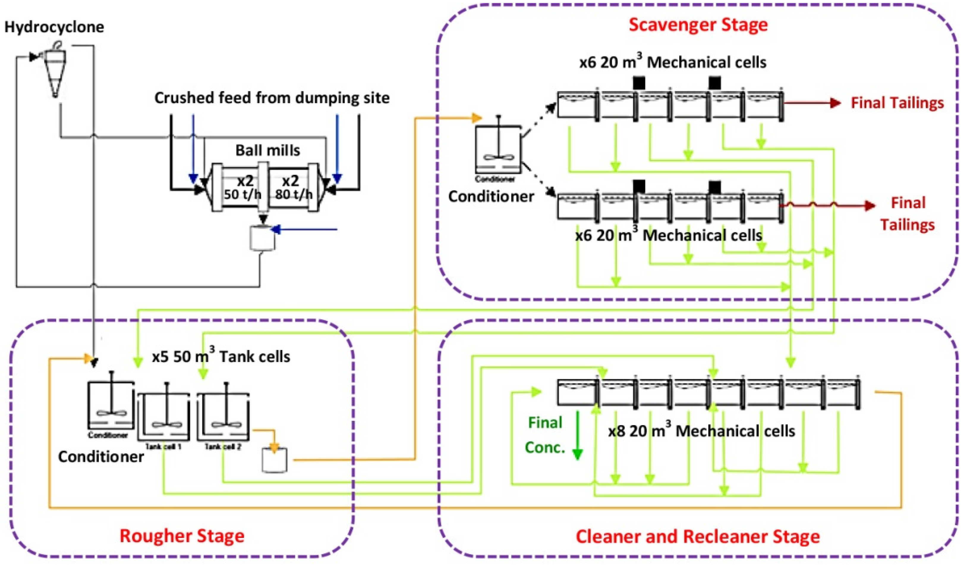
2.1. A Brief Description of the Processing Plant

Studies were performed in the Takht Gonbad copper processing plant (Sirjan, Iran). With a practical capacity of 230 t/h, this plant beneficiates a copper sulfidic ore with an average copper grade of 0.45% to a concentrate with a grade of 22 ± 2% through several stages of roughing and cleaning. The copper grade in the final tailings of this plant is about 0.1%. According to Figure 1, the crushed ore is first broken down by four ball mills with capacities of 50 to 80 t/h to reduce the particle sizes to 80% finer than 100 μm. Comminuted particles are fed to the hydrocyclone unit, classifying them into two fine and coarse parts. The hydrocyclone overflow, consisting of particles 80% finer than 75 μm, is directed to a conditioning tank with a capacity of 50 m³ to prepare the feed for the flotation circuit. At this stage, flotation reagents including sodium isopropyl xanthate (Z11) and sodium dithiophosphate (DTU) as copper mineral collectors, methyl isobutyl carbinol (MIBC) and a polypropylene glycol with molecular weight of 395.61 g/mol (A65) as frothers, lime as pH regulator, and NaHS as pyrite depressant (according to the mineralogical composition of the input feed) are added to the pulp. The concentration of reagents is adjusted according to the metallurgical conditions of the plant. The range of changes in the amount of consumption of these reagents is presented in

Table 1. Operating factors and their levels studied in the screening experimental design.

Factor	Variable	Unit	Low Actual	High Actual	Mid Level	Std. Dev.
A	pH	-	10	12	11	0.85
B	Solid content	(%)	20	30	25	4.26
C	MIBC conc.	(g/t)	5	35	20	12.79
D	A65 conc.	(g/t)	5	15	10	4.26
E	DTU conc.	(g/t)	5	35	20	12.79
F	Z11 conc.	(g/t)	5	25	15	8.53
G	NaHS conc.	(g/t)	0	10	5	4.26

. Prepared pulp with a solid content of about 25% (w/w) is first introduced into the rougher line with five 50 m³ tank cells. The concentrate of this step is directed to an eight-cell row, including four cleaner and four recleaner cells to increase the copper grade. The final concentrate of this stage leaves the circuit as the final concentrate after several stages of recirculation in the cleaning circuit. The tailing is also returned to the beginning of the rougher circuit. Rougher tailing transfers to the scavenging circuit consisting of two 6-cell rows. The tailing of this unit is considered the final tailings of the plant, but the concentrate of the first two cells from both lines is returned to the cleaning circuit, and the concentrate of the last four cells is fed to the rougher circuit.

2.2. Ore Sample and Reagents Used

A representative sample was taken from the hydrocyclone overflow as the feed of the flotation circuit (Figure 1) to determine the physical and mineralogical characteristics of the studied ore. Samples were collected using an automatic scoop sampler with an adjustable container size. Light microscopy (Axio Imager 2 Pol, Zeiss, Jena, Germany) was used to determine the mineralogical composition of the ore. The particle size distribution of the sample was measured using the standard dry sieve analysis method. All the applied reagents, including MIBC and A65 frothers, Z11 and DTU collectors, and NaHS depressant were sourced from the company’s warehouse.

2.3. Screening of Operational Variables

Due to the variety of the operating parameters, first, the effectiveness of each operational variable was evaluated using a fractional factorial experimental design utilizing Design-Expert software (Demo version 7.0.0, from Stat-Ease Inc., Minneapolis, MN, USA). The levels of each variable were selected based on monitoring the process over six months (autumn and winter 2021). Table 1 lists the variables and their levels considered in the screening design. The experimental design used for screening studies and their practical results are presented in

Table 2. The structure and practical results of the screening experimental design.

	Operating Factors							Responses
Run	A: pH	B: Solid Content (%)	C: MIBC (g/t)	D: A65 (g/t)	E: DTU (g/t)	F: Z11 (g/t)	G: NaHS (g/t)	Cu Grade (%)	Cu Recovery (%)
1	10	20	35	15	5	5	10	4.90	71.53
2	12	20	35	5	35	5	0	4.90	86.87
3	11	25	20	10	20	15	5	3.60	53.88
4	10	30	5	5	35	5	10	2.96	64.92
5	12	30	35	15	35	25	10	4.30	44.00
6	10	20	5	15	35	25	0	4.70	58.28
7	12	30	5	15	5	5	0	4.40	58.17
8	12	20	5	5	5	25	10	5.20	55.82
9	11	25	20	10	20	15	5	2.60	62.42
10	12	30	5	15	5	5	0	4.80	59.59
11	12	20	35	5	35	5	0	5.10	68.90
12	10	20	35	15	5	5	10	5.17	56.97
13	12	30	35	15	35	25	10	4.60	50.91
14	10	30	35	5	5	25	0	3.57	52.75
15	11	25	20	10	20	15	5	3.15	58.14
16	11	25	20	10	20	15	5	3.10	58.83
17	12	20	5	5	5	25	10	4.90	58.38
18	10	20	5	15	35	25	0	4.50	68.48
19	11	25	20	10	20	15	5	2.44	41.96
20	10	30	35	5	5	25	0	3.61	53.32
21	11	25	20	10	20	15	5	3.54	62.53
22	10	30	5	5	35	5	10	2.78	59.05

. These studies evaluated the grade and recovery of copper in the rougher stage concentrate as the process responses.

2.4. Statistical Optimization Studies

Influential operating variables for optimization studies were selected according to the results of the screening studies as listed in

Table 3. Operating factors and their levels studied in the optimization experimental design.

Factor	Parameter	Unit	Low Level	High Level	Mid Level	Std. Dev.
A	pH		10	12	11	0.92
B	Solid Content	(%)	10	20	15	4.59
C	A65 Conc.	(g/t)	10	25	17.5	6.88
D	Z11 Conc.	(g/t)	0	20	10	9.18

. Then, a full factorial design was used to investigate the real impact of each parameter, their interactions, as well as process optimization. The optimization design with practical results is presented in

Table 4. The structure and practical results of the optimization experimental design.

	Operating Factors				Responses
Run	A: pH	B: Solid Content (%)	C: A65 (g/t)	D: Z11 (g/t)	Cu Grade (%)	Cu Recovery (%)
1	11	15	17.5	10	11.07	41.01
2	10	20	25	20	7.45	57.32
3	12	10	25	20	9.36	53.72
4	12	10	25	0	8.33	41.69
5	10	20	10	0	12.50	45.33
6	11	15	17.5	10	11.00	44.18
7	10	10	10	0	12.30	40.67
8	12	10	25	20	9.21	58.05
9	12	20	25	20	12.93	44.11
10	10	10	10	20	3.82	27.09
11	10	20	10	20	14.10	38.82
12	12	10	25	0	8.39	42.41
13	10	20	10	20	14.05	38.59
14	10	20	25	0	16.83	37.40
15	10	10	25	0	7.81	50.11
16	10	10	25	20	4.00	62.39
17	11	15	17.5	10	10.97	46.31
18	11	15	17.5	10	10.89	50.27
19	12	20	25	20	12.89	45.49
20	11	15	17.5	10	10.99	53.26
21	12	10	10	0	10.80	55.61
22	10	20	10	0	12.40	47.01
23	10	10	25	20	4.20	61.19
24	11	15	17.5	10	11.10	50.42
25	12	20	10	0	10.60	47.07
26	10	20	25	0	16.11	39.09
27	12	20	10	20	12.80	44.21
28	12	10	10	0	10.50	56.77
29	12	20	10	20	12.50	47.39
30	10	10	10	0	12.50	44.46
31	12	10	10	20	7.81	40.29
32	12	10	10	20	7.75	40.85
33	12	20	25	0	11.90	45.40
34	10	10	25	0	7.88	50.21
35	12	20	25	0	11.70	45.66
36	12	20	10	0	10.80	46.32
37	10	20	25	20	7.51	58.60
38	10	10	10	20	3.75	27.00

. To evaluate the nonlinear effects of each parameter, the centre point was used with six replications. Moreover, each main experiment was replicated twice to achieve more reliable results and eliminate bias in the effects. Alike the screening tests, copper grade, and recovery at the rougher stage were considered as the process responses.

2.5. Flotation Experiments and Calculations

All the experiments were carried out in a standard D-12 Denver^® flotation machine equipped with a 4 L cell. To perform each test in the screening (Table 2) and optimization (Table 4) experimental designs, after setting the operating conditions according to the run number in each design, the pulp mixture was agitated at impeller speed of 1000 rpm for 5 min in the flotation cell to ensure that all ore particles were well suspended. After conditioning, water was added to the cell to a specified level after conditioning. The pulp level was maintained constant during each test by constantly adding water as required. At the end of each experiment, the collected concentrates and tailings were weighed and dried in an oven at 60 °C for 24 h. Samples were then sent to the analysis laboratory to determine their copper content. The efficiency of the flotation process was evaluated in terms of final recovery and the grade of Cu using the following equation [26,27]:

$$R=\frac{C}{F}\times \frac{c}{f}\times 100,$$

(1)

where R (%) is recovery, F (kg) and C (kg) are the total mass of feed and concentrate, respectively, f (%) and c (%) are elemental grades (%) of feed and concentrate, respectively.

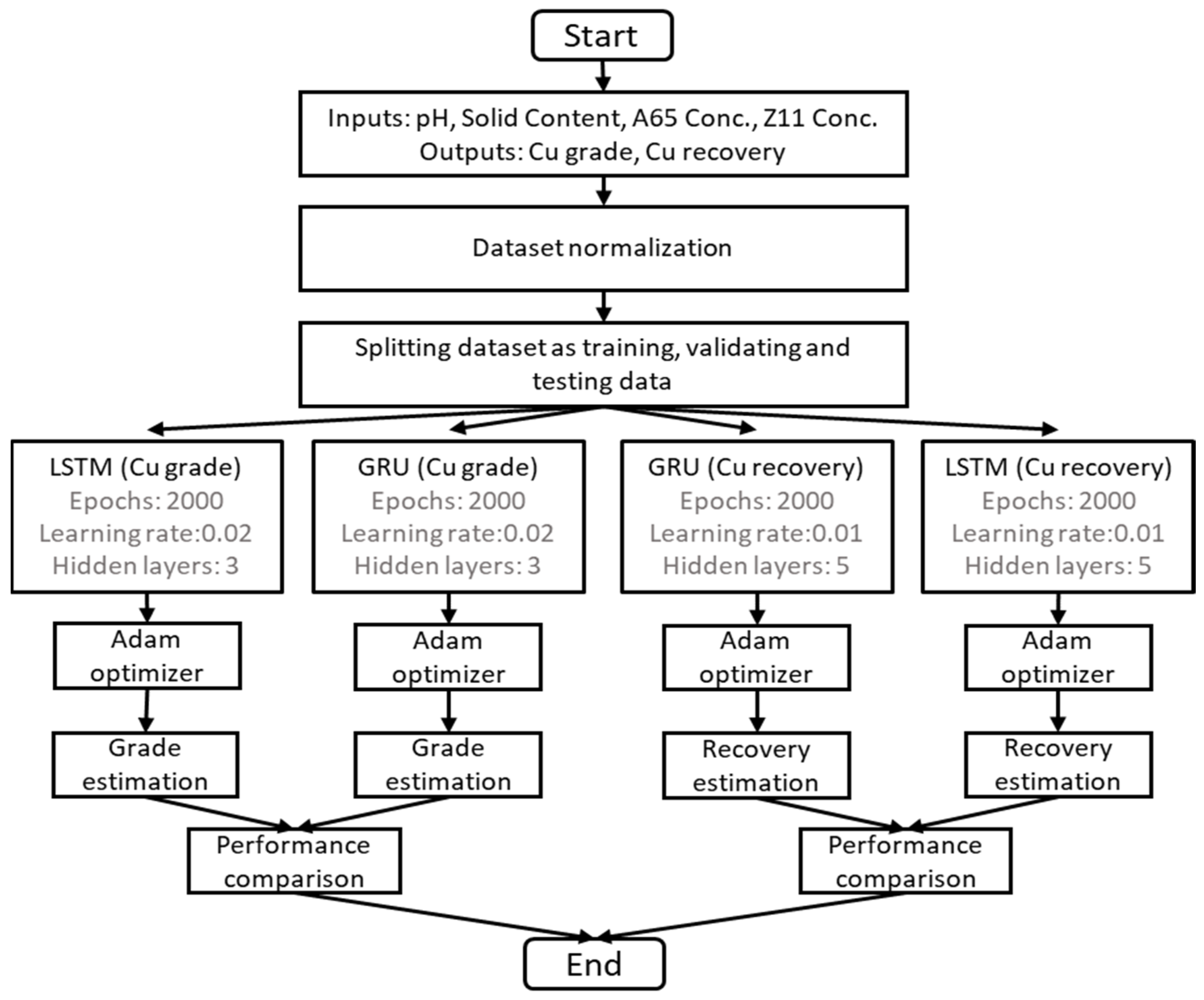
2.6. Recurrent Neural Network Simulation

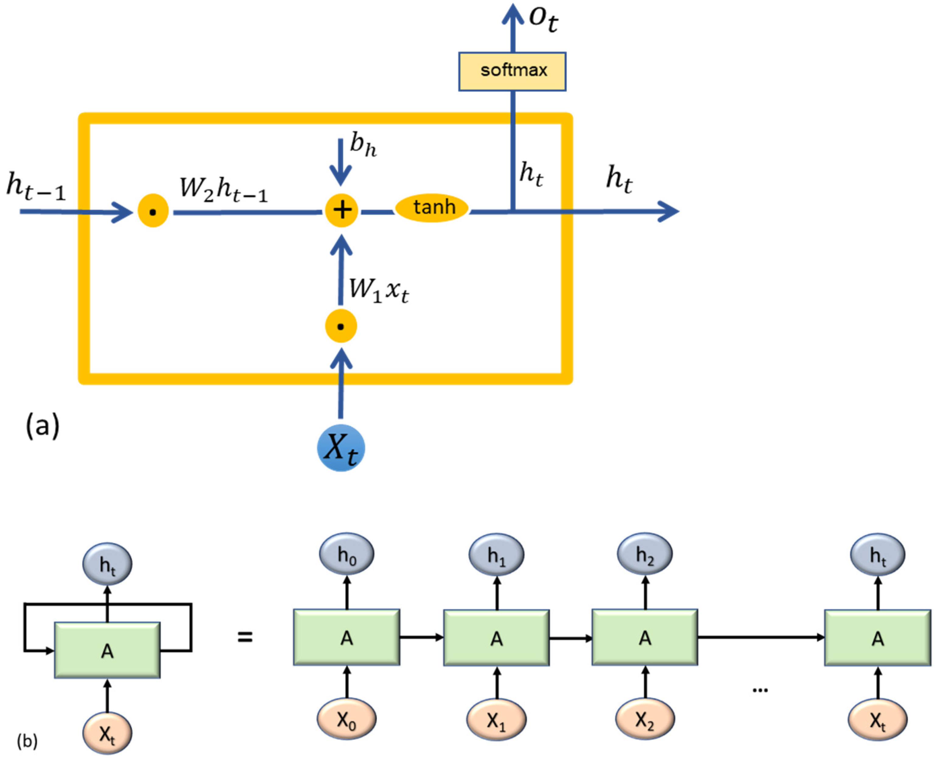
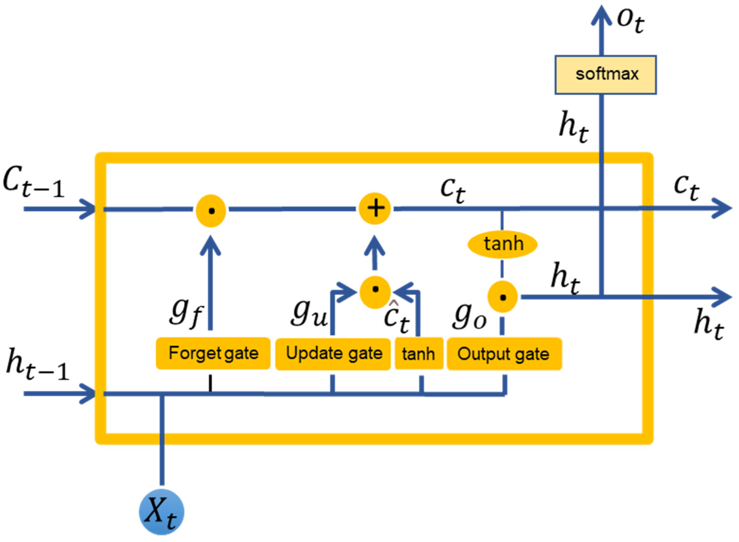
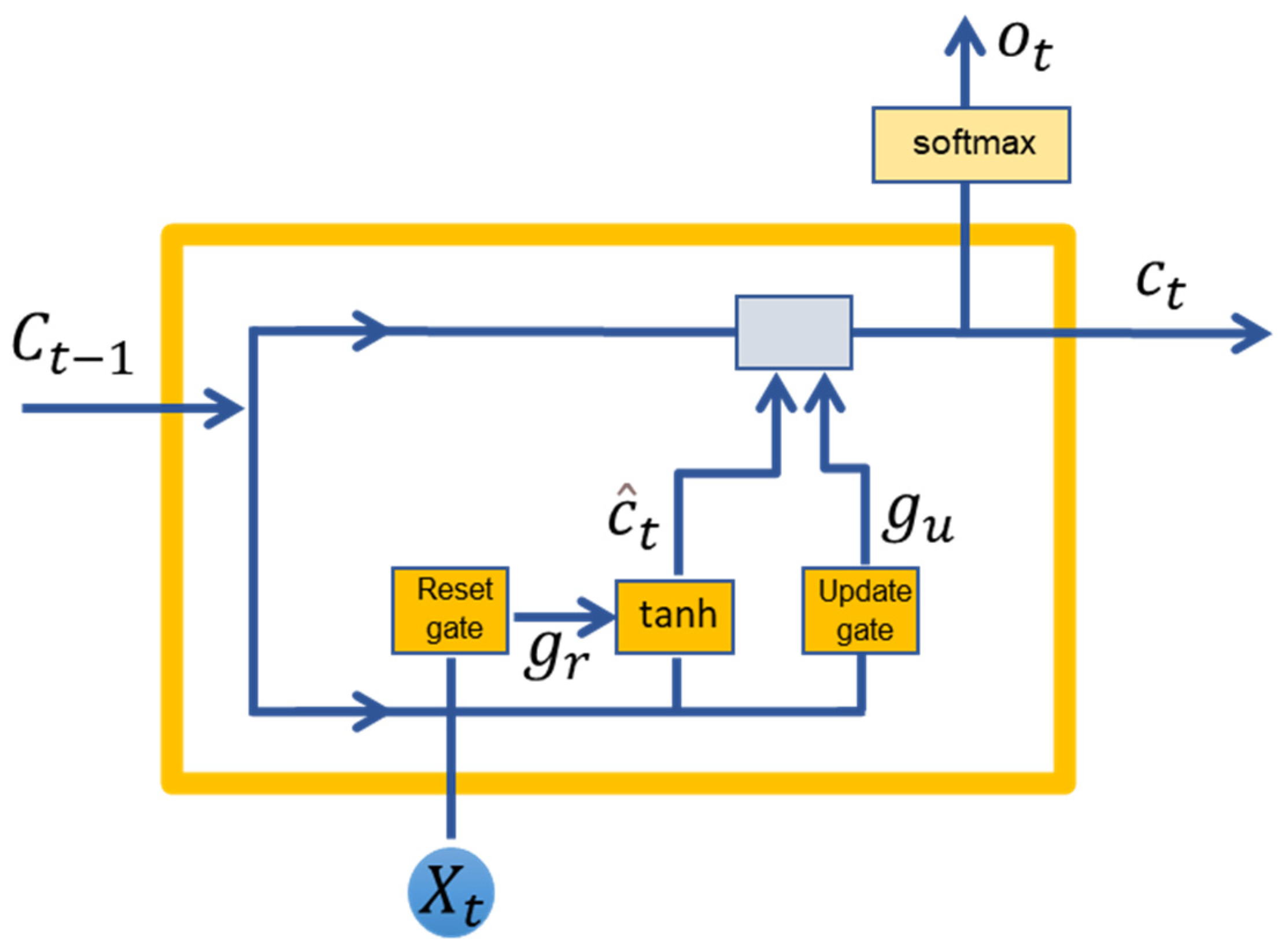
2.6.1. RNN-Based Methods

(A) Recurrent neural network: Since the long short-term memory (LSTM) and gated recurrent unit (GRU) networks are improved variants of the recurrent neural network (RNN) and are used in state-of-the-art deep learning applications, the structure of RNN was discussed first. The RNN is a type of feedforward neural network that maintains internal memory and is able to remember information throughout time. This property makes it proper for processing time series and sequential data [28]. The network structure and circuit diagram of RNN are shown in Figure 2.

In the circuit diagram, RNN takes X₀ from the input sequence and then delivers h₀ as the output, which together with X₁ are the inputs of the next step. Similarly, h₁ along with X₂ are the inputs to the next step, and so on. In such a manner, RNN constantly remembers the information during the training. The current state formula is as follows:

$$h_t=f\left(h_{t-1},x_t\right),$$

(2)

where x_t and h_t are the input and output sequence of a RNN unit, respectively. Equation (3) is also used to apply tanh as the activation function, which helps to regulate the values that flow through the network. Finally, y_t is the network output [29]:

$$h_t=\tanh \left(W_{hh}{h}_{t-1}+W_{xh}{x}_t\right),$$

(3)

$$y_t=W_{hy}{h}_t,$$

(4)

where W and h represent the weight and hidden vectors, respectively. W_hh is the weight in the previous hidden state, W_hx is the weight in the current input state, and W_hy represents the weight in the output state. tanh is an activation function that implements nonlinearity. Although RNN is theoretically designed to predict time series, it is difficult to predict long time series in practice because of the length of information, which can cause a vanishing gradient [30]. LSTM and GRU are the updated versions of RNN to overcome this challenge.

(B) Long short-term memory network (LSTM): LSTM is a special kind of RNN network that was introduced first by Hochreiter and Schmidhuber [31] and is able to tackle the problem of vanishing gradient and long length input processing of RNN. The LSTM network has internal mechanisms called gates. These gates (including input gates, forget gates, and output gates) control the data flow and also specify what data is important in the sequence and should be retained and what data should be removed. In this way, the network passes important information along the sequence chain to obtain the final output [32]. A structure diagram of LSTM is shown in Figure 3.

In Figure 3, x_t, h_t, and C_t are the input, the output, and the cell state at time t, respectively. g_f controls the information flow from the previous time step and is called the forget gate. This gate determines whether or not the information from the previous step is used. The update gate, which is indicated with g_u, is responsible for controlling the new information flow. This gate determines whether new information should be used at the current time step. g_o is the output gate and specifies how much of the previous information of time steps (previous and current) is transferred to the next time step. W, b, and σ are the weight of the model, the bias of the model and the activation function, respectively. The following equations represent the calculation process:

$${\widehat{C}}_t=\tanh \left(W_c·\left[h_{t-1},X_t\right]+b_c\right),$$

(5)

$$C_t=g_f·C_{t-1}+g_u·{\widehat{C}}_t,$$

(6)

$$g_f=\sigma \left(W_f·\left[h_{t-1},X_t\right]+b_f\right),$$

(7)

$$g_u=\sigma \left(W_u·\left[h_{t-1},X_t\right]+b_u\right),$$

(8)

$$g_o=\sigma \left(W_o·\left[h_{t-1},X_t\right]+b_o\right),$$

(9)

$$h_t=g_o·\tanh \left(C_t\right).$$

(10)

(C) Gated recurrent unit network (GRU): GRU was introduced by Chung et al. [33] to address the shortcomings of the traditional recurrent neural network and also to reduce the overload of LSTM architecture. The GRU has only two gates, including update and reset gates, compared with the LSTM. These gates are basically two vectors that are used to decide whether the information is transmitted to the output or not [34]. A structure diagram of GRU is shown in Figure 4 and relevant equations can be found below:

The reset gate specifies how much of the previous information is not needed (forgotten) and how much of the previous step information is used in the current step. The update gate specifies whether to use the previous state or current input (or a combination of both) at a time step. x_t is the input at time t, and σ is the activation function and h_t and h_t−1 are the output at time t and t − 1, respectively. The calculation process is expressed by the following equations:

$${\widehat{C}}_t=\tanh \left(W_1·\left[g_r·C_{t-1},X_t\right]+b_c\right),$$

(11)

$$g_u=\sigma \left(W_2·\left[C_{t-1},X_t\right]+b_u\right),$$

(12)

$$g_r=\sigma \left(W_3·\left[C_{t-1},X_t\right]+b_r\right),$$

(13)

$$C_t=g_u·{\widehat{C}}_t+\left(1-g_u\right)·C_{t-1}.$$

(14)

where g_r and g_u are the outputs of reset gate and update gate at time t.

2.6.2. Modelling Process

RNNs are considered the state-of-the-art algorithm for sequential data. LSTM and GRU are RNN-based algorithms that were developed with new designs to address the weaknesses of traditional RNNs. In this study, four inputs were included as pH, solid content (%, w/w), A65 concentration (g/t), and Z11 concentration (g/t); and the outputs were Cu grade (%) and its recovery (%). To analyse the methods and estimate outputs, four models were developed using the inputs. Table 4 shows the inputs and outputs as the operation factors and responses, respectively. Although controlling the flow of information is the same in both LSTM and GRU, LSTM wraps the hidden state into a memory unit, and GRU just passes the full hidden content without any control directly to the next cell. The models’ parameters, including number of hidden layers, number of epochs, etc., were carefully examined and selected based on the complexity of the data and trial and error procedure. Indeed, as a result of increasing the number of parameters, overfitting occurred. An overfitted model has high accuracy on training data but low accuracy on test data. For the number of epochs, increasing this parameter had no significant effect on the accuracy of the model; it only increased the time it took to develop the model. The optimal amounts of parameters were selected according to the mentioned points. In addition, the GRU and LSTM algorithms are similar in general structure, and the most important difference is that there are fewer parameters in GRU, which accounts for its faster training time. One of the purposes of using these two algorithms in this project, in addition to effectively predicting the outputs, is to examine the results of these two models in order to select a more appropriate algorithm. LSTM has a significant advantage over the GRU algorithm in accordance with its more complex structure. Figure 5 shows the flowchart of the modelling procedure to estimate the Cu grade and recovery using RNNs.

Random forest (RF) and ANN with the Levenberg–Marquardt optimization algorithm (ANN-LMA) as the two other popular prediction methods were also implemented for comparison:

• Random forest is a powerful learning method for classification and regression problems by constructing a multitude of decision trees at training time. This non-parametric method uses ensemble learning to avoid overfitting. To find the optimum number of trees, different numbers were tested. Based on the results, 26 and 22 trees were found to have the most accurate prediction for Cu grade and Cu recovery, respectively, and increasing the number of trees did not have significant impact on the accuracy of results. The optimum depth of the tree was also found to be 4 for both Cu grade and recovery models, and increasing the maximum depth of trees resulted in overfitting;
• LMA is known as the preferred method for minimization in nonlinear least squares problems. LMA interpolates between the Gauss–Newton algorithm and the gradient descent method. Compared with Gauss–Newton, Levenberg–Marquardt is more robust and, in many cases, it will find a solution even if it starts very far from the final minimum. ANN-LMA was found to be superior in Ref. [19] against other metaheuristic algorithms. The proper structure for ANN-LMA was found to be 5-12-4-1 for the Cu recovery model and 5-10-5-1 for the Cu grade model based on trial and error.

The coding and modelling process was implemented using MATLAB software (MathWorks R2021b v9.11, MathWorks, Inc., Natick, MA, USA). Before modelling, normalization was applied to improve the networks training phase using Equation (15) [12]:

$$x_n=\left(\frac{x_i-x_{min}}{x_{max}-x_{min}}\right),$$

(15)

where X_n and X_i are normalized and actual values, respectively. X_min and X_max are the minimum and maximum values of each subset (inputs–outputs). Besides the modelling process, the Spearman correlation analysis, to find out the relationship between inputs and outputs, and sensitivity analysis to calculate the effectiveness of each input data on the outputs were also applied; the outcomes are presented in the Section 3.

3. Results and Discussion

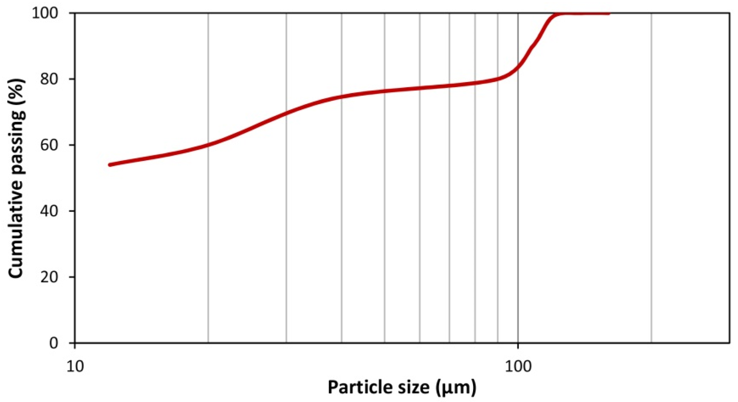
3.1. Results of Ore Characterization

The mineralogical results showed that chalcopyrite and chalcocite are the predominant copper-bearing minerals in the ore. The most important gangue minerals were pyrite and clay minerals. The particle size distribution of the studied ore sample is shown in Figure 6. The feed to the flotation circuit contains 80% by weight of particles finer than 78 µm.

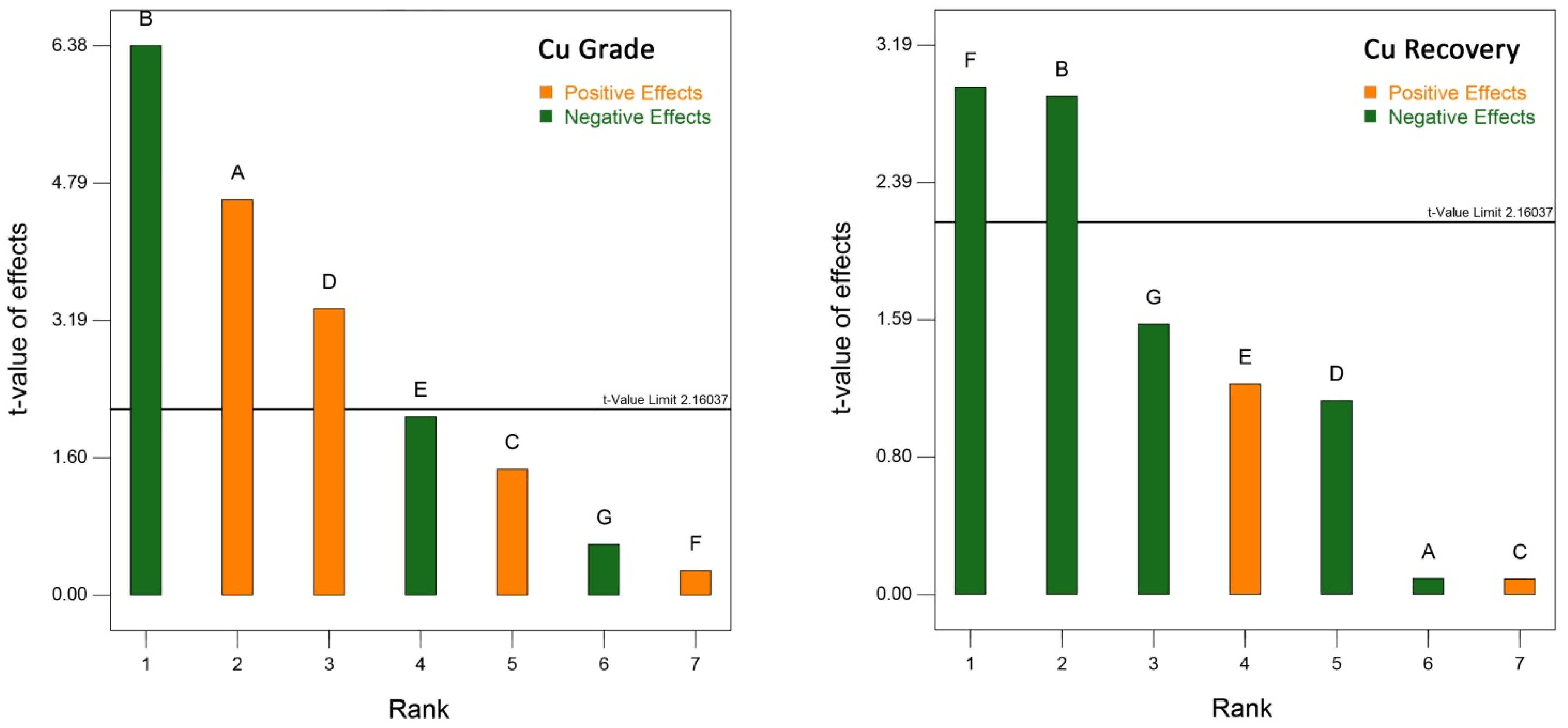
3.2. Statistical Analysis of Screening DOE

To determine the most important parameters affecting metallurgical responses, Pareto charts were drawn based on the results of variance analysis. Pareto charts are quick tools used to assess the significance level and the type of impact (increasing or decreasing) of the parameters under study. In these charts, effects with a value greater than t-value are identified as the significant factors. The type of effect is also shown by the software and based on the relevant statistical calculations with different colours. According to Pareto charts of grade and copper recovery in Figure 7, it can be seen that the most significant operating parameters affecting the grade of concentrate are solid percentage (B) > pH (A) > and concentration of A65 frother (C). Generally, the copper grade decreases significantly with the increasing solid content mainly due to transporting gangue minerals (i.e., pyrite, silicates and clay minerals) into the concentrate through the false flotation process [35]. This result is in line with the outcomes presented by previous studies [20,36]. Copper grade is also significantly affected by pH and A65 concentration. Although the effects of DTU (E) and MIBC (C) concentrations are relatively high, these effects are not statistically significant.

Although the solid content (B) and the concentration of Z11 (F) are the most effective factors affecting copper recovery, their effects are both negative. It should be noted that since the interaction effects of the parameters in factorial designs cannot be analysed due to bias, providing any physical interpretation for the main effects observed in these diagrams cannot be reliable. For this reason, the results of this design have only been used to select the most effective operational variables for detailed studies. In addition, according to the type of effect, the amount of levels considered in the optimization plan was also modified. For example, according to Figure 7, the effect of solid content on both responses is negative; therefore, the levels of this parameter in the screening design (20–30) were reduced in the optimization design i.e., 10–20, and similarly, the amount of levels was increased for the frother concentration and decreased for the collector concentration. The pH levels were not changed due to the operational limitations.

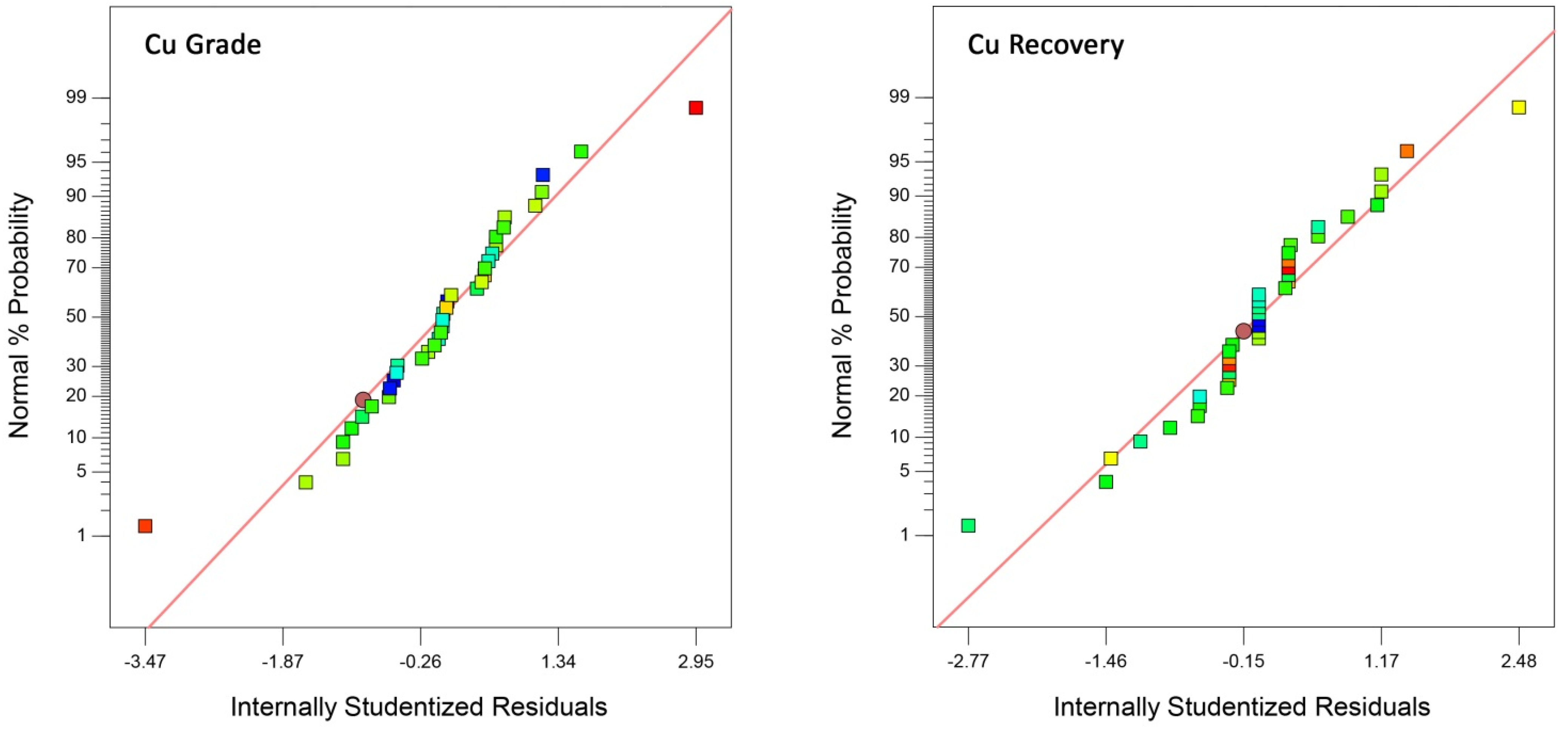
3.3. Statistical Analysis of Optimization DOE

The first step in analysing the impact of operational variables on the process responses is developing a parametric model that can accurately predict the desired response in the operating space, i.e., within the low to high levels intended for the variables [37]. In the second step, after developing the initial model by the software, abnormal data were identified by examining the model parameters and the model was optimized by the user to achieve the best fitting results. The result of these measures for the data obtained in the flotation experiments was the development of nonlinear models for all process responses as below:

$$\begin{array}{c}Cu Grade \left(\%\right)=10.17+0.35A+2.15B-0.39C-1.16D-0.65AB+0.46AC+1.30AD+0.24BC +\\ 0.62BD-0.17CD+0.54ACD-1.26BCD+0.68ABCD,\end{array}$$

(16)

$$\begin{array}{c}Cu Recovery \left(\%\right)=45.91+0.91A-0.72B+3.34C+0.28D-0.59AB-3.41AC-2.16BC+0.91BD +\\ 5.22CD+1.71ABC-0.97ABD-1.53ACD-1.78BCD-1.90ABCD,\end{array}$$

(17)

where the factors are described in a coded form. The validation parameters for the developed models are listed in

Table 5. Validation parameters showing the significance of the models for metallurgical responses.

Model	F-Value	p-Value	R2 (%)	Adj R2 (%)	Pred R2 (%)	Adeq Precision
Cu Grade	1251.23	<0.0001	99.86	99.78	99.57	134.99
Cu Recovery	24.07	<0.0001	94.50	90.58	88.62	20.59

. According to Fisher’s F-test and marginal probability value (p model < 0.0001), which are shown in Table 5, all of the suggested prediction models are significant. For assessing the significance of a predictive model, the residuals normal probability plot is an effective tool [38]. According to the normal probability plots shown in Figure 8, all responses were relatively uniform, confirming the assumptions of normality and the independent nature of residuals during the statistical analyses. In addition, the high values of the adjusted correlation coefficients also indicate the significance of the prediction models. The Pred R² values were reasonably high, indicating that the model is able to explain variability in the prediction of new observations with adequate accuracy, which is in reasonable agreement with the Adj R² values [39]. Another statistical measure, called adeq precision, shows the signal-to-noise ratio, and any value over 4 is considered desirable [6]. In this investigation, the ratios were 134.99 and 20.59 for copper grade and recovery, respectively. These values show an adequate signal so that the models can be used to navigate the design space and predict appropriately.

Model Equations (16) and (17) were used to assess the significance of operating variables on process responses.

Table 6. Analysis of variance results for copper grade to the rougher concentrate.

Source	Sum of Squares	df	Mean Square	F-Value	p-Value (Prob > F)
Model	363.8967	13	27.99206	1251.234	<0.0001
A-pH	3.822613	1	3.822613	170.8693	<0.0001
B-Solid Content	147.3186	1	147.3186	6585.085	<0.0001
C-A65	4.8672	1	4.8672	217.562	<0.0001
D-Z11	43.29151	1	43.29151	1935.114	<0.0001
AB	13.4162	1	13.4162	599.699	<0.0001
AC	6.826513	1	6.826513	305.1425	<0.0001
AD	54.2882	1	54.2882	2426.662	<0.0001
BC	1.814513	1	1.814513	81.10801	<0.0001
BD	12.5	1	12.5	558.7452	<0.0001
CD	0.973012	1	0.973012	43.49328	<0.0001
ACD	9.46125	1	9.46125	422.9142	<0.0001
BCD	50.6018	1	50.6018	2261.881	<0.0001
ABCD	14.71531	1	14.71531	657.7688	<0.0001
Pure Error	0.485733	21	0.02313
Cor Total	367.9095	37

and

Table 7. Analysis of variance results for copper recovery to the rougher concentrate.

Source	Sum of Squares	df	Mean Square	F-Value	p-Value (Prob > F)
Model	2266.4	15	151.0933	24.07371	<0.0001
A-pH	31.7761	1	31.7761	10.309121	0.0043
B-Solid Content	35.5092	1	35.5092	12.092561	0.0031
C-A65	356.5785	1	356.5785	56.81369	<0.0001
D-Z11	44.2345	1	44.2345	14.291302	0.0021
AB	11.3288	1	11.3288	1.805019	0.1934
AC	372.5085	1	372.5085	59.35182	<0.0001
AD	16.4738	1	16.4738	2.624772	0.1201
BC	149.5585	1	149.5585	23.82917	<0.0001
BD	26.3538	1	26.3538	4.198954	0.0531
CD	873.411	1	873.411	139.1607	<0.0001
ABC	93.91351	1	93.91351	14.96325	0.0009
ABD	29.9538	1	29.9538	4.772542	0.0404
ACD	74.48101	1	74.48101	11.86707	0.0024
BCD	100.891	1	100.891	16.07498	0.0006
ABCD	115.596	1	115.596	18.41792	0.0003
Pure Error	131.8018	21	6.276278
Cor Total	2408.51	37

show the ANOVA results within a confidence interval of 95%. As shown in Table 6 and Table 7, the effects of all operational variables on process responses are statistically meaningful due to p-values less than 0.05. As seen in the analysis of variance tables, no interaction was considered in the analyses. Moreover, except in some cases for the copper recovery analysis, the dual interaction effects are significant. The statistically meaningless interactions for copper recovery are those between pH and solid content and Z11 concentration as well as the interaction between solid content and Z11 concentration.

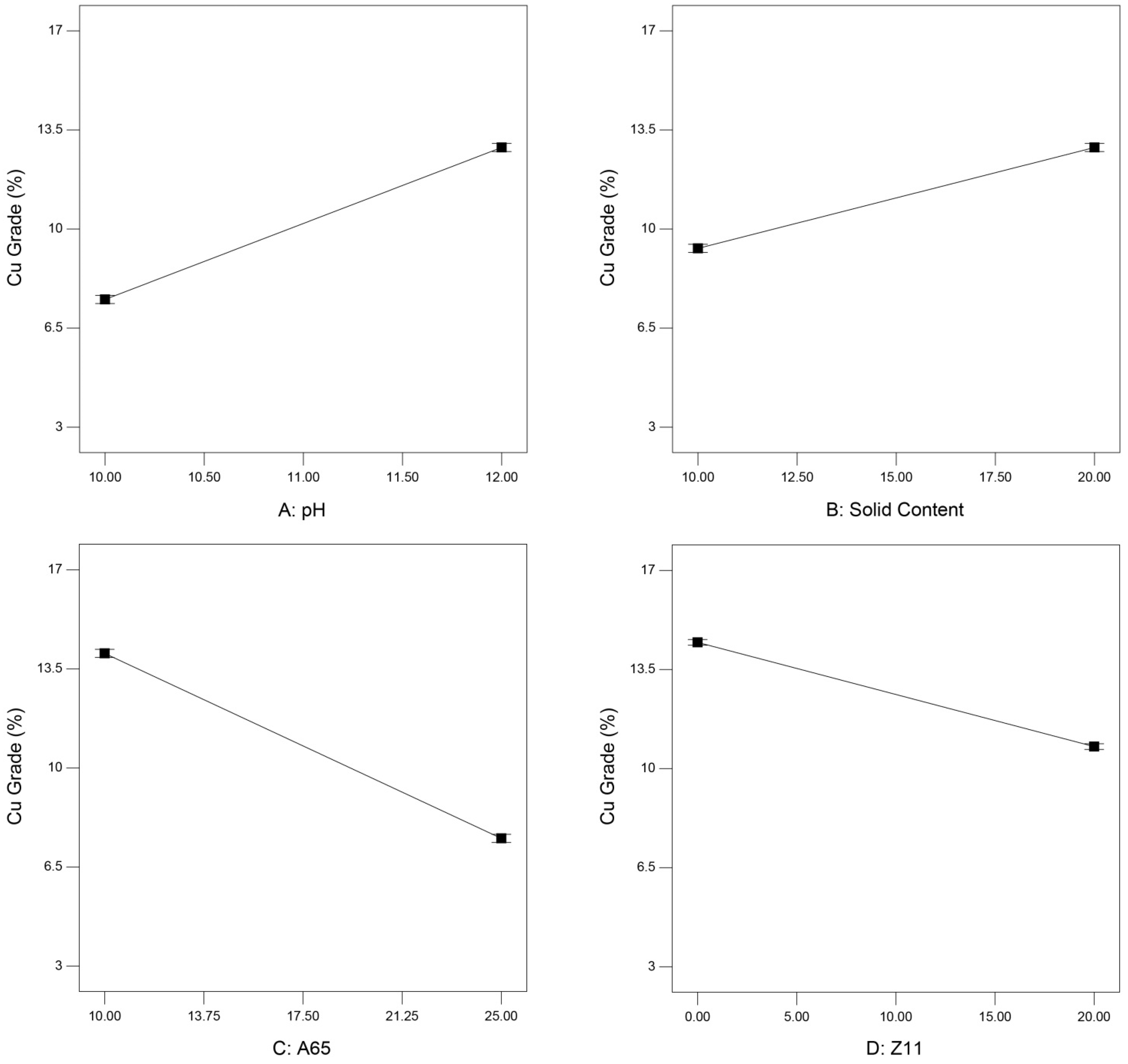
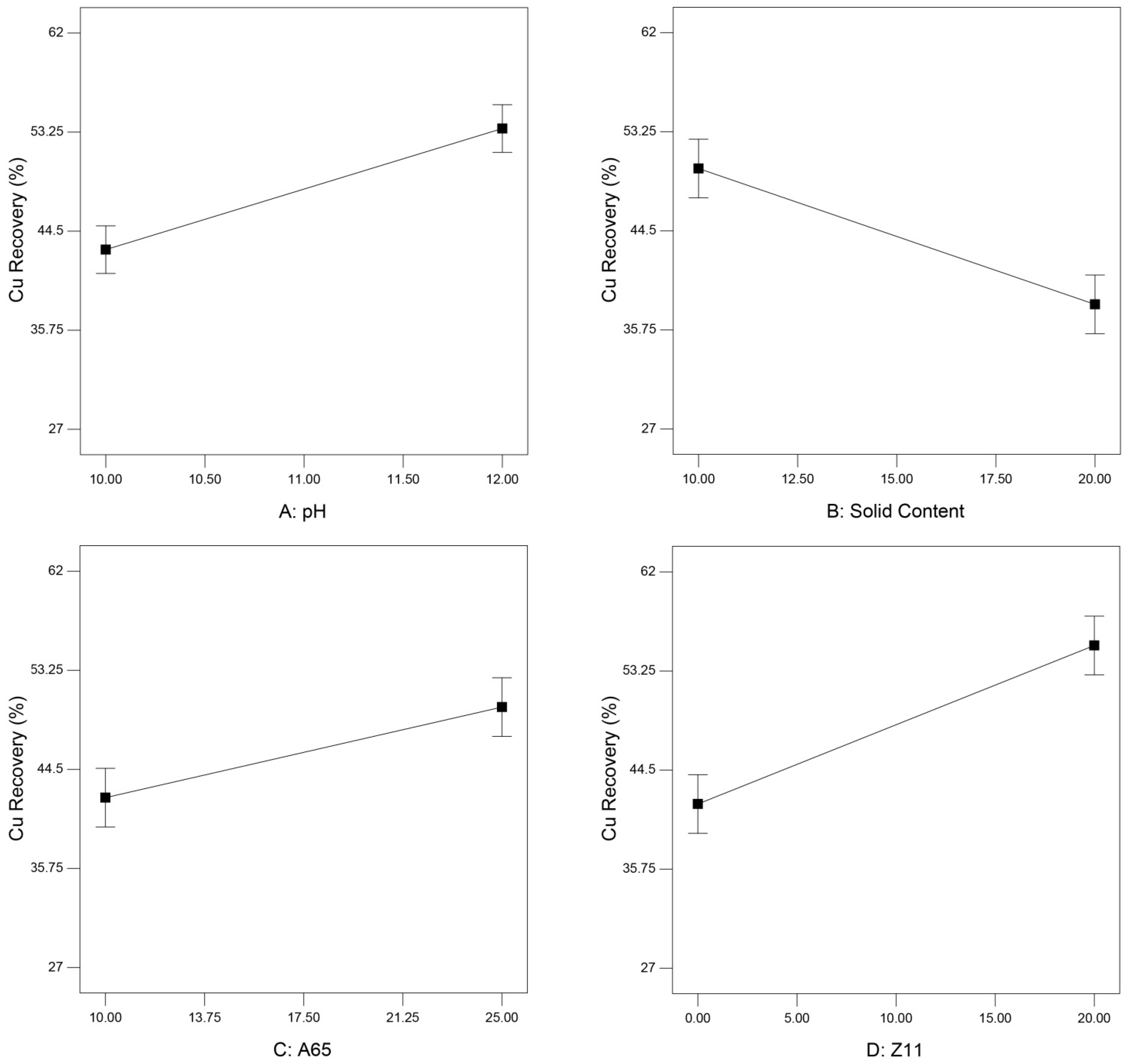
3.3.1. Interpretation of the Main Effects

The main effect plots can be used to analyse the effects of the operating variables on the process response. These plots are an effective tool for assessing the influence of each variable on the target response. The response variation is shown in these plots for the level of variables used in the experimental design. Design Expert software uses, by default, the developed prediction model (Equations (16) and (17)) to calculate the response values for parameters varying within their experimental levels. In contrast, other variables are maintained at their mid-levels. The main effects plots of different operating variables are shown in Figure 9 and Figure 10 for copper grade and recovery, respectively.

According to Figure 9, the copper grade increases with the increasing pH. Obviously, as the pH increases, the pyrite depression rate also increases, and as a result, the copper grade in the concentrate improves. The effect of increasing the solid content on copper grade is also positive and increasing. This effect can be attributed to the improved particle distribution within the flotation cells, thereby increasing the probability of copper-containing particles colliding with the bubbles and transporting them to the froth and concentrate. However, as shown in Figure 10, copper recovery decreased with the increasing solid content, which can be ascribed to the interaction between the solid content and the frother concentration, as will be discussed later. Increasing the concentration of both frother and collector reduces the grade of copper in the concentrate. With an increasing frother concentration, due to increased bubble stability and increasing the rate of bubbly regime in the pulp zone, the entrainment rate will most likely increase due to the swarm phenomenon, and finally, the copper grade decreases as a consequence of the gangue particles transfer to the concentrate [40,41]. The effect of increasing the collector concentration is also due to the increase of hydrophobicity level and floatability of gangue minerals and, as a result, their transfer to the concentrate. Therefore, the copper grade in concentrate is expected to decrease. These phenomena, namely the increase in entrainment rate and the improvement of gangue floatability, will increase the solid transfer rate into the concentrate and, consequently, increase the recovery; this prediction is clearly seen in Figure 10.

Increasing the pH, in addition to improving the grade of copper, has also increased the recovery (Figure 10). As the pH increases, the efficiency of the xanthate collectors (Z11 in this study) improves, resulting in increased particles floatability. For this reason, particle recovery is also expected to improve. The negative effect of solid content on the recovery can be evaluated according to the interaction of this factor with the frother concentration, which is presented in Section 3.3.2. Given that the main effect plot for each factor is plotted while other factors are kept constant at their mid-level, the individual effect of the solid content may lead to the misleading conclusion that increasing the solid content in any condition causes reduction, leading to recovery.

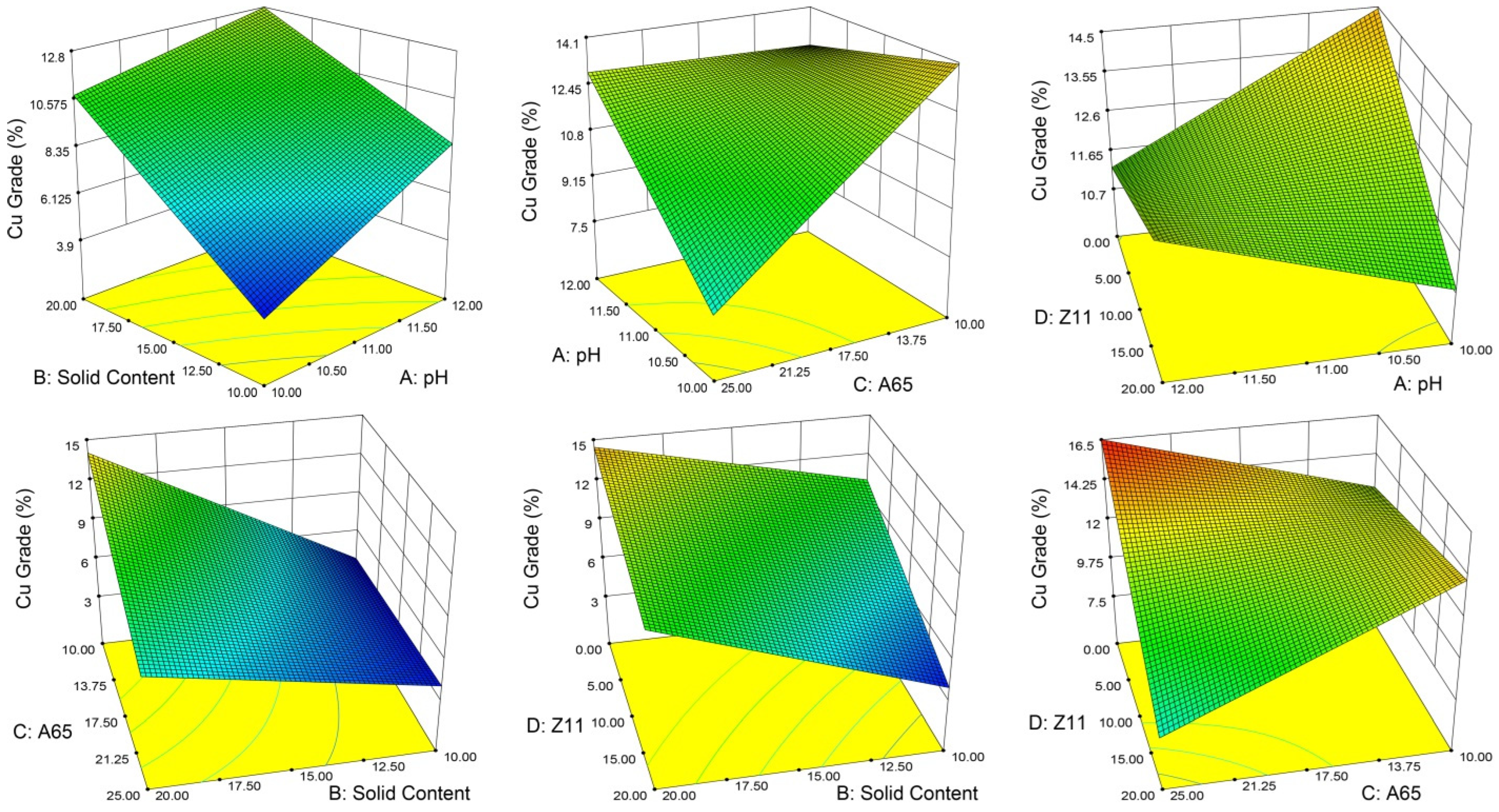
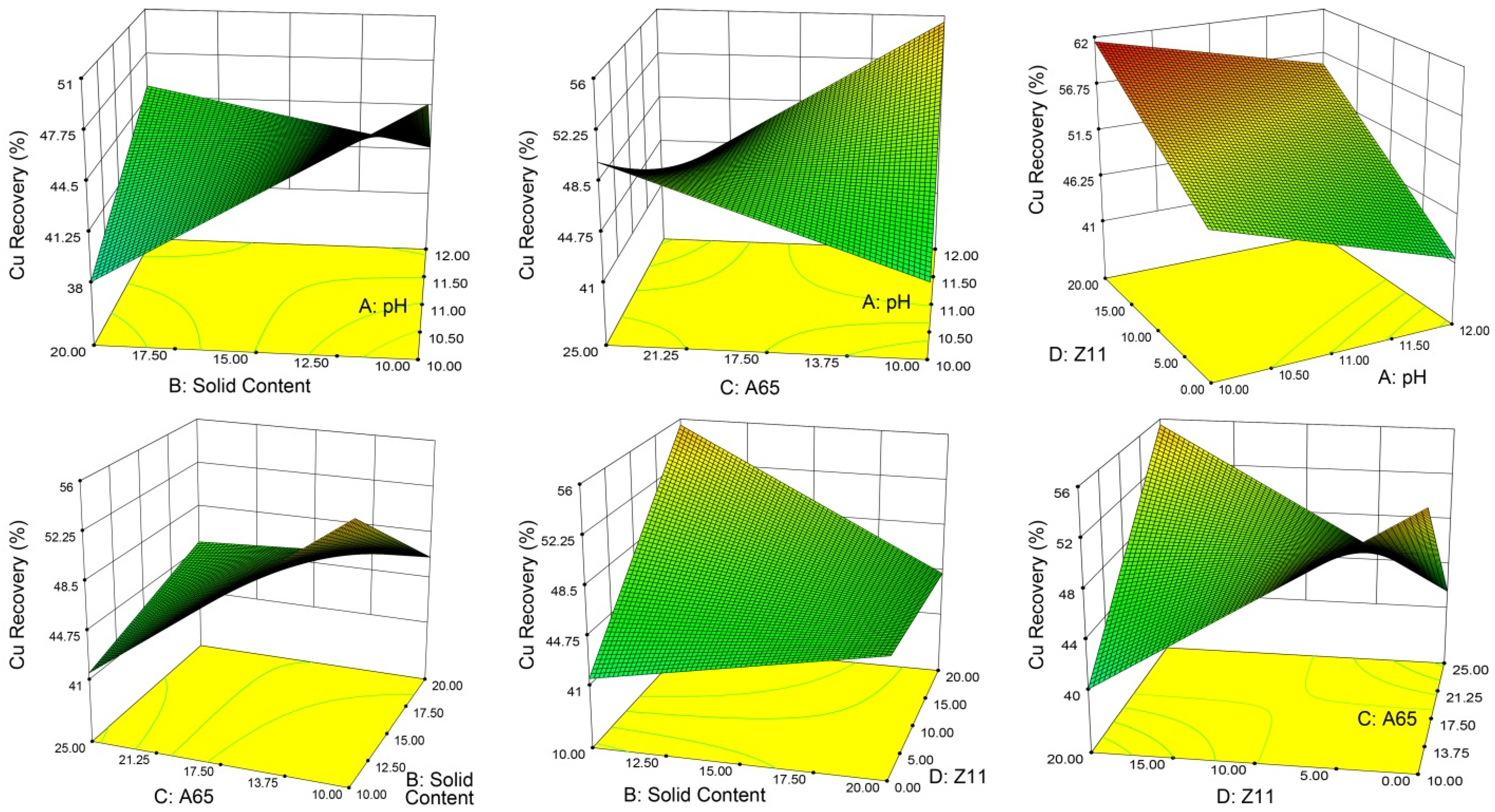
3.3.2. Evaluation of the Interactive Effects

The surface plots of the response of a process against other independent variables can provide valuable insights into not only the individual effect of operating factors, but the potential interaction between them as well [42,43]. Thus, the surface plots for the studied flotation experiments were presented. As shown in Figure 11 and Figure 12, the surface response plots illustrate the nonlinear effects of most interactions among four variables. As mentioned earlier, the interaction between solid content and frother concentration (Figure 12) shows that maximum copper recovery can be obtained at a low level of frother concentration, whereas individual effects yielded contrary results. This conclusion can be directly attributed to the significant interaction between those variables. Due to this effect, it seems that the balance between the amount of particles in the system and the number of stable bubbles plays a significant role in improving the process efficiency. The same behaviours are observed for copper grade, as it may be concluded that the highest copper grade can be achieved at a high level for pH and solid content and a low level for reagents dosages when referring to the main effect plots. However, Figure 11 clearly shows different results. Similar results are observed in the case of copper recovery when evaluating the interactions given in Figure 12.

3.3.3. Process Optimization and Verification Studies

Maximum Cu grade and recovery were separately defined as target responses to find suitable operating conditions for each case. The operating conditions and the predicted results suggested by the software are given in

Table 8. The predicted and practical results for copper grade and recovery under optimal conditions.

Goal (Max)	pH	Solid Content (%)	A65 Conc. (g/t)	Z11 Conc. (g/t)	Predicted Responses (%)		Practical Results (%)
					G.	R.	G.	R.
Grade (G)	10.00	20.00	25.00	0.14	16.44	38.41	15.32	34.03
Recovery (R)	10.00	19.93	25.00	9.91	12.00	47.72	11.48	44.39

. To assess the accuracy of the predictions in Table 8, the plant was permitted to operate for 10 days under the suggested operating conditions and the metallurgical responses were monitored by regular sampling from each operating shift. Finally, an average value was reported as the final practical result, as given in Table 8. Compared to the grade values, the higher differences between the practical recovery results and predicted values are due to the lower accuracy of the prediction model developed by the software (Table 5).

3.4. Simulation Results

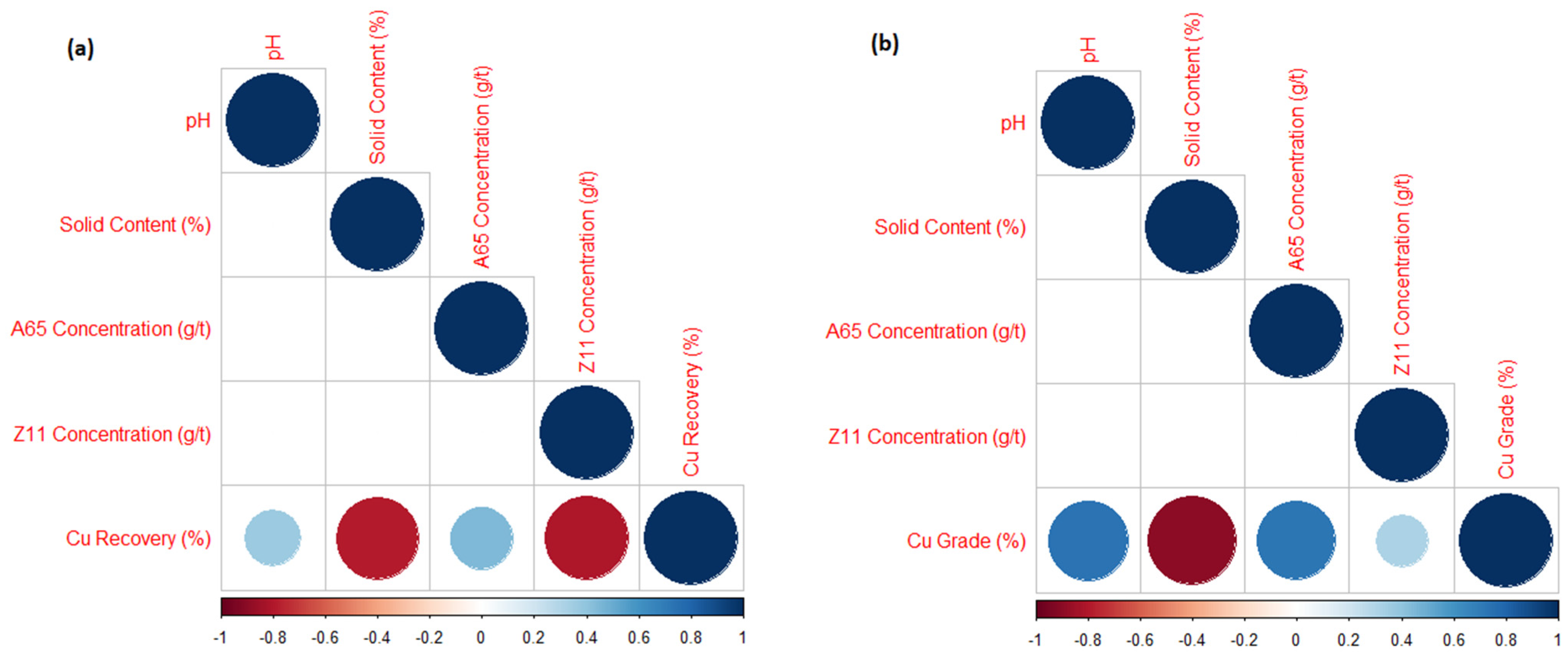
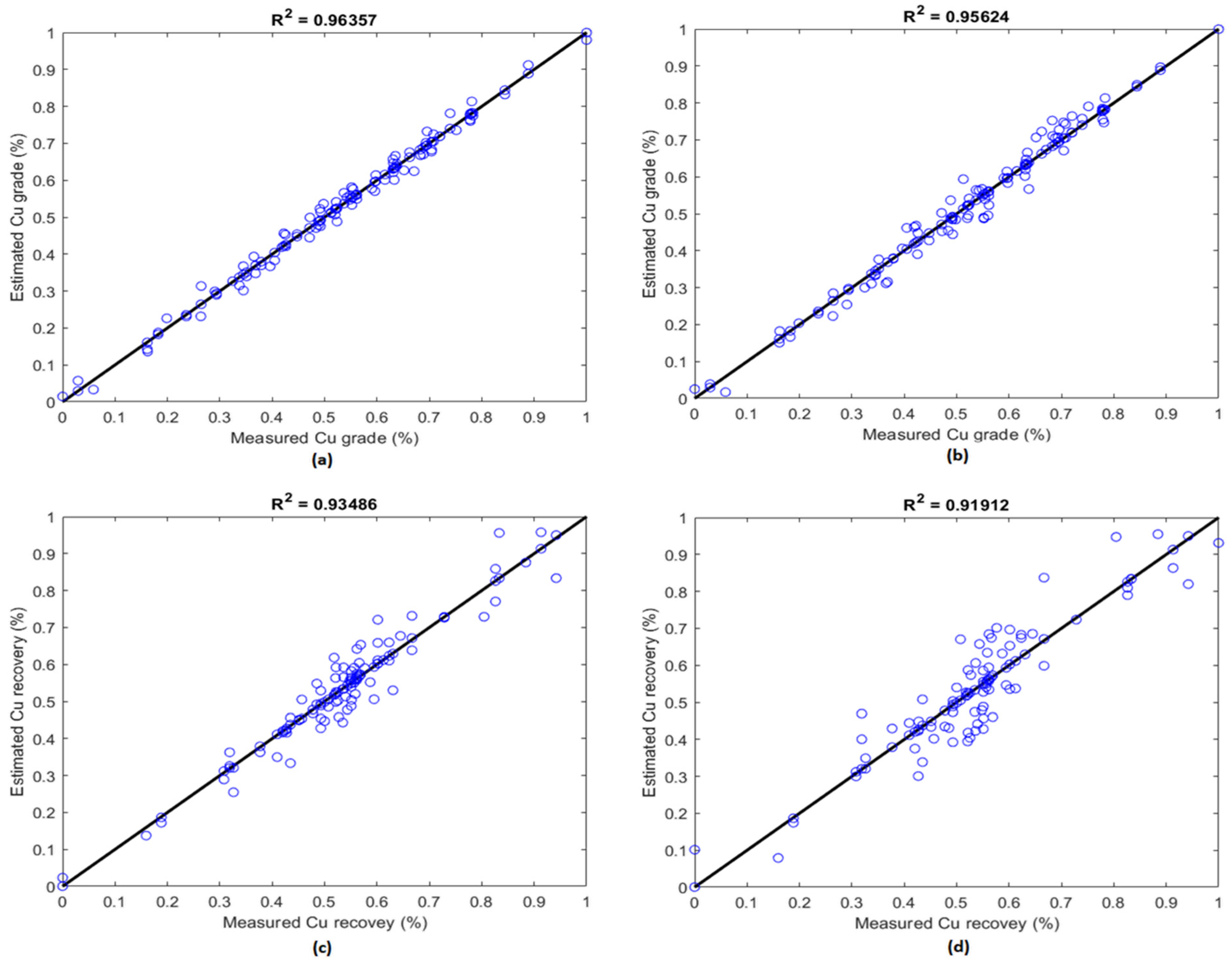
3.4.1. Correlation Coefficient Analysis

Correlation coefficient is an indicator that is used to measure the dependence or relationship between two variables. The correlation coefficient between each variable and the outputs (Cu grade and Cu recovery) confirms the existence of correlation. In this study, the Spearman correlation coefficient was used, which is defined as Equation (18) [44]:

$$\rho =1-\frac{6\sum d_i^2}{n\left(n^2-1\right)},$$

(18)

where ρ is Spearman’s rank correlation coefficient, d_i is the difference between the two ranks of each variable, and n is the number of samples. The correlation coefficient between each variable and the outputs is presented in Figure 13 and

Table 9. The correlation coefficient of the variables with Cu grade and Cu recovery.

Variable	pH	Solid Content (%)	A65 Conc. (g/t)	Z11 Conc. (g/t)
Cu grade (%)	0.7391	−0.8936	0.7234	0.3155
Cu recovery (%)	0.3653	−0.7880	0.4490	−0.8041

. The coefficients indicate that the variables had a good correlation and could be used to estimate Cu grade and Cu recovery.

According to Table 9 and for this study, pH and A65 concentration had a good positive correlation with Cu grade; on the contrary, the solid content had a strong negative effect on Cu grade. It means that should the pH increase, the Cu grade decreases, as was also reported in Ref. [45]. For the Cu recovery, Z11 concentration and solid content had high negative correlation with this output, and pH and A65 concentration had positive correlation, although their correlation coefficient is lower than 0.5. It is important to note that in the correlation coefficient methods, the closer the coefficient is to 1 and −1, indicates a direct or inverse relationship between the two variables. However, a cause-and-effect relationship is not necessarily present, and the conclusion cannot be drawn on this basis.

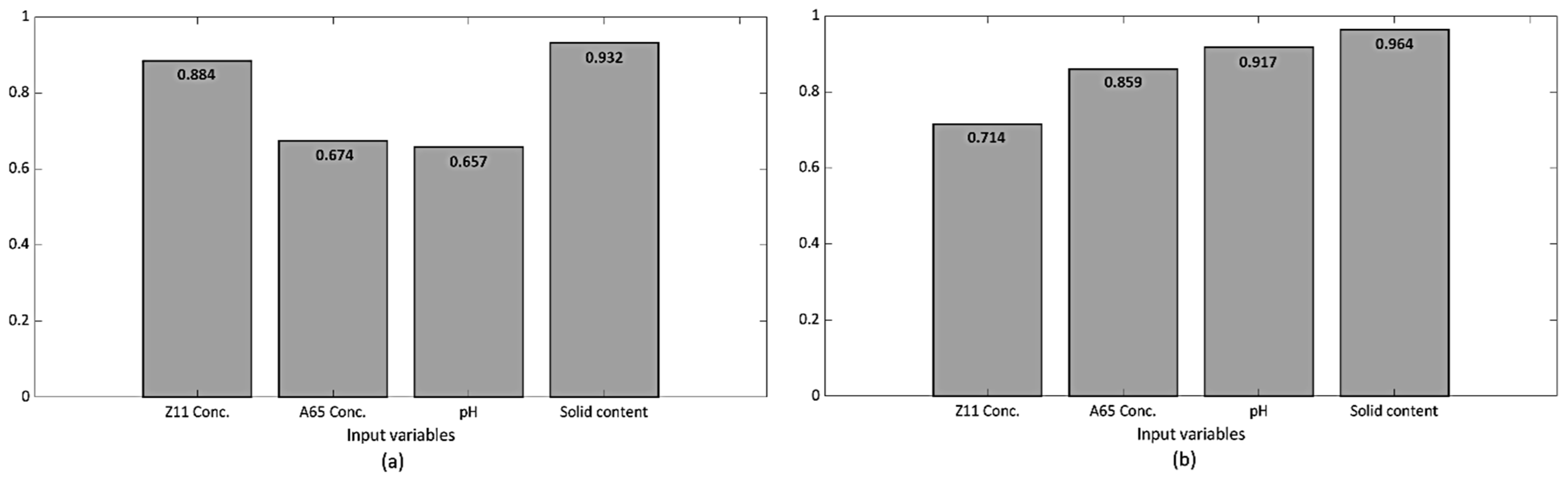
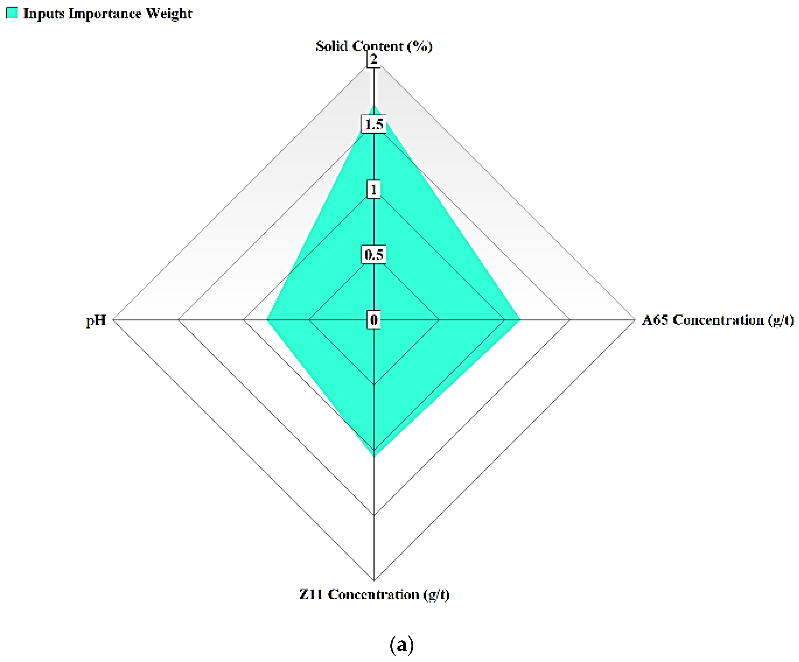
3.4.2. Sensitivity Analysis

In order to determine the effect of each input on the amount of output, a sensitivity analysis was also applied. In this paper, the input parameters were pH, solid content, A65 concentration, and Z11 concentration, and output parameters were Cu recovery and Cu grade. To calculate the sensitivity analysis, the following equation was used [46]:

$$R_{ij}=\frac{{{\displaystyle \sum }}_{k=1}^n\left(x_{ik}\times x_{jk}\right)}{\sqrt{{{\displaystyle \sum }}_{k=1}^n{x}_{ik}^2{{\displaystyle \sum }}_{k=1}^n{x}_{jk}^2}},$$

(19)

where x_i and x_j are the input and output datasets, respectively. The effect of each input parameter on the outputs is shown in Figure 14.

It can be seen in the figure that the solid content influenced both Cu recovery and grade the most. The results also confirm the correlation results to a great extent. Using the results of different tests, the variables that had a greater impact on the outputs were selected, which ultimately led to simulation models with greater accuracy and less error.

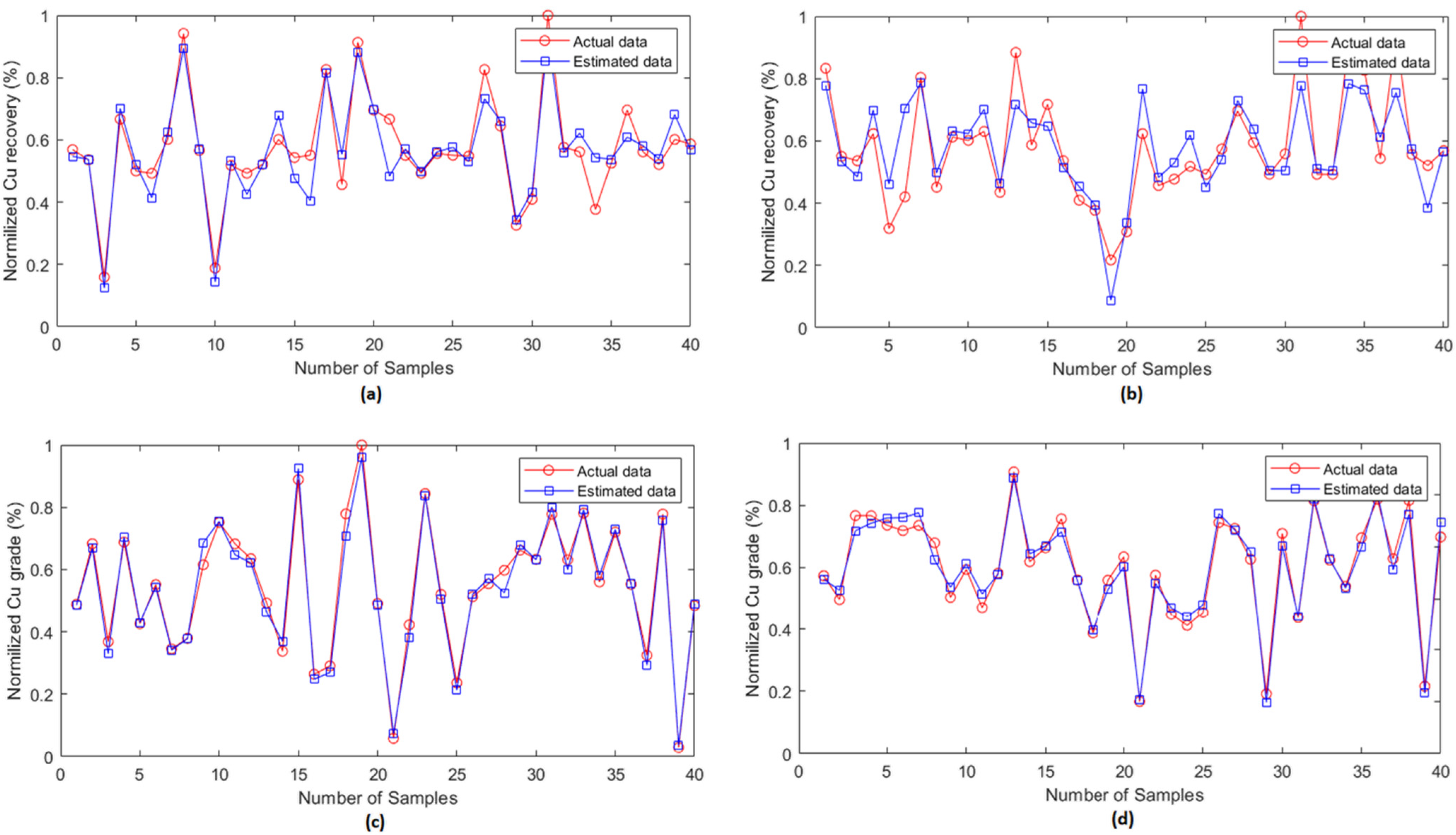
3.4.3. Model Prediction Analysis

The dataset was divided into three categories, including training (65%), validating (15%), and testing (20%). The validation dataset helps to tune hyper-parameters during the training of the models to prevent the models from over-fitting in the testing phase. The test performance of the ‘RNNs’ models is shown in Figure 15 and Figure 16.

Mean square error (MSE), root mean square error (RMSE), mean absolute percentage error (MAPE), and R² were computed using the following equations in order to evaluate the performance of each model [43,44]:

$$MSE=\frac{1}{n}{{\displaystyle \sum }}_{i=1}^n{\left(y_i-{\widehat{y}}_i\right)}^2,$$

(20)

$$RMSE=\sqrt{\frac{1}{n}{{\displaystyle \sum }}_{i=1}^n{\left(y_i-{\widehat{y}}_i\right)}^2},$$

(21)

$$MAPE=\frac{1}{N}{{\displaystyle \sum }}_{i=1}^N\frac{\left|{\widehat{y}}_i-y_i\right|}{{\widehat{y}}_i},$$

(22)

$$R^2={\left(\frac{{{\displaystyle \sum }}_{i=1}^N\left(y_i-\overline{a}\right)\left({\widehat{y}}_i-\overline{e}\right)}{\sqrt{{{\displaystyle \sum }}_{i=1}^N{\left(y_i-\overline{a}\right)}^2}\sqrt{{{\displaystyle \sum }}_{i=1}^N{\left({\widehat{y}}_i-\overline{e}\right)}^2}}\right)}^2,$$

(23)

where $y$ is the actual data, $\widehat{y}$ is the estimated data, $\overline{a}$ is the mean of actual data, $\overline{e}$ is the mean of the estimated data, and N is the number of sample sets.

The performance of the LSTM, GRU, RF, and ANN-LMA models in predicting Cu grade and its recovery is shown in

Table 10. Performance of the models to estimate Cu grade.

Model	MSE	RMSE	MAPE	R2
LSTM	5.5 × 10−3	0.074	5.7 × 10−5	0.963
GRU	8.7 × 10−3	0.093	6.3 × 10−5	0.956
RF	9.8 × 10−3	0.098	7.4 × 10−5	0.939
ANN-LMA	1.3 × 10−2	0.114	8.6 × 10−5	0.921

and

Table 11. Performance of the models to estimate Cu recovery.

Model	MSE	RMSE	MAPE	R2
LSTM	0.017	0.132	7.8 × 10−5	0.934
GRU	0.026	0.162	9.6 × 10−5	0.919
RF	0.028	0.167	1.1 × 10−4	0.915
ANN-LMA	0.029	0.170	1.3 × 10−4	0.914

. Based on the results, the performance of the RNNs is better than the other models; however, in the estimation of Cu recovery, the RF and ANN-LMA results are so close to the GRU. The RNN results are also close to each other (LSTM provides better accuracy). Although RF has a better result than ANN-LMA due to its tree structure in Cu grade estimation, when there are many calculations, a large number of trees can make the algorithm too slow and ineffective for real-time predictions. Both GRU and LSTM could validly estimate Cu grade and recovery. The results demonstrate that LSTM and GRU are useful deep networks for predicting time series and sequential data.

Although the accuracy of the RNN models is close, the number of parameters and time efficiency of the algorithms should be considered in practical applications [47,48]. The study showed that GRU performed faster with less CPU usage because it has fewer parameters for training. LSTM is more sophisticated and provides more parameters such as the number of weight matrices, number of bias vectors, learning rates, etc. This can be considered as a penalty for such models, as described in detail by Hassanzadeh et al. [49]. A model’s learning rate controls how quickly it can adapt to a new problem and is a crucial parameter for efficient training [29]. Larger learning rates result in rapid changes and require fewer training epochs; however, smaller learning rates allow the model to learn a more optimal set of weights, but may take significantly longer to train. The structure of GRU is more straightforward. It has one gate less than LSTM, which reduces matrix multiplication, and it can save time. However, through empirical research and as reported by Cahuantzi et al. [50] and Yang et al. [51], the advantage of GRU is only relevant for small datasets and when you have little memory. In other scenarios, when dealing with more extensive sequences, LSTM is preferred. Generally, it can be concluded that if the dataset is small, the GRU algorithm is preferable, whereas LSTM is favourable and more accurate for larger datasets. Furthermore, parameter optimization for the purpose of studying the influence of different setting parameters on these networks could be investigated in future research. To find insights on the structure of the estimation models, the importance and impact of each input variable on the outputs should be specified. The model estimation error was calculated when input values were randomly shuffled in order to assess the features importance. It is expected that permutation will increase the model’s estimation error if the model relies on an input value for estimation. Due to the superior performance of LSTM models for Cu grade and recovery, this process was applied to LSTM models and the results are shown in Figure 17. Features importance results are well aligned with results obtained through the Spearman correlation and sensitivity analysis. Besides, LSTM’s success in developing models and extracting meaningful characteristics from training data can also be confirmed by the results of feature importance and statistical analysis (Section 3.2).

4. Conclusions

The metallurgical response of a copper processing plant was predicted using two efficient variants of the recurrent neural network (RNN) method based on the effective operating parameters, including pulp pH and solid content as well as the concentrations of the frother and collector. For this purpose, the process was first evaluated using a two-step screening/optimization DOE based on factorial designs. Statistical results based on analysis of variance showed that there is a reliable correlation between the metallurgical responses, i.e., copper grade and recovery in concentrate, and operating variables. ANOVA results indicated that all operating variables significantly affect the metallurgical responses, such that the copper grade increased by increasing the pulp pH and solid content and decreased as the dosage of frother and collector were increased. Contrary results were observed with respect to the copper recovery, with the exception that, like grade, copper recovery increased with the increase of pulp pH due to interaction effect with other factors.

Afterwards, the optimization process was performed based on the identified significant factors and by applying particular adjustment in terms of the technical aspects of the process. The effect of the studied variables was also interpreted based on the main and interaction effects to obtain a meaningful vision for the simulation step. The correlation coefficient, mean, root mean square, and mean absolute percentage errors as well as variance account for values for the training and testing datasets for the copper grade and recovery using the long short-term memory (LSTM), and gated recurrent unit (GRU) networks were compared. The results showed that the LSTM algorithm was more efficient than the GRU network and can be applied to predict the metallurgical responses during the flotation process.

References

1. Adams, M.D. Advances in Gold Ore Processing; Elsevier: Amsterdam, The Netherlands, 2005. [Google Scholar]
2. King, R.P. Modeling & Simulation of Mineral Processing Systems; Butterworth-Heinmann: Boston, MA, USA, 2012. [Google Scholar]
3. Scharnhorst, A.; Börner, K.; van der Besselaar, P. Models of Science Dynamics; Springer: Berlin, Germany, 2012. [Google Scholar]
4. Kuhn, M.; Johnson, K. Applied Predictive Modeling; Springer: Berlin, Germany, 2018. [Google Scholar]
5. Herrell, F.E. Regression Modeling Strategies; Springer: Berlin, Germany, 2016. [Google Scholar]
6. Montgomery, D.C. Design and Analysis of Experiments, 10th ed.; Wiley: Hoboken, NJ, USA, 2020. [Google Scholar]
7. Asadi, E.; Isazadeh, M.; Samadianfard, S.; Ramli, M.F.; Mosavi, A.; Nabipour, N.; Shamshirband, S.; Hajnal, E.; Chau, K. Groundwater quality assessment for sustainable drinking and irrigation. Sustainability 2020, 12, 177. [Google Scholar] [CrossRef] [Green Version]
8. Shamshirband, S.; Hashemi, S.; Salimi, H.; Samadianfard, S.; Asadi, E.; Shadkani, S.; Kargar, K.; Mosavi, A.; Nabipour, N.; Chau, K. Predicting standardized streamflow index for hydrological drought using machine learning models. Eng. Appl. Comput. Fluid Mech. 2020, 14, 339–350. [Google Scholar] [CrossRef]
9. Apaydin, H.; Feizi, H.; Sattari, M.T.; Colak, M.S.; Shamshirband, S.; Chau, K. Comparative analysis of recurrent neural network architectures for reservoir inflow forecasting. Water 2020, 12, 1500. [Google Scholar] [CrossRef]
10. Hoseinian, F.S.; Rezai, B.; Kowsari, E.; Safari, M. A hybrid neural network/genetic algorithm to predict Zn (II) removal by ion flotation. Sep. Sci. Technol. 2020, 55, 1197–1206. [Google Scholar] [CrossRef]
11. Khoshdast, H.; Gholami, A.R.; Hassanzadeh, A.; Niedoba, T.; Surowiak, A. Advanced simulation of removing chromium from a synthetic wastewater by rhamnolipidic bioflotation using hybrid neural networks with metaheuristic algorithms. Materials 2021, 14, 2880. [Google Scholar] [CrossRef]
12. Gholami, A.R.; Khoshdast, H.; Hassanzadeh, A. Using hybrid neural networks/genetic and artificial bee colony algorithms to simulate the bio-treatment of dye-polluted wastewater using rhamnolipid biosurfactants. J. Environ. Manag. 2021, 299, 113666. [Google Scholar] [CrossRef]
13. Jorjani, E.; Bagherieh, A.; Mesroghli, S.; Chelgani, S.C. Prediction of yttrium, lanthanum, cerium, and neodymium leaching recovery from apatite concentrate using artificial neural networks. J. Uni. Sci. Technol. Beijing Min. Metal. Mat. 2008, 15, 367–374. [Google Scholar] [CrossRef]
14. Milivojevic, M.; Stopic, S.; Friedrich, B.; Stojanovic, B.; Drndarevic, D. Computer modeling of high-pressure leaching process of nickel laterite by design of experiments and neural networks. Int. J. Miner. Metal. Mat. 2012, 19, 584–594. [Google Scholar] [CrossRef]
15. Hoseinian, F.S.; Abdollahzade, A.; Mohamadi, S.S.; Hashemzadeh, M. Recovery prediction of copper oxide ore column leaching by hybrid neural genetic algorithm. Trans. Nonfer. Metal Soc. China 2017, 27, 686–693. [Google Scholar] [CrossRef]
16. Sobouti, A.; Hoseinian, F.S.; Rezai, B.; Jalili, S. The lead recovery prediction from lead concentrate by an artificial neural network and particle swarm optimization. Geosys. Eng. 2019, 22, 319–327. [Google Scholar] [CrossRef]
17. Vyas, S.; Das, S.; Ting, Y.-P. Predictive modeling and response analysis of spent catalyst bioleaching using artificial neural network. Biores. Technol. Rep. 2020, 9, 100389. [Google Scholar] [CrossRef]
18. Ghobadi, P.; Yahyaei, M.; Banisi, S. Optimization of the performance of flotation circuits using a genetic algorithm oriented by process-based rules. Int. J. Miner. Process. 2011, 98, 174–181. [Google Scholar] [CrossRef]
19. Gholami, A.R.; Khoshdast, H. Using artificial neural networks for the intelligent estimation of selectivity index and metallurgical responses of a sample coal bioflotation by rhamnolipid biosurfactants. Energy Sources Part A Recovery Util. Environ. Eff. 2020, 2020, 1857477. [Google Scholar] [CrossRef]
20. Gholami, A.R.; Asgari, K.; Khoshdast, H.; Hassanzadeh, A. A hybrid geometallurgical study using coupled Historical Data (HD) and Deep Learning (DL) techniques on a copper ore mine. Physicochem. Prob. Miner. Process. 2022, 58, 147841. [Google Scholar] [CrossRef]
21. Nakhaei, F.; Irannajad, M. Application and comparison of RNN, RBFNN and MNLR approaches on prediction of flotation column performance. Int. J. Min. Sci. Technol. 2015, 25, 983–990. [Google Scholar] [CrossRef]
22. Zhang, D.; Gao, X. Soft sensor of flotation froth grade classification based on hybrid deep neural network. Int. J. Prod. Res. 2021, 59, 4794–4810. [Google Scholar] [CrossRef]
23. Pu, Y.; Szmigiel, A.; Apel, D.B. Purities prediction in a manufacturing froth flotation plant: The deep learning techniques. Neural Comput. Appl. 2020, 32, 13639–13649. [Google Scholar] [CrossRef]
24. Inapakurthi, R.K.; Miriyala, S.S.; Mitra, K. Recurrent neural networks based modelling of industrial grinding operation. Chem. Eng. Sci. 2020, 219, 115585. [Google Scholar] [CrossRef]
25. Khoshdast, H.; Soflaeian, A.; Shojaei, V. Coupled fuzzy logic and experimental design application for simulation of a coal classifier in an industrial environment. Physicochem. Prob. Miner. Process. 2019, 55, 504–515. [Google Scholar] [CrossRef]
26. Khoshdast, H.; Sam, A.; Vali, H.; Akbari Noghabi, K. Effect of rhamnolipid biosurfactants on performance of coal and minerals flotation. Int. Biodeter. Biodegrad. 2011, 65, 1238–1243. [Google Scholar] [CrossRef]
27. Khoshdast, H.; Sam, A.; Manafi, Z. The use of rhamnolipid biosurfactants as a frothing agent and a sample copper ore response. Miner. Eng. 2012, 26, 41–49. [Google Scholar] [CrossRef]
28. Che, Z.; Purushotham, S.; Cho, K.; Sontag, D.; Liu, Y. Recurrent neural networks for multivariate time series with missing values. Sci. Rep. 2018, 8, 6085. [Google Scholar] [CrossRef] [Green Version]
29. Mandic, D.; Chambers, J. Recurrent Neural Metworks for Prediction: Learning Algorithms, Architectures and Stability; Wiley: Hoboken, NJ, USA, 2001. [Google Scholar]
30. Fei, H.; Tan, F. Bidirectional grid long short-term memory (bigridlstm): A method to address context-sensitivity and vanishing gradient. Algorithms 2018, 11, 172. [Google Scholar] [CrossRef] [Green Version]
31. Hochreiter, S.; Schmidhuber, J. Long short-term memory. Neur. Comp. 1997, 9, 1735–1780. [Google Scholar] [CrossRef]
32. Graves, A. Supervised sequence labelling. In Supervised Sequence Labelling with Recurrent Neural Networks; Graves, A., Ed.; Springer: Berlin, Germany, 2012; pp. 5–13. [Google Scholar]
33. Chung, J.; Gulcehre, C.; Cho, K.; Bengio, Y. Empirical evaluation of gated recurrent neural networks on sequence modeling. arXiv 2014, arXiv:1412.3555. [Google Scholar]
34. Fu, R.; Zhang, Z.; Li, L. Using LSTM and GRU neural network methods for traffic flow prediction. In Proceedings of the 31st Youth Academic Annual Conference of Chinese Association of Automation (YAC), Wuhan, China, 11 November 2016; pp. 324–328. [Google Scholar] [CrossRef]
35. Agheli, S.; Hassanzadeh, A.; Hassas, B.V.; Hassanzadeh, M. Effect of pyrite content of feed and configuration of locked particles on rougher flotation of copper in low and high pyritic ore types. Int. J. Min. Sci. Technol. 2018, 28, 167–176. [Google Scholar] [CrossRef]
36. Azizi, A.; Hassanzadeh, A.; Fadaei, B. Investigating the first-order flotation kinetics models for Sarcheshmeh copper sulfide ore. Int. J. Min. Sci. Technol. 2015, 25, 849–854. [Google Scholar] [CrossRef]
37. Boveiri, R.; Shojaei, V.; Khoshdast, H. Efficient cadmium removal from aqueous solutions using a sample coal waste activated by rhamnolipid biosurfactant. J. Environ. Manag. 2019, 231, 1182–1192. [Google Scholar] [CrossRef]
38. Yetilmezsoy, K.; Demirel, S.; Vanderbei, R.J. Response surface modeling of Pb(II) removal from aqueous solution by Pistacia vera L.: Box–Behnken experimental design. J. Hazard. Mater. 2009, 171, 551–562. [Google Scholar] [CrossRef]
39. Shak, K.P.Y.; Wu, T.Y. Optimized use of alum together with unmodified Cassia obtusifolia seed gum as a coagulant aid in treatment of palm oil mill effluent under natural pH of wastewater. Ind. Crop. Prod. 2015, 76, 1169–1178. [Google Scholar] [CrossRef]
40. Zahab-Nazouri, A.; Shojaei, V.; Khoshdast, H.; Hassanzadeh, A. Hybrid CFD-experimental investigation into the effect of sparger orifice size on the metallurgical response of coal in a pilot-scale flotation column. Int. J. Coal Prep. 2022, 42, 349–368. [Google Scholar] [CrossRef]
41. Khoshdast, H.; Hassanzadeh, A.; Kowalczuk, P.B.; Farrokhpay, S. Characterization of flotation frothers–A review. Miner. Process. Extrac. Metal. Rev. 2022, 43, 2024822. [Google Scholar] [CrossRef]
42. Azizi, A.; Masdarian, M.; Hassanzadeh, A.; Bahri, Z.; Niedoba, T.; Surowiak, A. Parametric optimization in rougher flotation performance of a sulfidized mixed copper ore. Minerals 2020, 10, 660. [Google Scholar] [CrossRef]
43. Shami, R.B.; Shojaei, V.; Khoshdast, H. Removal of some cationic contaminants from aqueous solutions using sodium dodecyl sulfate-modified coal tailings. Iran. J. Chem. Chem. Eng. 2021, 40, 1105–1120. [Google Scholar] [CrossRef]
44. Dodge, Y. The Concise Encyclopedia of Statistics; Springer Science & Business Media: Berlin, Germany, 2008. [Google Scholar]
45. Asadi, M.; Soltani, F.; Mohammadi, M.R.; Khodadadi, D.A.; Abdollahy, M. A successful operational initiative in copper oxide flotation: Sequential sulphidisation-flotation technique. Physicochem. Prob. Miner. Process. 2019, 55, 356–369. [Google Scholar] [CrossRef]
46. Monjezi, M.; Hasanipanah, M.; Khandelwal, M. Evaluation and prediction of blast-induced ground vibration at Shur River Dam, Iran, by artificial neural network. Neur. Comp. Appl. 2013, 22, 1637–1643. [Google Scholar] [CrossRef]
47. Gulec, M.; Gulbandilar, E. Determination of the lower calorific and ash values of the lignite coal by using artificial neural networks and multiple regression analysis. Physicochem. Prob. Miner. Process. 2019, 55, 400–406. [Google Scholar] [CrossRef]
48. Krause, P.; Boyle, D.P.; Bäse, F. Comparison of different efficiency criteria for hydrological model assessment. Adv. Geosci. 2005, 5, 89–97. [Google Scholar] [CrossRef] [Green Version]
49. Hassanzadeh, A.; Hoang, D.H.; Brockmann, M. Assessment of flotation kinetics modeling using information criteria; case studies of elevated-pyritic copper sulfide and high-grade carbonaceous sedimentary apatite ores. J. Dispers. Sci. Technol. 2020, 41, 1083–1094. [Google Scholar] [CrossRef]
50. Cahuantzi, R.; Chen, X.; Güttel, S. A comparison of LSTM and GRU networks for learning symbolic sequences. arXiv 2021, arXiv:2107.02248. [Google Scholar]
51. Yang, S.; Yu, X.; Zhou, Y. LSTM and GRU neural network performance comparison study: Taking yelp review dataset as an example. In Proceedings of the 2020 International Workshop on Electronic Communication and Artificial Intelligence (IWECAI), Shanghai, China, 12–14 June 2020; pp. 98–101. [Google Scholar] [CrossRef]
Figure 1. The processing circuit of Takht Gonbad copper plant (Feed , Water , Cells concentrate , Cells tailings , Final concentrate , Final tailings ).
Minerals 12 00857 g001
Figure 2. The network structure (a) and unrolled circuit diagram (b) of the recurrent neural network.
Minerals 12 00857 g002
Figure 3. The structure of the long-short term memory neural network.
Minerals 12 00857 g003
Figure 4. The structure of a gated recurrent unit network.
Minerals 12 00857 g004
Figure 5. The flowchart used on applying the models in predicting the Cu grade and recovery.
Minerals 12 00857 g005
Figure 6. Particle size distribution of the copper ore fed to the flotation circuit.
Minerals 12 00857 g006
Figure 7. Pareto charts showing the significance and type of main effects for metallurgical responses.
Minerals 12 00857 g007
Figure 8. Normal plots of the residuals for the metallurgical responses of Cu grade (left) and recovery (right).
Minerals 12 00857 g008
Figure 9. Main plots showing the effect of operating variables on copper grade.
Minerals 12 00857 g009
Figure 10. Main plots showing the effect of operating variables on copper recovery.
Minerals 12 00857 g010
Figure 11. 3D surface plots showing the interaction effects between the operating variables on copper grade.
Minerals 12 00857 g011
Figure 12. 3D surface plots showing the interaction effects between the operating variables on copper recovery.
Minerals 12 00857 g012
Figure 13. Spearman correlation assessments between input variables and outputs: (a) Cu recovery and (b) Cu grade.
Minerals 12 00857 g013
Figure 14. Sensitivity analysis to determine the effect of each input parameter on Cu recovery (a) and Cu grade (b).
Minerals 12 00857 g014
Figure 15. Correlation between the estimated and measured data by LSTM (a,c) and GRU (b,d) networks at the testing phase.
Minerals 12 00857 g015
Figure 16. Comparison of estimated Cu grade and recovery vs. actual data by LSTM (a,c) and GRU (b,d) in the testing process.
Minerals 12 00857 g016
Figure 17. The importance of features for the process responses in the LSTM models: (a) Cu grade and (b) Cu recovery.
Minerals 12 00857 g017aMinerals 12 00857 g017b