Geostatistical Modeling of Overburden Lithofacies to Optimize Continuous Mining in the Ptolemais Lignite Mines, Greece

Abstract

Lignite production in Greece is implemented mainly by the Public Power Corporation (PPC), with the higher production being in the Lignite Center of Western Macedonia. A continuous surface mining method is used in order to satisfy the high production needs combined with the necessity for selective mining; however, the occasional appearance of hard rock formations in the South Field mine overburdens was critical for the adoption of a discontinuous auxiliary method of rock mass removal, at these places, by explosives and large shovels. Furthermore, to minimize the delay of changing the machinery arrangements when a hard rock formation is met, an a priori knowledge of the spatial distribution of these rock masses would be catalytic. In this work, a plurigaussian simulation model of the overburden geological formations is developed in the South Field mine. This model could be used as a guide to schedule and optimize the overburden removal process. Validation of the model was affected in two ways: by direct comparing estimated to real cross-sections as observed on mine slopes or by correlating PPC’s recorded volumetric results to the average simulated hard rock percentages.

1. Introduction

Greece was considered a large producer of soft brown coal, producing about 45–70 Mt of lignite annually, mainly at the Lignite Center of Western Macedonia; however, as a result of the European CO₂ emissions trading scheme and the increase in lignite price, the annual lignite production during the period 2016–2018 ranged to 35 Mt, while in the period 2019–2021, it was further reduced to almost half (17 Mt), due to the phase-out of lignite-fired power plants. The Lignite Center of Western Macedonia currently operates with two mines, namely Mavropigi and South Field, in the Ptolemais area. The remaining coal reserves in the two mines have been estimated at approximately 300 Mt.

The increasing requirements for sustainable power generation make it necessary to optimize the corresponding production process from a technical, economic, and environmental point of view. In this context, the appropriate use of lignite deposits can contribute to sustainability.

Greek lignite deposits have a multiple-layered geological structure consisting of several coal seams, which are separated mainly by calcareous and argillaceous waste beds. The necessity of selective mining due to the above stratigraphic deposit structure, combined with the requirements for high production rates, was the reason for the application of the continuous surface mining method for more than 60 years [1]; however, surface exploitation of multiple-layered lignite deposits often faces the problem of the presence of hard formations, with a particularly unfavorable effect on the productive and economical sizes. In these cases, the removal of hard formations is carried out discontinuously by trucks after the application of drilling and blasting operations to loosen the material [2]. In addition, similar semi-hard formations within the overburden strata that cannot be excavated by bucket wheel excavators (BWEs) are loaded by shovels without blasting; therefore, identifying the spatial distribution of hard formations within the mine area is crucial for the appropriate long and short-term mine planning and design activities. A recent research in the area was focused on the application of geophysical methods to detect the hard formations on the stope [3,4], but this approach can only be useful in very short-term planning.

The underlying idea of this work is to create a geological model of the burden formations overlying the lignite beds, so as to be able to optimally program the different operations for overburden removal according to the rock type and, thus, save significant time and cost. In order to model the patterns of such complex geological structures, conceptual and deterministic models are not generally as flexible and realistic to represent the internal geometry [5] adequately. For this reason, stochastic models such as geostatistical estimation and simulation are most commonly used [6,7,8,9], particularly for the characterization of lithofacies distribution.

Geostatistical estimation is used to interpolate the value of a given attribute at a given location by minimizing the error and bias of the estimate. The use of estimation methods for obtaining facies reconstruction has not been as widespread in the literature as the use of simulation methods. Johnson et al. and Ritzi et al. [10,11] applied a categorical estimation method (Indicator Kriging: IK) to obtain hydrofacies reconstructions. Falivene et al. [12] used IK to reconstruct facies distribution in a fine-grain alluvial fan. Moreover, Falivene et al. [5] compared visually and statistically several facies reconstruction methods (Truncated Inverse Distance Weighting: TIDW, Truncated Kriging: TK, Indicator Inverse Distance Weighting: IIDW, and Indicator Kriging, among others) applied to a heterogeneous coal seam. Other studies have focused on the estimation of continuous parameters that can directly be related to facies (mud fraction in Flach et al., [13]; grain-size compositions in Koike et al. [14]; or results of geotechnical cone penetration tests in Lafuerza et al. [15]. This approach is conceptually similar to continuous methods for facies reconstruction (TK and TIDW).

The scarcity of facies estimation in the literature (compared to simulation facies models) is due to the smoothing effect of estimation methods [16,17,18,19], which results in more homogeneous distributions compared to reality, thus limiting their predictive use. Moreover, as the density of the dataset for facies heterogeneity decreases, the smoothing effect of facies reconstructions increases.

Geostatistical simulations, on the other hand, aim to generate equiprobable images of the real situation, obeying the variability of the dataset and the probability distribution function [20,21]. Simulated images exhibit the complexity and the dispersion of the facies as equally probable scenarios of the internal geological structure. Among the simulation techniques for several facies, Plurigaussian Simulation (PGS) allows the incorporation of geological concepts into stochastic simulations [22]. This unique feature is difficult to establish in other similar simulation techniques. The geological rule is not only derived from a statistical analysis of the borehole data, but it also allows the inclusion of other forms of geological and empirical knowledge. We further refer to the comparison between PGS used in this paper vs. other similar simulation methods in Section 2.3. In this line, the study of Liu et al. faces the problem of the thick loose coal seam by applying numerical simulations to predict the geomechanical behavior of the overburden materials [23]. Oggeri et al. [24] applied a rational approach to select the most suitable methods for excavation, transportation, and disposal of thick formations in open pit mining operations and showed some crucial parameters that should be taken into account for their thorough management. In the Big Bell Gold Mine in the Murchison mineral field (Perth, Western Australia), the PGS techniques were used to simulate the lithotypes of the area [25]. The PGS and IK methods were applied in a mining exploration area in southern Ecuador, where only surficial lithological and geochemical data samples were available. It has arrived that PGS reaches a higher accuracy compared with the IK [26]. In addition, PGS was applied in a Chilean porphyry copper deposit to simulate five lithological facies spatially, and it is considered a simple and mathematically consistent method, as it gives information regarding the topology of lithology, geological knowledge, as well as the spatial continuity of the lithology [27]. Stochastic modeling based on PGS to obtain numerical models of the ore body spatial variability was applied in the Sungun porphyry copper deposit in Iran [28].

The objective of this study is to identify the spatial distribution of the hard formations within the mine area. In this framework, the PGS methodology is used to simulate the geology of the overburden formations in the Ptolemais lignite mines, aiming to determine the average volume of hard formation lithofacies in broader mining segments. Based on these simulation results, the cost of hiring discontinuous mining equipment in these areas can be calculated and optimized. From those mentioned above, it is clear that the majority of the scientific publications focus on the use of geostatistics for the reserve’s estimation and the ore deposits’ geological investigation. In contrast, to our knowledge, no prior studies have focused on hard rock overburden management in mining areas.

2. Materials and Methods

2.1. Geology of the Study Area

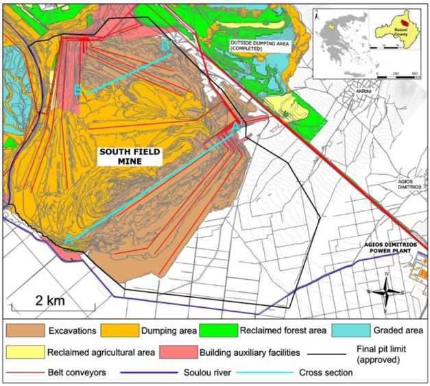
The South Field Mine (SFM) forms the southern boundary of the total Ptolemais mining area (Figure 1). It extends approximately 8 km towards the northwest and the southeast. Its SW–NE extension ranges between approximately 5 km in the northwest and 4 km in the southeast.

Approximately 30% of the overburden formations consist of hard and semi-hard material that cannot be excavated by BWE continuous mining system [29]. The hard formations in lignite mines consist of fine and coarse clastic sediments such as clays, marls, gravel, and conglomerates with embedded hard layers of sandstones, cemented conglomerates, and mudstones [30,31]. The average specific weight of the overburden is 19.62 kN/m³ (2 ton/m³), and the bulking factor ranges from 1.4 to 1.5. The average thickness of overburden material is 90 m.

The series of the overburden rocks of the SFM can be distinguished according to the rock coloration and way of formation into the following groups:

Red to brown clastic sediments: This group consists mainly of clays, conglomerates, and limestone gravels. The thickness of the whole formation is about 25 m, while the average thickness of hard material is approximately 10 m.

Gray to yellow clastic sediments: This group consists of clay, sandstones, sand, conglomerates, and siltstones. The average thickness of the whole formation is 25 m, while the average thickness of the hard material is 11 m.

Green-gray clay, sand, and silt sediments: The thickness of this formation varies from 25 m to 50 m. No hard material has been found in this formation.

The extent and the distribution of hard and semi-hard formations in the overburden strata are presented in the geological section of Figure 2.

Water outlets from the coarsely clastic sediments have been observed in the opencast mine. Furthermore, these layers, which principally consist of conglomerates, sandstone, and calcareous marl, locally incorporate consolidated intercalations, seriously impeding mining operations [30].

2.2. Dataset and Discretization

PPC created an extended borehole network throughout the SFM by drilling 777 exploratory boreholes (Figure 3).

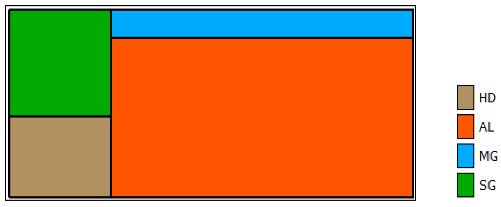
The borehole dataset contains information on 51,783 core samples. Sample lengths range from 0.01 to 213 m, with an average value of 2.5 m. and a standard deviation of 6.8 m. The large number of samples in each borehole and the diversity of sample lengths are due to the strong multi-seam character of the deposit and the variation of the quality characteristics between the seams [1]. For simplicity reasons, the geological descriptions of the samples were grouped into five lithotypes: hard rock formations (HD), clay (AL), marl (MG), sand with gravels (SG), and lignite (CO) (Figure 4). The (HD) formations consist of conglomerates, claystone, sandstone, and marly limestone; the (AL) of clay, soil, silt, and losses; the (MG) of marls and chalk; the (SG) of sand and gravels; the (CO) of coal (lignite). The aforementioned geological formations are interpreted in the photo of SFM presented in Figure 5. The spatial distribution of HD facies causes significant problems and delays since bucket wheel excavators cannot dig the entire face of the bench (see in the photo of Figure 5 the traces of bucket teeth stop in the lower marly limestone seam).

The overburden area can then be defined between the earth’s surface and the geological rooftop of the lignite orebody, as seen in Figure 6. This domain is divided into 58,609 horizontal parallelepiped blocks sizing 100 m × 100 m × 10 m each. For functionality reasons, the drills’ data were discretized in the 3D overburden grid, and a lithofacies value was assigned to each block crossed by a borehole. This operation was accomplished in two steps. First, the boreholes were cut into regular samples of 10 m, a size that corresponds to the depth of the basic grid cell. Then, after compositing, these regularized samples were migrated to the closest grid block so a single lithotype value would be assigned to the blocks crossed by a well. These blocks will, this way, become the conditioning data in the lithofacies simulation process.

2.3. Methods

Geological modeling is different from the usual geostatistical applications in mining, in the sense that it confronts the need to simulate categorical instead of numerical variables, such as the geological facies. The usual alternatives to treat this problem, when in covariance-based geostatistics, are to use the traditional Sequential Indicator Simulation (SIS) or the PGS, the second being most appealing and mathematically rigorous [32,33,34]. On the other hand, Multiple Point Geostatistics (MPG) is more appropriate to capture very complex and channelized facies [22] and is preferentially applied in under- or over-informed models and usually in groundwater or petroleum exploration [35].

The idea behind SIS is to simulate each category of the study variable in every location with an indicator, i.e., 0 or 1, thus having as many indicators as the categories. PGS, instead, can use only one artificial (hidden) continuous variable that is conveniently truncated to as many intervals as the real categories are.

More rigorously, in PGS, the idea is to represent and model the lithofacies using one or more hidden continuous Gaussian Random Functions (GRFs) at every point of the study area and then to convert them back to facies using a coding function:

Consider a vector of standardized (GRF) $\mathrm{Z}\left(\mathrm{x}\right)=\left({\mathrm{Z}}_1\left(\mathrm{x}\right),\cdots ,{\mathrm{Z}}_{\mathrm{q}}\left(\mathrm{x}\right)\right)$ where $\mathrm{x}\in {\mathrm{R}}^3$. Let $\left({\mathrm{D}}_1,\dots ,{\mathrm{D}}_{\mathrm{k}}\right)$ be a measurable partition of ${\mathrm{R}}^{\mathrm{q}}$ into $\mathrm{k}$ disjoint subdomains. A categorical random field $\mathrm{F}$ with $\mathrm{k}$ categories ${\mathrm{F}}_{\mathrm{i}}, \mathrm{i}=1,\cdots ,\mathrm{k}$ is then obtained by letting

$$\forall \mathrm{x}\in {\mathrm{R}}^3, \mathrm{F}\left(\mathrm{x}\right)=\mathrm{i}, \mathrm{if} \mathrm{and} \mathrm{only} \mathrm{if} \mathrm{Z}\left(\mathrm{x}\right)\in {\mathrm{D}}_{\mathrm{i}}$$

(1)

while the indicator random field for each facies ${\mathrm{F}}_{\mathrm{i}}$ is defined as:

$$\forall \mathrm{x}\in {\mathrm{R}}^3,{\mathrm{I}}_{{\mathrm{F}}_{\mathrm{i}}}\left(\mathrm{x}\right)=\{\begin{array}{c}1 \mathrm{if} I\left(\mathrm{x}\right)=i\hfill \\ 0 \mathrm{otherwise}\hfill \end{array}$$

(2)

The proper selection of the partition $\left({\mathrm{D}}_1,\dots ,{\mathrm{D}}_{\mathrm{k}}\right)$ is very important in the arrangement of categories, as we will show below, because it defines the permissible contacts and characterizes the spatial distribution of facies [34].

Then, one can approximate the proportion of a particular facies ${\mathrm{F}}_{\mathrm{i}}$ at point $\mathrm{x}$ by the probability of having these facies ${\mathrm{F}}_{\mathrm{i}}$ at that point $\mathrm{x}$:

$${\mathrm{P}}_{{\mathrm{F}}_{\mathrm{i}}}\left(\mathrm{x}\right)=\mathrm{P}\left\{\left({\mathrm{Z}}_1\left(\mathrm{x}\right),\cdots ,{\mathrm{Z}}_{\mathrm{q}}\left(\mathrm{x}\right)\right)\in {\mathrm{D}}_{\mathrm{i}}\right\}=\underset{{\mathrm{D}}_{\mathrm{i}}}{{\displaystyle \int }}{\mathrm{g}}_{\mathsf{\Sigma }}\left({\mathrm{Z}}_1\left(\mathrm{x}\right),\cdots ,{\mathrm{Z}}_{\mathrm{q}}\left(\mathrm{x}\right)\right){ \mathrm{dZ}}_1\cdots {\mathrm{dZ}}_{\mathrm{q}}$$

(3)

where ${\mathrm{g}}_{\Sigma }\left({\mathrm{Z}}_1\left(\mathrm{x}\right),\cdots ,{\mathrm{Z}}_{\mathrm{q}}\left(\mathrm{x}\right)\right)$ is the q-variate Gaussian density of $\mathrm{Z}\left(\mathrm{x}\right)$ and $\Sigma$ its covariance matrix.

In order to compute ${\mathrm{P}}_{{\mathrm{F}}_{\mathrm{i}}}$ it is enough to know the ${\mathrm{D}}_{\mathrm{i}}$’s of the chosen partition, but the inverse is, in general, not true because there can be many solutions to the problem. This means that one has a degree of freedom here to decide the spatial arrangement of ${\mathrm{D}}_{\mathrm{i}}$’s. and it is here where the empirical geological knowledge can conveniently enter the scene under the “geological rule”. To ease the solution, the partitioning of the Gaussian space is affected into cuboids defined by their projections on the Gaussian axes. The endpoints of the projections on each axis are then considered thresholds. In practical applications, the proportions of facies are known experimentally from core data by calculating the Vertical Proportion Curves (VPCs), so the $\mathrm{k}\times 2^{\mathrm{q}}$ thresholds should be determined together with the definition of the geological rule. This can be achieved by numerically inverting Equation (3).

After the definition of the geological rule that describes the sets associated with each category, the second integrant to be determined for the complete specification of the plurigaussian model is the multivariate variogram functions of the underlying GRFs. These variograms represent the structural characteristics of the physical phenomenon, such as spatial continuity and anisotropies; however, the inference of this variogram model is one of the major difficulties associated with the use of the plurigaussian model [8]. This is because, while the available information restricts the experimental indicator variograms and cross variograms of the facies, the required variogram models are ones of the underlying GRFs, which are hidden by the truncation procedure; therefore, these models, which represent the spatial continuity of facies, were usually determined by a trial and error procedure, using, for example, the program VMODEL [36]. In this work, we use an algorithm based on the Pairwise Likelihood (PL) maximization principle to directly estimate the variograms of the underlying GRFs [37].

After the definition of the model variogram of $\mathrm{Z}\left(\mathrm{x}\right)$, the Gibbs sampler is used to generate Gaussian values at the sample points that have the appropriate covariance and belong to the right intervals. Then, a conditional simulation is used to produce several realizations conditional to the Gaussian values at the above points. At the end of the process, the Gaussian values of the realizations are converted to facies using the truncation rule.

3. Results and Discussion

3.1. Structural Analysis and Spatial Modeling

First, care should be taken so that the simulation results are consistent with the deposition process, meaning that calculations have to be performed inside layers conforming to the deposition beds in order to attend the stratifying order. An approach to secure these geological restrictions is to work in a flattened domain while the flattening process confronts the sedimentogenesis model. In the present work, the Isatis.neo™ algorithm was used to unfold the working grid parallel to the top surface (Figure 7).

Next, the proportions of each lithotype have to be estimated in each block of the flattened grid. These proportions are important ingredients of the modeling process because, as mentioned in the previous paragraph, they approximate the probability of having certain phases at a specified block, and so they constitute the soft constraints of the plurigaussian model. The proportions are estimated from the borehole data in three dimensions (3D) using an interpolation approach based on Stochastic Partial Differential Equations (Figure 7). Finally, the lithological rule, which embodies the empirical geological knowledge concerning lithofacies contacts, complementary to the proportions, allows the calculation of the phase’s probabilities, as shown in Figure 8.

After the estimation of the proportions and the lithological rule, the last ingredient for the complete determination of the plurigaussian model is the variograms of the two underlying GRFs. In the present study, these variograms are calculated directly from Gaussian values assigned to the lithotype samples, as previously mentioned [37]. The variogram of the first GRF is a spherical scheme with a horizontal range of 300 m, and an anisotropic vertical range of 30m. The variogram of the second GRF is an exponential model with sill = 1, a horizontal range of 400 m, and an anisotropic vertical range of 200 m (Figure 9).

The main part of the plurigaussian simulation is performed in four steps: First, a Gibbs sampler was used to conditionally simulate the two GRFs on the data points by assessing the right Gaussian values to the experimental lithofacies. Second, the two GRFs were unconditionally simulated at each block of the flattened working grid. Then, the realizations of the second simulation were conditioned on the results of the first step. Finally, the Gaussian outputs of the last simulations were inverted to lithofacies by using the thresholds calculated by the combination of the lithotypes proportions and the lithological rule.

The last thing to perform is to copy the simulation results from the unfolded grid to the original domain by using the inverse geometrical transformation. An overview of the resulting plurigaussian model realization is shown in Figure 10.

3.2. Validation of the Results

Unlike estimation, where the best map is sought under a certain optimality criterion (for kriging, it is the minimization of the mean square error), in geostatistical simulations, the main concern is to provide maps that reproduce the spatial variability of the study variable. As a result, different realizations are produced, and there is not a single best realization, since they are all considered equally likely to occur. This distribution of outcomes is interpreted as the uncertainty of the variable and thus allows us to explore the risk associated with the produced model of reality. As previously stated, in our case, this risk is connected to the average cost of discontinuously removing the hard rock volumes of overburden formations.

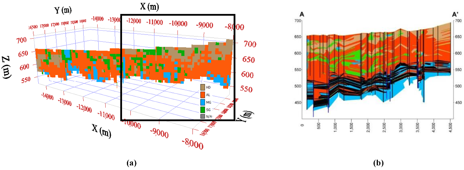
Validation of simulation results cannot rely on a point-wise comparison but rather on examining the average match of estimated images to reality. In our case, we examine the similarity of our model to reality in two available experimental cross sections, AA’ and BB’, the traces of which are presented in Figure 1 and Figure 2.

Figure 11and Figure 12 show that the shapes and relative volumes of the overburden formations are, in general, similar to the realistic geological cross-sections.

A more straightforward way, though, to validate the model results is to compare the volume of the assessed hard rock formations to the actual one. In this framework, PPC has available accounting volumetric results in quite a large area on the northern part of the orebody, as shown in Figure 13 and Figure 14. In order to calculate these actual results in the ArcGIS environment, the top and bottom surface elevation models were elaborated with value ranges from 670 m. a.s.l. to 740 m. a.s.l. The top surface is considered the natural topographic relief, whereas the bottom surface is considered the hard formations excavated surface up to a specific terrace. By using the “surface difference” tool from the ArcGIS 3D Analyst Toolbox, the volume calculation was affected inside the defined volume calculation polygon. The total area amounts to 8,500,000 m³, while the company’s reported hard rock volume in this area amounts to 1,700,000 m³.

In order to check these results with the model output, the top and bottom surfaces were entered into the grid to define the calculation domain. Finally, a number of 84 grid blocks were found inside this part of the model. In a total of 100 simulations, an average percentage of 18 blocks was characterized as HD, which means that a total of 1,800,000 m³ are expected to be met here. This is quite in accordance with the company’s reported results, which, as previously mentioned, amount to 1,700,000 m³ in the examined area.

Considering the improvement of the results obtained by the suggested method, it could be noted that this approach can offer a more accurate prediction regarding the spatial distribution of various rock lithofacies in broader mining sectors of coal or other surface mines. In addition, complicated structures of the overburden material can be successfully modeled and simulated more efficiently than indicator kriging or other similar categorical simulation methods stated in the introduction. Furthermore, the analysis can be extended to other types of rocks, such as water-permeable rocks.

4. Conclusions and Future Research

Plurigaussian simulations can be successfully applied to the overburden lithofacies of the South Field Mine by using the plethora of accessible core data with geological descriptions.

The available field data, such as cross-sections drawn on mine slopes and actual production data from specific areas of non-continuous mining equipment operations, can be used to calibrate the model parameters, such as the unfolding of the working domain and the regularization of core samples.

Validation of model results showed that the estimated thickness and quantities of the hard rock formations in broader mining sectors agree with the available PPC accounting volumetric data.

Thus, model predictions can be successfully used for the optimization and scheduling of the mining process by minimization of the delays from changing the machinery arrangements when hard rock formations are encountered. This approach can be incorporated into the mine planning and design procedures, emphasizing the mining cost minimization considering a better mine production scheduling. In this context, the improved spatial interpolation of hard rock formations could support better planning and scheduling of non-continuous mining equipment in specific mining sectors and also the strategic planning of continuous surface mining equipment (e.g., bucket wheel excavators). Significantly, if the developed methodology could be incorporated from the first stages of the strategic mining plan, it could help to achieve the mining sustainability goals (e.g., environmental by minimizing the impacts of non-continuous mining, or economic ones by minimizing the mine production costs, also considering the delays from changing the mining machinery arrangements).

Possible limitations of the applied method include the need for accurate interpretation of borehole samples and a suitable definition of the lithological rule based on geological experience.

Future research could focus on examining multiple-point statistics, an alternative method for lithofacies modeling and prediction of hard rock spatial distribution.