Article

Magnetotelluric Noise Attenuation Using a Deep Residual Shrinkage Network

1
School of Geoscience and Info-Physics, Central South University, Changsha 410083, China
2
Shenzhen Research Institute of Central South University, Shenzhen 518057, China
3
Key Laboratory of Metallogenic Prediction of Nonferrous Metals and Geological Environment Monitoring (Ministry of Education), School of Geosciences and Info-Physics, Central South University, Changsha 410083, China
4
School of Geophysics and Measurement-Control Technology, East China University of Technology, Nanchang 330013, China
*
Authors to whom correspondence should be addressed.
Minerals 2022, 12(9), 1086; https://doi.org/10.3390/min12091086
Submission received: 22 March 2022 / Revised: 19 August 2022 / Accepted: 20 August 2022 / Published: 27 August 2022
(This article belongs to the Special Issue Electromagnetic Exploration: Theory, Methods and Applications)

Abstract

:
Magnetotelluric (MT) surveying is an essential geophysical method for mapping subsurface electrical conductivity structures. The MT signal is susceptible to cultural noise, and the intensity of noise is growing with urbanization. Cultural noise is increasingly difficult to be removed by conventional data processing methods. We propose a novel time-series editing method based on the deep residual shrinkage network (DRSN) to address this issue. Firstly, the MT data are divided into small segments to form a dataset system. Secondly, we use the dataset system to train the denoising model. Finally, the trained model is used for MT data denoising. The experiments using synthetic data and actual field data collected in Qinghai and Luzong, China, show that the DRSN can effectively remove the cultural noise and has better adaptability and efficiency than traditional MT signal processing methods.

1. Introduction

The magnetotelluric method has been widely used in geophysical exploration to investigate Earth’s deep electrical structure [1,2,3,4]. It is based on the relationship between the electric fields and the magnetic fields measured on the Earth’s surface, which can be expressed as follows:
E = Z H
where E , H and Z denote the electric field, the magnetic field, and the impedance tensor, respectively. Then, the apparent resistivity ρ and phase ϕ were calculated as follows:
{ ρ = 1 ω μ | Z | 2 ϕ = arctan ( Im ( Z ) Re ( Z ) )
where ω is the angular frequency, μ is the magnetic permeability of free space, and Z is the impedance tensor; the real part of Z is denoted as Re(Z), and the imaginary part is marked as Im(Z).
The sources of the MT method are lightning activities at high frequencies and the current magnetospheric current flows excited by solar wind at low frequencies [5]. The MT signal is non-stationary and broadband. It can be easily affected by cultural noises, from power lines, railway lines, road vibration, and vehicles [6]. Noisy MT data have low reliability and interpretability for deep structure detection. Improving the quality of MT data can make the subsequent inversion more reliable [7,8].
Classical denoising methods are the remote reference (RR) method, the robust method, and the time domain signal–noise separation method. RR uses the correlation between the magnetic fields of the measuring station and those of the reference station to improve the quality of the apparent resistivity and phase curves [9]. It can separate signal and noise when signals are correlated and noises are uncorrelated [10]. However, in the case of continuous and cultural solid noises, choosing remote reference stations becomes very difficult [11]. The robust method does not depend on remote reference stations. It is a power spectrum selection method [12,13]. The robust method may lead to erroneous results if the noise is continuous and intense during the whole observation process [14,15,16]. The signal–noise separation methods in the time domain can effectively remove intense cultural noises [17,18,19,20,21,22]. However, these methods have their limitations [22]. For example, these methods are more or less prone to damage to low-frequency effective signals and require manual intervention [23,24].
Deep learning algorithms have recently been applied to process geo-electromagnetic datasets [25]. For instance, the authors of [26] used the self-organizing feature map (SOM) neural network combined with the data segment selection method to remove the cultural noise in MT data. The authors of [27] employed the wavelet neural network to eliminate the noise generated by high-frequency motion in helicopter airborne transient electromagnetics. The authors of [28] used the long short-term memory (LSTM) neural network to remove power frequency noise.
After flowing through some layers of the convolutional neural network (ConvNet), the gradients of the error function become inaccurate. Residual Network (ResNet), a ConvNet variant, uses identity shortcuts to optimize the parameters [29]. It has been applied in signal denoising [30] but has poor feature learning ability for highly noisy MT data. New methods were needed for removing magnetotelluric noise under a robust noise environment.
In 2019, the deep residual shrinkage network (DRSN) model was proposed for improving the feature learning ability of low signal-to-noise ratio (SNR) signals [31]. It has been successfully used in signal recognition [31,32,33]. The DRSN model excavates the substrate features of the data and can extract hidden features without using prior knowledge. So, it provides more accurate and effective denoising results.
This study uses the DRSN for MT noise suppression. To improve the feature extraction ability, we add the Squeeze-and-Excitation Network (SENet), a deep learning method based on attention mechanism and a soft threshold function, to DRSN.
This method has three advantages. Firstly, it does not require professional signal processing knowledge and can adaptively select the noise threshold for MT denoising. Secondly, it can directly separate the signal and noise of MT data collected in various regions. Thirdly, using one-dimensional data can extract essential features from time series signals and avoid dimension transformation.
The rest of this study is arranged as follows. Section 2 introduces the DRSN model. Section 3 validates the DRSN model using synthetic and real MT datasets. In Section 4, the advantages and limitations of this method are discussed. Section 5 presents conclusions.

2. Methods

2.1. The DRSN Method

The DRSN is a deep learning method that can extract hidden features without prior knowledge, providing more accurate denoising performance. The residual building unit of the DRSN (RSBU) structure is shown in Figure 1.
DRSN has two types:
(1)
DRSN-CS has the block of “residual shrinkage building unit with channel-shared thresholds (RSBU-CS)”.
(2)
DRSN-CW has the block of “residual shrinkage building unit with channel-wise thresholds (RSBU-CW)”.
DRSN-CW is more effective than DRSN-CS in removing the noise because different channels of the feature map usually contain different amounts of noise-related information [30]. We adopt DRSN-CW and call it DRSN hereafter.
The structure of the proposed network is shown in Figure 2. RSBU (4,3,/2) means an RSBU has 4 convolutional kernels with a width of 3, and “/2” represents a step length of 2. In the RSBUs, three RSBUs were followed when the previous DRSN’s step length was 2, and there were 12 RSBUs. The residual module, BN layer, and threshold subnetwork were used to achieve regular training. The learning rate decreased exponentially from 0.001 to 0.0001, and the number of training cycles was 200. However, the training process will stop if the loss has no change within ten cycles.

2.2. Principle of MT Denoising by DRSN

2.2.1. Soft Threshold Function

The most representative time-series editing method is the soft threshold method. The soft threshold function is as follows:
y = { ( | x | τ ) sign ( x ) , | x | τ 0 , | x | < τ ,
where x , y are the input feature and the output feature, respectively, and τ is the threshold with a positive value.
The partial derivative of the soft thresholding function is as follows:
Δ y Δ x = { 1 x > τ 0 τ x τ 1 x < τ ,
The partial derivative of the soft thresholding function is either 1 or 0; thus, we can perform the signal–noise separation.

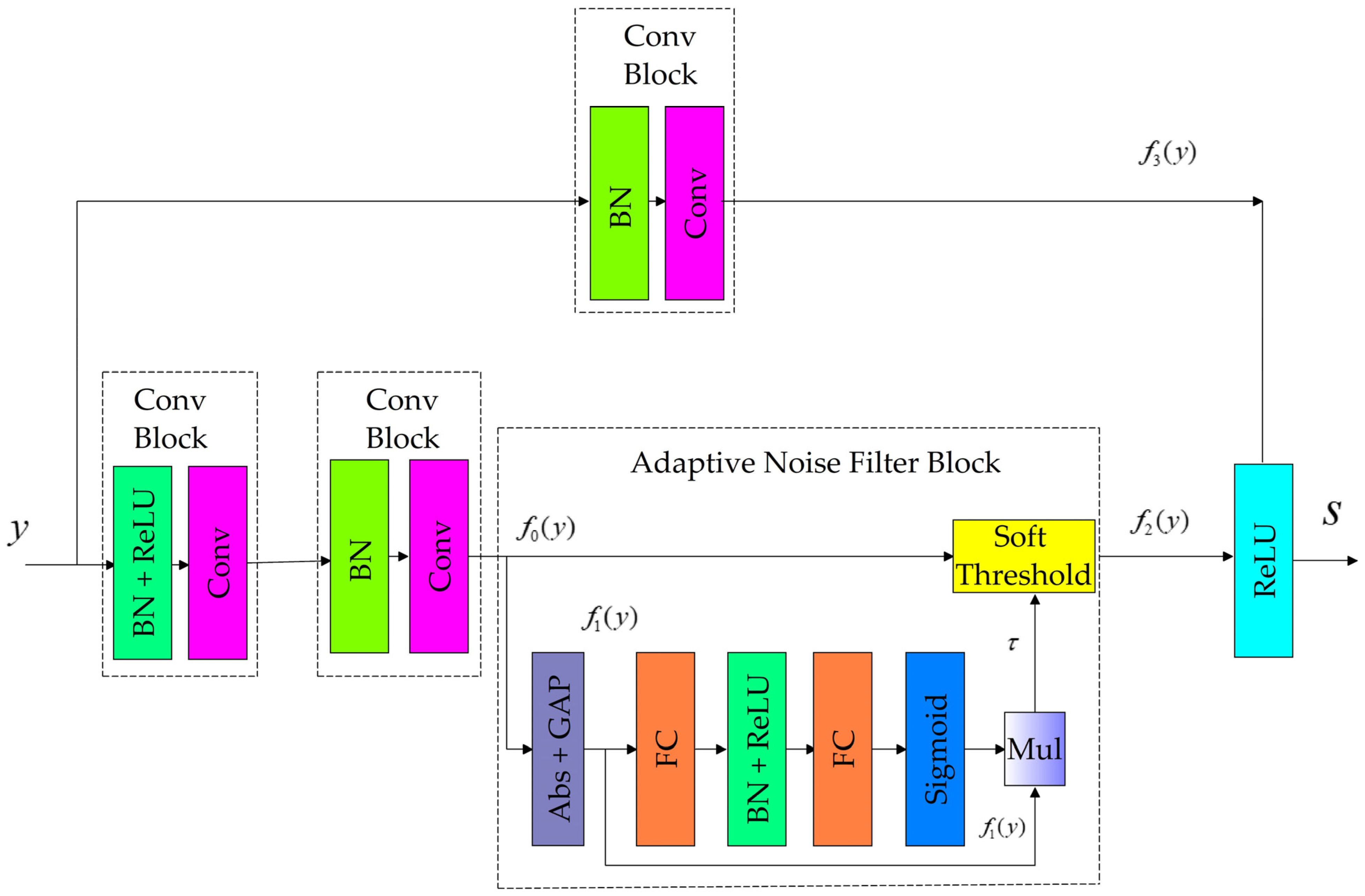
2.2.2. Adaptive Noise Filter Block

The noise features are first extracted through the ResNet Block, and then a one-dimensional vector with an absolute operation ( A b s ) and a G A P layer is used to reduce the feature map size.
f 1 ( y ) = G A P ( A b s ( f 0 ( y ) ) ) ,   f 1 ( y ) R C × 1 × 1
Moreover, the number of neurons in the F C layer is the same as the number of channels from the input feature map. Then enters the two full connection layers a scale factor is obtained,
α = F C ( R e L U ( B N ( F C ( f 1 ( y ) ) ) ) ) ,   α R C × 1 × 1
The scale factor is normalized to the range of (0, 1) by a sigmoid function. The threshold value of filtered noise features was obtained by multiplying the normalized result f 1 ( y ) .
τ = S i g m o i d ( α ) × f 1 ( y )
After the soft threshold processing, the noise-related features are removed.
f 2 ( y ) = s t f ( f 0 ( y ) , τ )
where s t f ( ) represents the soft threshold function for filtering features generated by the noises.
To enhance the nonlinearity and the fitting capability, we apply the R e L U functions defined as follows:
f R ( a ) = m a x ( a , 0 )
where a represents the variable output from the neural network cell in the upper layers.
Finally, we have the relationship between input y and output s as follows:
s = R e L U ( f 2 ( y ) + f 3 ( y ) )
where f 2 ( y ) denotes the function of the below layer in Figure 1, f 3 ( y ) denotes the function of the above layer in Figure 1, and R e L U is the rectified linear unit. Thus, f 3 ( y ) only changes the channels (e.g., the stride in this block is set to 2, which results in different sizes between the input and output of this block) and does not influence the value of y . That is to say, s can still acquire the information of y from f 3 ( y ) .
The hardware resources of the computer used for the processing in this study are as follows:
-
CPU: Intel i7-9700K, 3.00 GHz, 8×;
-
GPU: Nvidia GeForce RTX 2060 SUPER, 8 GB;
-
RAM: 16 GB.

2.3. Datasets

We obtained the dataset by adding simulation noise to measure high-quality data. Our team collected the high-quality MT data in 2012 in the Qaidam Basin of Qinghai Province, China. There was almost no interference. The MTU-5A collected the data from Phoenix Geophysics Ltd. The MT data can be used as noise-free signals. The software for these field data acquisitions and apparent resistivity and phase computations is SSMT-2000 (Version 0.6.0.70, Phoenix Geophysics Ltd., Toronto, Ontario, Canada).
We cut the actual MT data using windows and corrupted them using the artificial noise, such as the harmonic, square, triangle, impulse, and step noises, and the noise-free data were the label for forming datasets (Figure 3, Figure 4, Figure 5, Figure 6 and Figure 7). We had 22,000 datasets: 20,000 datasets for training and 2000 for verification. The training set performed denoising training on the DRSN so that the DRSN learned the mapping relationship between the noise-free data and the corresponding noise. Once the DRSN completed training, we fed the MT data sections into this DRSN. The outputs of the DRSN were the denoising MT signals. We used data from multiple places to produce the training set.

2.4. Training the DRSN for Denoising

Figure 8 shows the flow chart of the denoising process using the DRSN. Firstly, we use the time window to scan and segment the 1D MT data. We take the 1D rather than the 2D data to reduce the calculation time and resources. Secondly, the DRSN is used for noise suppression to obtain noise-free MT signals. The training set performs denoising training on the DRSN so that the DRSN learns the mapping relationship between the noise-free data and the corresponding noise. Once the DRSN completes training, those data sections are fed into this DRSN. The outputs of the DRSN for suppression are the denoising MT data.
We train the DRSN in two steps:
  • Hyperparameter setup
The hyperparameters were set as follows: mini-batch size 100, dropout 0.5 in full connection, initial learning rate 0.0001 that decreases 95% every five epochs.
2.
Optimize hyperparameters through training
Our DRSN has a nine-layer structure for denoising the magnetotelluric data. We use common training strategies to achieve faster convergence, such as the Adam optimization algorithm [34] and mini-batch training mode. The L2 norm can be used to optimize the parameters of neural network.
In training, the samples with noise are input into DRSN, and the samples without interference are the output. Forward propagation was used to obtain network parameters, and backpropagation was used to adjust network parameters.
The residual module, BN layer, and threshold subnetwork were used to achieve regular training. The learning rate decreased exponentially from 0.001 to 0.0001, and the number of training cycles was 200. However, the training process will stop if the loss has no change within ten cycles.

3. Experiments

3.1. Simulation Data Experiments

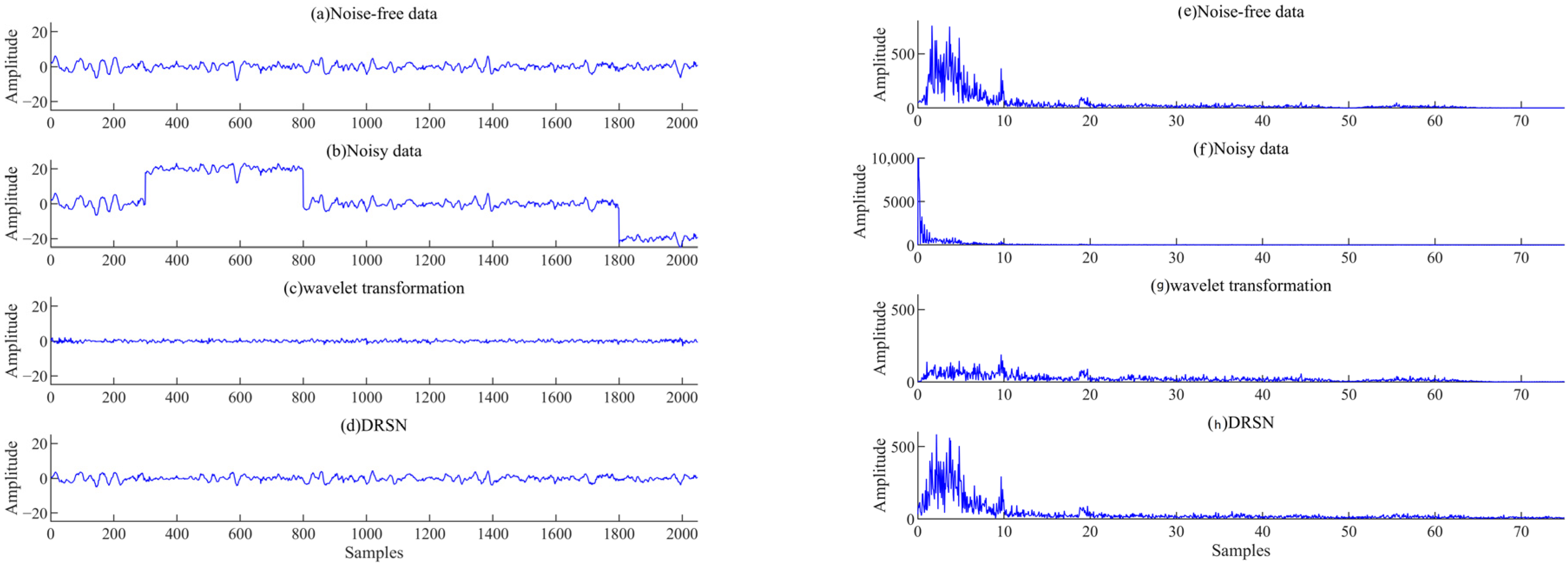
3.1.1. Comparison with Wavelet Transformation and VMD

We validated the proposed method using a simulated dataset with step-wave noise, which is typical for MT data.
First, we chose the noise-free signal from actual MT data, to which we added step-wave noise using a simulated dataset with step-wave noise. Then we used the trained DRSN model to separate signal and noise. We also denoised the data by using the wavelet transformation method and VMD, and the results are compared in Figure 9.
After signal processing, the noise was suppressed (Figure 9). As Figure 9f–h shows, compared with the noise-free spectrum, the results obtained by the wavelet transformation and VMD lose some low-frequency effective signals. However, our method yields no visible distortion.
We compare the normalized mutual correlations (NCCs) of the denoising results obtained by different methods in Table 1. NCC is often called similarity degree. When the NCC value is 1, two signals are the same; when the NCC value is 0, two signals are orthogonal; when the NCC value is −1, two signals have the same absolute value but opposite signs. Therefore, the closer the NCC value to 1, the better the separation effect [35]. In addition, we use the signal-to-noise ratio (SNR) to evaluate the denoising results.
NCC = n = 1 N y ( n ) r ( n ) ( n = 1 N y 2 ( n ) ) ( n = 1 N r 2 ( n ) )
SNR = 10 log 10 ( y ( n ) 2 y ( n ) r ( n ) 2 )
where y ( n ) is the noise-free signal, r ( n ) is the denoised signal, and N is the length of the signal.
As Table 1 shows, the result obtained by our method has the highest NCC and SNR, so our approach has the best denoising effect.
After denoising the wavelet transformation, VMD and DRSN find the noise is attenuated (Figure 8).
However, compared with the original spectrum, it is clear that the results obtained by DRSN, the noise-free data section, can be protected well simultaneously.

3.1.2. Comparison with Other Deep Learning Models

To further verify the effectiveness of the DRSN, we compare it with the ConvNet and the ResNet. Several field MT time series with harmonic, square, triangle, impulse, and step noises were used for training the models. We introduced all the models with a one-time window (size 1 × 32 ). Their performances are evaluated by the training loss and computational time (Figure 10). The parameters of these models are shown in Table 2.
The first column of Table 1 shows the number of blocks in different layers.
The second column shows the output sizes of the feature maps in different layers, which are in the 3-D form of c h a n n e l s × w i d t h ×   height . For example, 1 × 256 × 1 means that the channel is 1, the width is 256, and the height is 1 (because it is 1D signal).
In the third column, CBU (4,3,/2) means a CBU has four convolutional kernels with a width of 3. “/2” represents CBU can reduce the width of the feature map by moving the convolutional kernels with a stride of 2. Other items have the same meaning.
Figure 10 presents the loss of training and validation datasets of the three deep learning methods for MT noise suppression, which both descend gradually as the number of epochs ascends. Both loss curves are stable, proving the generalization of the three deep learning methods. Because the DRSN reaches the stationary stage of both loss curves earlier than the ResNet, the DRSN has a better generalization capability than the ResNet. The training and test errors of the DRSN are much more minor than those of ConvNet and ResNet. This confirms that using the identity shortcuts, the attention mechanism, and the soft threshold function can improve parameter optimization.
We also investigate the influence of window size on the accuracy of the proposed method. We adopt four different window sizes, 1 × 32 , 1 × 64 , 1 × 128 , and 1 × 256 , for the validation datasets (Table 3).
Table 3 shows that the window size influences denoising accuracy and training time. As the window size grows, the DRSN’s training becomes more time-consuming. In addition, the losses are nearly equivalent when the window sizes are 1 × 64 , 1 × 128 , and 1 × 256 and are smaller than the loss of 1 × 32 . Hence, we choose the window size of 1 × 128 to balance the loss and running time of the DRSN.
We also compare the DRSN method with other methods regarding training time and loss (Table 4). The window sizes were set as 1 × 32 . As shown in Table 3, the DRSN has the minimum training loss and the longest training time.
We used data by adding simulation noise to measure high-quality data. First, we chose the noise-free signal from Qinghai in 2012, to which we added simulation noise. Then, we used the trained ConvNet, ResNet, and DRSN to separate signal and noise (Figure 11).
We compare the time series of the data denoised by different methods (Figure 11) and find the noise was attenuated, and the noise-free data section can be protected well.
As Table 5 shows, the result obtained by our method has the highest NCC and SNR, so our method has the best denoising effect.
We used data by adding simulation noise to measure high-quality data. First, we chose the noise-free signal from Luzong in 2010, to which we added simulation noise. Then we used the trained ConvNet, ResNet, and DRSN to separate signal and noise (Figure 11).
We compare the time series of the data denoised by different methods (Figure 12) and find the noise was attenuated, and the noise-free data section can be protected well.
As Table 6 shows, the result obtained by our method has the highest NCC and SNR, so our method has the best denoising effect.

3.2. Actual Data Experiments

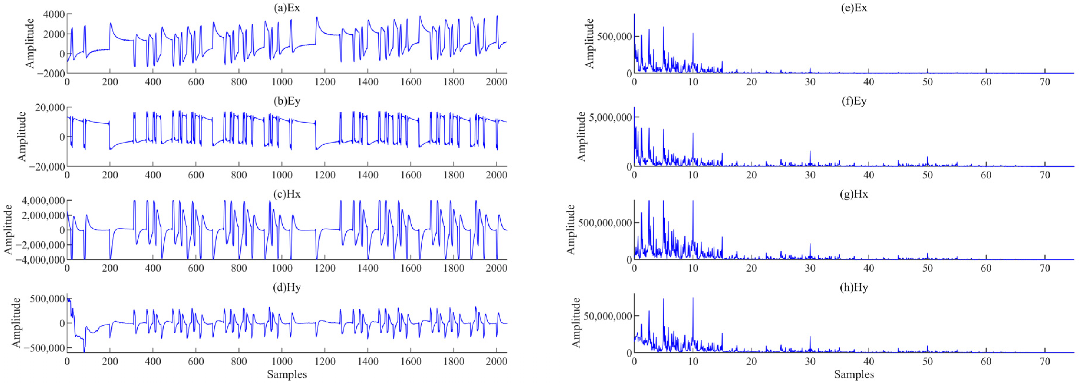
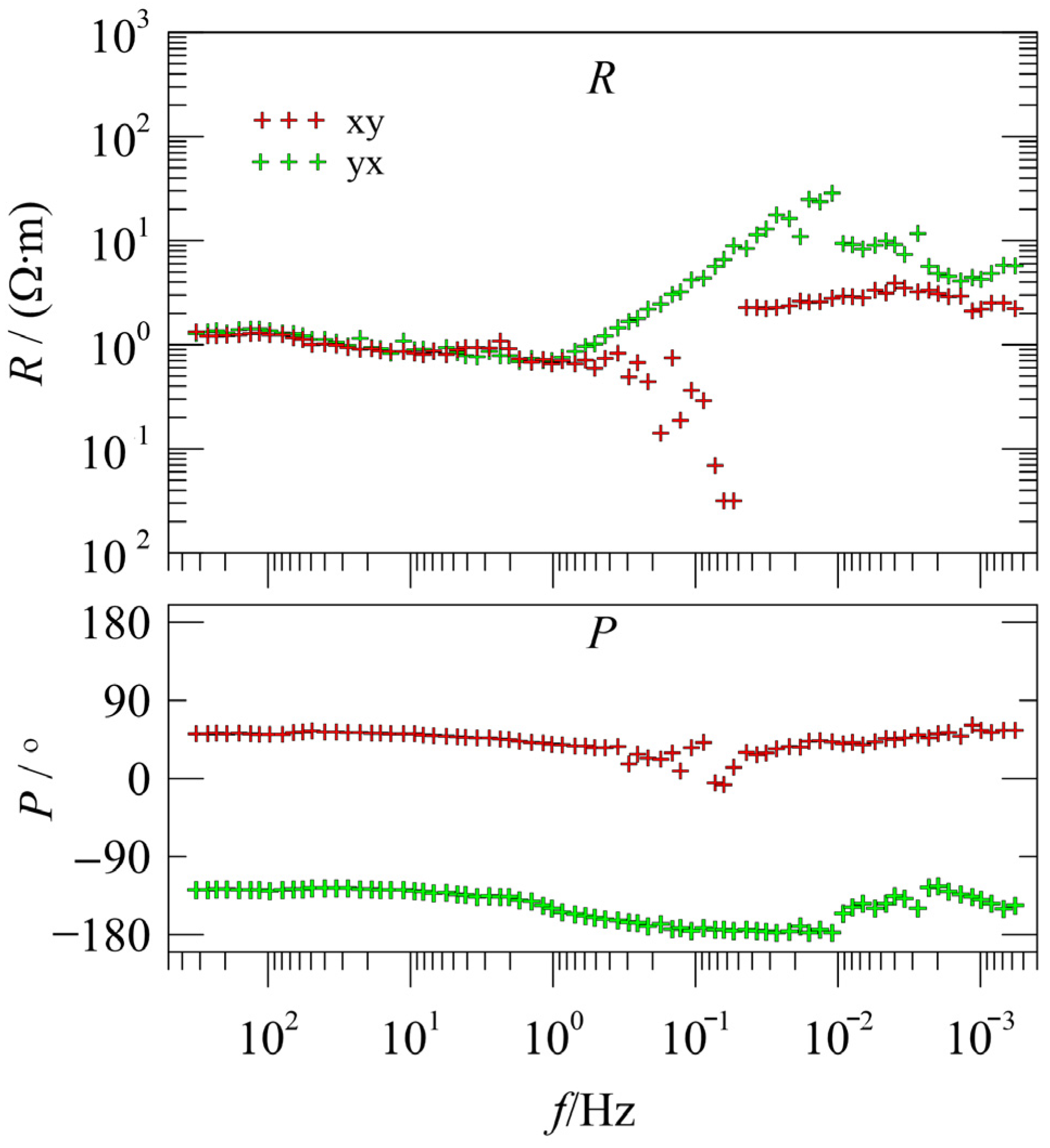
3.2.1. Experimental Data in Qaidam Basin

We validated our method using the MT data collected in 2012 in the Qaidam Basin of Qinghai Province, China. There is almost no interference. The MTU-5A collected the data from Phoenix Geophysics Ltd. (Toronto, ON, Canada) and the controlled-source electromagnetic method (CSEM) transmitter from Central South University, China.
The sampling frequency was 15 Hz and the collection time was about 19 h, divided into two phases; the first was 1.5 h and the second was 17.5 h. In the first phase, a pseudo-random signal with the current of 80 A was injected into the ground 2 km from the measuring point by the wide field electromagnetic method (CSEM) so that our team collected the MT data under the interference of CSEM transmission. In the following 17.5 h, the transmitter stopped working, so there was almost no interference.
The apparent resistivity, phase, and polarization direction were used to evaluate the MT denoising performance [36].
Figure 13 shows the fragment of the noisy signal in the time domain collected in the first 1.5 h. The CSEM severely pollutes the data.
As shown in Figure 13, the time domain waveforms present periodicity and regularity, and the MT waveforms were almost submerged. As shown in Figure 14, the apparent resistivity and phase curves in the whole period are discontinuous and not smooth. The apparent resistivity and phase curves jump sharply between 0.3 Hz and 0.05 Hz in the xy direction. In the yx direction, the pronounced resistivity curve rises 45° between 0.5 Hz and 0.01 Hz and drops sharply when the frequency is lower than 0.01 Hz. The phase is mainly close to −180° between 0.5 Hz and 0.01 Hz. In summary, the MT data have apparent near-source interference in the whole period [37].
Figure 13 shows that the waveform and spectrum in the time domain of each original noise-containing signal are almost the same as those of each separate noise corresponding to Figure 15.
Figure 16 shows the signal denoised by our method. Before denoising, the signals in the time domain present periodicity and regularity, and the MT signal is almost submerged. After denoising, the signals present randomness and irregularity, which are the features of a natural MT signal. In addition, the signal amplitude is small.
We compare the denoising performance of the proposed method and the robust method in Figure 17. After processing our way, the apparent resistivity and phase curves have good continuity and smoothness across all frequency bands. Between 0.5 Hz and 0.01 Hz, the pronounced resistivity curve of the robust method has a 45° rising trend in the yx direction, but that of DRSN only shows a slight upward trend.
We compare the two results in Figure 17. The apparent resistivity and phase curves after robust processing are not consistent with those of the undisturbed segment. Still, the results of our method coincide with the steady part, indicating that our approach is better than the robust method in processing the cultural noise.
As shown in Figure 18, the noise leads to polarization direction converging in some angles, such as the range 0° in Figure 18a,b, indicating that the data are subject to extreme interference. Figure 18c,d show that the noise-free data’s polarization directions become random in electric and magnetic fields. After denoising, their polarization directions become overall random in electric and magnetic fields (Figure 18e,f). Because the undisturbed magnetotelluric signal originates from the natural area, its polarization direction was randomly distributed due to the characteristics of the field source. However, after noise interference, the strength of the artificial source is greater than that of the natural field, making the polarization direction show the characteristics of the artificial field source, which is relatively concentrated and regular. These results demonstrate that our approach can remove MT noise well regardless of the noise level.

3.2.2. Experimental Data in Luzong

In 2010, we performed a magnetotelluric experiment in the Luzong mining area, Anhui Province, China, using V5-2000 from Phoenix Geophysics Ltd. Due to the developed economy, there is much cultural noise, so the MT signals have many abnormal time series. However, the noise is relevant and persistent, making it challenging to eliminate effectively by traditional methods.
As shown in Figure 19, there are many outliers in the curves of the raw data. When the frequency is below 40 Hz, the apparent resistivity changes linearly with the frequency, showing a 45° rise, and the phase approaches 0 or ±180°. The noise around the observation station contaminates these data, so the original curves cannot accurately reflect the electrical structure underground.
Figure 20 shows the apparent resistivity, and phase curves varied smoothly with frequency after DRSN treatment. The results obtained by our method are consistent with those obtained by the RR method, except for the data in the low-frequency band. It shows that DRSN can be effective in MT denoising.

4. Discussion

This study applied the deep residual shrinkage network for MT signal–noise separation. Testing shows that in noise mitigation, the DRSN outperforms traditional noise removal methods and deep learning methods such as ConvNet and ResNet. First, it directly uses the noisy raw data to train the model. Furthermore, the algorithm, benefiting from the end-to-end DRSN structure, can extract useful features from noisy data. Finally, DRSN has a better noise removal effect, shorter training times, and fewer overfitting risks.
It has limitations. For instance, it requires a longer training time than other deep learning algorithms.

5. Conclusions

Using the MT method to investigate underground structures requires high-quality time series, which are difficult to extract from noisy MT data. To address this issue, we propose a novel signal–noise separation method based on the deep residual shrinkage network. The method can learn features and separate signal and noise. The results are improved obviously in the time domain, spectrum, apparent resistivity, phase curve, and polarization direction. In addition, the method was based on a relatively simple deep learning network, so no professional signal processing knowledge is needed, resulting in a simple operation. The DRSN method is effective and intelligent, effectively adjusting the sample distribution and improving the data quality. Although its training time is extended, the denoising process only takes 1–3 s, making it much faster than other MT denoising algorithms. In addition, the DRSN method can remove unknown electric noise, correct the distortion of resistivity and phases, and randomize the distribution of electric and magnetic fields.

Author Contributions

Conceptualization, G.Z.; data curation, G.Z.; formal analysis, G.Z., L.Z. and G.L.; funding acquisition, Z.R., X.X., J.T., G.L. and G.Z.; investigation, G.Z., L.Z. and G.L.; methodology, G.Z. and L.Z.; project administration, G.Z.; resources, Z.R., X.X. and J.T.; software, G.Z.; writing—original draft, G.Z.; writing—review and editing, Z.R., X.X., J.T., G.Z., L.Z. and G.L. All authors have read and agreed to the published version of the manuscript.

Funding

This study was supported by the National Natural Science Foundation of China (41830107, 41922027, 41904076, 4214200052); the Shenzhen Science and Technology Program (JCYJ20210324125601005); the National Key R&D Program of China (2018YFC0603202); the Open Fund from Key Laboratory of Metallogenic Prediction of Nonferrous Metals and Geological Environment Monitoring, Ministry of Education (2021YSJS02); the Natural Science Foundation of Jiangxi Province (20192BAB212009; 20202BAB211011); the Fundamental Research Funds for the Central Universities of Central South University (2019zzts297); and Central South University Innovation-Driven Project (2020CX0012).

Data Availability Statement

The data discussed in this paper will be shared at reasonable request to the corresponding author.

Acknowledgments

We would also like to express our gratitude to Meixiang Huang for her helpful work in the formal analysis, investigation, methodology, and writing—review and editing. This work was carried out in part using hardware and/or software provided by the High Performance Computing Center of Central South University.

Conflicts of Interest

The authors declare no conflict of interest.

References

  1. Tikhonov, A. On determining electrical characteristics of the deep layers of the Earth’s crust. Dokl. Akad. Nauk. USSR 1950, 73, 295–297. [Google Scholar]
  2. Cagniard, L. Basic theory of the magneto-telluric method of geophysical prospecting. Geophysics 1953, 18, 605–635. [Google Scholar] [CrossRef]
  3. Abimanyu, T.; Daud, Y. Re-evaluation of magnetotelluric 3D data processing results to reduce the risk of drilling in the “SML” geothermal field. AIP Conf. Proc. 2021, 2320, 040009. [Google Scholar] [CrossRef]
  4. Guo, Z.W.; Lai, J.Q.; Zhang, K.N.; Mao, X.C.; Wang, Z.L.; Guo, R.W.; Deng, H.; Sun, P.H.; Zhang, S.H.; Yu, M.; et al. Geosciences in Central South University: A state-of-the-art review. J. Cent. South Univ. 2020, 27, 975–996. [Google Scholar] [CrossRef]
  5. Garcia, X.; Jones, A.G. Atmospheric sources for audiomagnetotellurics (AMT) sounding. Geophysics 2002, 67, 448. [Google Scholar] [CrossRef]
  6. Cai, J.H.; Tang, J.T.; Hua, X.R.; Gong, Y.R. An analysis method for magnetotelluric data based on the Hilbert–Huang transform. Explor. Geophys. 2009, 40, 197–205. [Google Scholar] [CrossRef]
  7. Ren, Z.Y.; Kalscheuer, T.; Greenhalgh, S.; Maurer, H. A goal-oriented adaptive finite-element approach for plane wave 3-D electromagnetic modelling. Geophys. J. Int. 2013, 194, 700–718. [Google Scholar] [CrossRef]
  8. Qi, J.; Zhang, L.; Zhang, K.; Li, L.; Sun, J. The application of improved differential evolution algorithm in electromagnetic frac-ture monitoring. Adv. Geo-Energy Res. 2020, 4, 233–246. [Google Scholar] [CrossRef]
  9. Ritter, O.; Junge, A.; Dawes, G.J.K. New equipment and processing for magnetotelluric remote reference observations. Geophys. J. Int. 1998, 132, 535–548. [Google Scholar] [CrossRef]
  10. Gamble, T.D.; Goubau, W.M.; Clarke, J. Magnetotellurics with a remote magnetic reference. Geophysics 1979, 44, 53–68. [Google Scholar] [CrossRef]
  11. Tang, J.T.; Li, G.; Zhou, C.; Li, J.; Liu, X.Q.; Zhu, H.J. Power-line interference suppression of MT data based on frequency domain sparse decomposition. J. Cent. South Univ. 2018, 25, 2150–2163. [Google Scholar] [CrossRef]
  12. Egbert, G.D. Robust multiple-station magnetotelluric data processing. Geophys. J. Int. 1997, 130, 475–496. [Google Scholar] [CrossRef]
  13. Neukirch, M.; García, X. Nonstationary magnetotelluric data processing with instantaneous parameter. J. Geophys. Res. Solid Earth 2014, 119, 1634–1654. [Google Scholar] [CrossRef]
  14. Escalas, M.; Queralt, P.; Ledo, J. Polarisation analysis of magnetotelluric time series using a wavelet-based scheme: A method for detection and characterization of cultural noise sources. Phys. Earth Planet Inter. 2013, 218, 31–50. [Google Scholar] [CrossRef]
  15. Tang, J.T.; Li, J.; Xiao, X.; Zhang, L.C. Mathematical morphology filtering and noise suppression of magnetotelluric sounding data. Chin. J. Geophys. 2012, 55, 1784–1793. [Google Scholar] [CrossRef]
  16. Li, G.; Xiao, X.; Tang, J.T.; Li, J.; Zhu, H.J.; Zhou, C.; Yan, F.B. Near-source noise suppression of AMT by compressive sensing and mathematical morphology filtering. Appl. Geophys. 2017, 14, 581–589. [Google Scholar] [CrossRef]
  17. Tang, J.T.; Xu, Z.M.; Xiao, X.; Li, J. Effect rules of strong noise on magnetotelluric (mt) sounding in the luzong ore cluster area. Chin. J. Geophys. 2012, 55, 4147–4159. [Google Scholar] [CrossRef]
  18. Trad, D.O.; Travassos, J.M. Wavelet filtering of magnetotelluric data. Geophysics 2000, 65, 482–491. [Google Scholar] [CrossRef]
  19. Tang, J.T.; Li, G.; Xiao, X.; Li, J.; Zhou, C.; Zhu, H.J. Strong noise separation for magnetotelluric data based on a signal reconstruction algorithm of compressive sensing. Chin. J. Geophys. 2017, 60, 3642–3654. [Google Scholar] [CrossRef]
  20. Li, G.; Liu, X.; Tang, J.T.; Deng, J.Z.; Hu, S.G.; Zhou, C.; Chen, C.; Tang, W. Improved shift-invariant sparse coding for noise attenuation of magnetotelluric data. Earth Planets Space 2020, 72, 45. [Google Scholar] [CrossRef]
  21. Li, G.; He, Z.; Tang, J.T.; Deng, J.Z.; Liu, X.; Zhu, H.J. Dictionary learning and shift-invariant sparse coding denoising for controlled-source electromagnetic data combined with complementary ensemble empirical mode decomposition. Geophysics 2021, 86, E185–E198. [Google Scholar] [CrossRef]
  22. Zhang, X.; Li, J.; Li, D.Q.; Li, Y.; Liu, B.; Hu, Y.F. Separation of magnetotelluric signals based on refined composite multiscale dispersion entropy and orthogonal matching pursuit. Earth Planets Space 2021, 73, 76. [Google Scholar] [CrossRef]
  23. Li, G.; Liu, X.; Tang, J.; Li, J.; Ren, Z.; Chen, C. De-noising low-frequency magnetotelluric data using mathematical morphology filtering and sparse representation. Appl. Geophys. 2020, 172, 103919. [Google Scholar] [CrossRef]
  24. Xiao-le, G.; Kun-de, Y.; Yang, S.; Rui, D. An underwater acoustic data compression method based on compressed sensing. J. Cent. South Univ. 2016, 23, 1981–1989. [Google Scholar]
  25. Huang, T.; Yang, Y.; Yang, X. A survey of deep learning-based visual question answering. J. Cent. South Univ. 2021, 28, 728–746. [Google Scholar] [CrossRef]
  26. Carbonari, R.; Di Maio, R.; Piegari, E.; D’Auria, L.; Esposito, A.; Petrillo, Z. Filtering of noisy magnetotelluric signals by som neural networks. Phys. Earth Planet. Inter. 2018, 285, 12–22. [Google Scholar] [CrossRef]
  27. Wu, X.; Xue, G.; Xiao, P.; Li, J.; Liu, L.; Fang, G. The removal of the high-frequency motion-induced noise in helicopter-borne transient electromagnetic data based on wavelet neural network. Geophysics 2019, 84, K1–K9. [Google Scholar] [CrossRef]
  28. Xu, T.T.; Wang, Z.W. Magnetotelluric power frequency interference suppression based on lstm recurrent neural network. Prog. Geophys. 2020, 35, 2016–2022. [Google Scholar] [CrossRef]
  29. He, K.; Zhang, X.; Ren, S.; Sun, J. Deep residual learning for image recognition. In Proceedings of the IEEE Conference on Computer Vision and Pattern Recognition, Las Vegas, NV, USA, 27–30 June 2016; pp. 770–778. [Google Scholar]
  30. Fan, G.; Li, J.; Hao, H. Vibration signal denoising for structural health monitoring by residual convolutional neural networks. Measurement 2020, 157, 107651. [Google Scholar] [CrossRef]
  31. Zhao, M.; Zhong, S.; Fu, X.; Tang, B. Deep residual shrinkage networks for fault diagnosis. IEEE Trans. Ind. Inform. 2020, 16, 4681–4690. [Google Scholar] [CrossRef]
  32. Zhang, S.; Pan, J.; Han, Z.; Guo, L. Recognition of Noisy Radar Emitter Signals Using a One-Dimensional Deep Residual Shrinkage Network. Sensors 2021, 21, 7973. [Google Scholar] [PubMed]
  33. Zhang, L.; Yang, X.; Liu, H.; Zhang, H.; Cheng, J. Efficient Residual Shrinkage CNN Denoiser Design for Intelligent Signal Processing: Modulation Recognition, Detection, and Decoding. IEEE J. Sel. Areas Commun. 2021, 40, 97–111. [Google Scholar] [CrossRef]
  34. Kingma, D.P.; Ba, J. Adam: A method for stochastic optimization. arXiv 2014, arXiv:1412.6980. [Google Scholar]
  35. Tang, J.T.; Li, H.; Li, J.; Qiang, J.; Xiao, X. Top-Hat transformation and magnetotelluric sounding data strong interference separation of Lujiang-Zongyang ore concentration area. J. Jilin Univ. 2014, 44, 336–343. [Google Scholar]
  36. Weckmann, U.; Magunia, A.; Ritter, O. Effective noise separation for magnetotelluric single site data processing using a frequency domain selection scheme. Geophys. J. Int. 2005, 161, 635–652. [Google Scholar] [CrossRef]
  37. Tang, J.T.; Zhou, C.; Wang, X.; Xiao, X.; Lv, Q.T. Deep electrical structure and geological signifcance of Tongling ore district. Tectonophysics 2013, 606, 78–96. [Google Scholar] [CrossRef]
Figure 1. The 1D residual shrinkage building unit (RSBU) of the DRSN structure. We insert the adaptive noise filter layer into the ResNet block. y is the input MT data. BN represents the batch normalization layer. R e L U represents the rectified linear unit layer. Conv represents the convolutional layer. A b s represents the absolute operation processes. G A P is an operation layer that calculates a mean value. F C represents the fully connected layer. f represents the feature obtained by domain transformation. S is the output MT signal. M u l denotes the multiplication of corresponding positions.
Minerals 12 01086 g001
Figure 2. Structure of the DRSN.
Minerals 12 01086 g002
Figure 3. Synthesis of harmonic noise. (a) Noise-free data, (b) harmonic noise, (c) noisy data.
Minerals 12 01086 g003
Figure 4. Synthesis of impulse noise. (a) Noise-free data, (b) impulse noise, (c) noisy data.
Minerals 12 01086 g004
Figure 5. Synthesis of square noise. (a) Noise-free data, (b) square noise, (c) noisy data.
Minerals 12 01086 g005
Figure 6. Synthesis of step noise. (a) Noise-free data, (b) step noise, (c) noisy data.
Minerals 12 01086 g006
Figure 7. Synthesis of triangle noise. (a) Noise-free data, (b) triangle noise, (c) noisy data.
Minerals 12 01086 g007
Figure 8. Flowchart of the proposed denoising process method. The blue line on the far left represents the noisy analog signal. The following the noise signal is equally divided by the time window. And then the signal after DRSN processing. Finally, the processed signals are spliced according to the time window.
Minerals 12 01086 g008
Figure 9. Denoising results for the data with step-wave noise. Time domain waveform of (a) Noise-free data, (b) Noisy data the results of (c) wavelet transformation, (d) DRSN. Spectrum of (e) Noise-free data, (f) Noisy data, the results of (g) wavelet transformation, and (h) DRSN.
Minerals 12 01086 g009
Figure 10. The loss curve of (a) the ConvNet, (b) the ResNet, and (c) the DRSN for MT noise suppression. The red loss curve is the loss of validation datasets, and the blue loss curve is the loss of training datasets.
Minerals 12 01086 g010aMinerals 12 01086 g010b
Figure 11. Denoising results for the data with noise. Time domain waveform of (a) Noise-free data, (b) Noisy data, (c) the results of ConvNet, (d) the results of ResNet, and (e) the results of DRSN. Spectrum of (f) Noise-free data, (g) Noisy data, (h) the results of ConvNet, (i) the results of ResNet, (j) the results of DRSN.
Minerals 12 01086 g011
Figure 12. Denoising results for the data with harmonic noise. Time domain waveform (a) Noise-free data, (b) Noisy data, (c) the results of ConvNet, (d) the results of ResNet, and (e) the results of DRSN. Spectrum of (f) Noise-free data, (g) Noisy data, (h) the results of ConvNet, (i) the results of ResNet, and (j) the results of DRSN.
Minerals 12 01086 g012
Figure 13. The MT data. Time domain waveform of (a) Ex component; (b) Ey component; (c) Hx component; (d) Hy component. The left panels are time domain waveforms, and the right panels are their spectra. Spectrum of (e) Ex component; (f) Ey component; (g) Hx component; (h) Hy component.
Minerals 12 01086 g013
Figure 14. The apparent resistivity (upper panel) and the phase of the test dataset (lower panel) of the MT data. The red curve shows the apparent resistivity and phase curves in the xy direction. The green curve shows the apparent resistivity and phase curve in the yx direction.
Minerals 12 01086 g014
Figure 15. The noise isolated by DRSN. Time domain waveform of (a) Ex component; (b) Ey component; (c) Hx component; (d) Hy component. Spectrum of (e) Ex component; (f) Ey component; (g) Hx component; (h) Hy component.
Minerals 12 01086 g015
Figure 16. The time-series segments denoised by DRSN. Time domain waveform of (a) Ex component; (b) Ey component; (c) Hx component; (d) Hy component. The left panels are time domain waveforms, and the right panels are their spectra. Spectrum of (e) Ex component; (f) Ey component; (g) Hx component; (h) Hy component.
Minerals 12 01086 g016
Figure 17. The (upper panels) are apparent resistivity curves, and the (bottom panels) are phase curves denoised by DRSN and the robust method.
Minerals 12 01086 g017
Figure 18. The polarization direction of the test dataset. The electric field of (a) noisy data, (c) noise-free data, and (e) denoised data at 0.075 Hz. The magnetic field of (b) noisy data, (d) noise-free data, and (f) denoised data at 0.075 Hz.
Minerals 12 01086 g018
Figure 19. The apparent resistivity (upper panel) and phase (lower panel) of the raw data in the Luzon ore district.
Minerals 12 01086 g019
Figure 20. The apparent resistivity curves (upper panels) and the phase curves (bottom panels) denoised by DRSN and remote reference (RR).
Minerals 12 01086 g020
Table 1. Quantitative evaluation of the MT data denoised by different methods.
MethodNCCSNR (dB)
Wavelet transformation0.59611.4672
VMD0.59401.7107
Our approach0.93018.1591
Table 2. Structural parameters of the models.
Number of
Blocks
Output SizeConvNetResNetOur Approach
1 1 × 256 × 1 InputInputInput
1 4 × 128 × 1 Conv (4,3,/2)Conv (4,3,/2)Conv (4,3,/2)
1 4 × 64 × 1 CBU (4,3,/2)RBU (4,3,/2)RSBU (4,3,/2)
3 4 × 64 × 1 CBU (4,3)RBU (4,3)RSBU (4,3)
1 8 × 32 × 1 CBU (8,3,/2)RBU (8,3,/2)RSBU (8,3,/2)
3 8 × 32 × 1 CBU (8,3)RBU (8,3)RSBU (8,3)
1 16 × 16 × 1 CBU (16,3,/2)RBU (16,3,/2)RSBU (16,3,/2)
3 16 × 16 × 1 CBU (16,3)RBU (16,3)RSBU (16,3)
1 1 × 256 × 1 Max PoolingMax Pooling Max Pooling
1 1 × 256 × 1 FCFCFC
CBU: convolutional building unit. RBU: residual building unit. RSBU: residual shrinkage building unit of DRSN. BN: batch normalization layer. ReLU: rectified linear unit. GAP: an operation layer that calculates a mean value. FC: fully connected layer.
Table 3. The training loss and the training time for different window sizes.
Window SizeTraining LossTime per Epoch
1 × 32 0.00094111.3154s
1 × 64 0.00060601.5766s
1 × 128 0.00051033.4094s
1 × 256 0.00063124.8007s
Table 4. The training loss and the training time for different methods.
MethodTraining LossTime per Epoch
ConvNet0.00123671.2009s
ResNet0.00098951.2858s
DRSN0.00094111.3154s
Table 5. Quantitative evaluation of the MT data denoised by different methods.
MethodNCCSNR (dB)
ConvNet0.90927.3796
ResNet0.92378.1638
Our approach0.92578.3184
Table 6. Quantitative evaluation of the MT data denoised by different methods (added simulation noise).
MethodNCCSNR (dB)
ConvNet0.90017.2013
ResNet0.93728.2241
Our approach0.95618.5321
Publisher’s Note: MDPI stays neutral with regard to jurisdictional claims in published maps and institutional affiliations.

