Article

Recent Ostracod Fauna of the Western Ross Sea (Antarctica): A Poorly Known Ingredient of Polar Carbonate Factories

1
Department of Mathematics and Geosciences, University of Trieste, Via E. Weiss 2, 34127 Trieste, Italy
2
Italian National Antarctic Museum Section of Trieste, University of Trieste, Via E. Weiss 21, 34127 Trieste, Italy
3
Department of Earth, Environmental and Planetary Science, Rice University, 6100 Main Street, Houston, TX 77005, USA
4
Department of Life Sciences, University of Trieste, Via Giorgieri 10, 34127 Trieste, Italy
5
Department of Mathematics, Computer Sciences, Physics, and Earth Sciences, University of Messina, Viale Ferdinando Stagno d’Alcontres 31, 98166 Messina, Italy
6
Department of Life and Environmental Sciences, University Politecnica delle Marche, 60131 Ancona, Italy
7
National Research Council (CNR-ISP), Institute of Polar Sciences, Via Gobetti 101, 40129 Bologna, Italy
8
Stazione Zoologica ‘Anton Dohrn’, Villa Comunale, 80121 Naples, Italy
9
National Research Council (CNR-ISMAR), Institute of Marine Sciences, Via Gobetti 101, 40129 Bologna, Italy
*
Author to whom correspondence should be addressed.
Minerals 2022, 12(8), 937; https://doi.org/10.3390/min12080937
Submission received: 21 June 2022 / Revised: 15 July 2022 / Accepted: 21 July 2022 / Published: 25 July 2022
(This article belongs to the Special Issue Polar Marine Carbonates)

Abstract

:
Ostracoda are a minor but recurrent component of Southern Ocean marine carbonate factories, and their low-Mg calcitic skeletal mineralogy helps in ensuring a noteworthy post-mortem resilience. Our study, based upon surface sediment occurrences, contributes to the better definition of their distribution vs. potential controlling factors in Antarctic waters. The ostracod fauna from the Western Ross Sea Shelf appears dominated by Australicythere polylyca, Australicythere devexa, Xestoleberis rigusa, Loxoreticulatum fallax, Cativella bensoni, Austrotrachyleberis antarctica and Patagonacythere longiducta, colonizing a variety of shelf environments along a wide bathymetric range. The abundance and richness values correlate well to nutrient distribution and sediment supply, primarily related to the circulation of different oceanographic regimes affecting the floor of the Ross Sea Shelf. Circumpolar Deep Water could represent the main factor controlling the distribution of ostracods. Similar results (high abundance and richness in ostracod values) were also recorded in the Terra Nova Bay and in a nearby area characterized by warm water rich in nutrients and composed of water of circumpolar origin flowing from the open ocean southwards onto the continental shelf. Particulate Fe (pFe), in suspended particulate matter (SPM), and other particulate trace metals in TNB could support the hypothesis that biogenic iron may significantly contribute to the bioavailable iron pool, sustaining both primary production and ostracod fauna richness in this area.

1. Introduction

Ostracoda are tiny bivalved crustaceans, many of which have low-Mg calcite exoskeletons [1], which explains their resilience as fossils. Known to have existed since the Cambrian, ostracods display a very wide geographic distribution and inhabit marine and non-marine habitats [2,3,4,5,6]. Detailed investigations of modern and recent regional distributions of ostracod species from shelf, slope, bathyal and abyssal environments indicate that their distribution is strongly influenced by the physico-chemical characteristics of water masses (e.g., temperature, salinity, nutrients, dissolved oxygen, etc.) and by substrate type and food supply [4,7,8,9,10,11,12]. These combined aspects make their microfossils environmentally informative and stratigraphically valuable [6,13,14,15].
Ostracods are also found in high latitude marine settings, although thus far there has been little research conducted in the Southern Ocean. Regarding this region, several recent taxonomic revisions on species and genera have been published [16,17,18]. Using ostracod assemblages from the Southern Polar Front region, Brandão et al. [19], investigated how primary productivity in the euphotic zone influences the biodiversity on the seabed at abyssal depths. Ayress et al., Brandão and Horne, Brandão and Dingle, Brandt et al., Majewski and Olempska, and Yasuhara et al. [20,21,22,23,24,25] examined the bathymetric and geographic distribution of benthic ostracod species in several samples from the Southern Ocean and Antarctica and discussed the factors that control their distribution. Brandão et al. [26] analyzed biodiversity patterns in the Atlantic sector of the Southern Ocean over a wide depth range (89–6224 m) and tested ecological preferences of ostracod genera, widely used in palaeoceanographic reconstructions. Their analysis showed that the main variables influencing ostracod distribution are depth, followed by nitrate and phosphate concentrations. Conversely, temperature, salinity and oxygen content do not seem to be as important as previously thought. Brandão and Dingle [22], summarizing available evidence, pointed out how many aspects of ostracod biodiversity in the Southern Ocean (e.g., physiology, life cycles) remain unknown, with only one study having been published on genetics [27].
With respect to the highly challenging polar modern Antarctica, ostracods must cope with subfreezing ambient conditions, unfavorable to calcification, while promoting CaCO3 dissolution [28,29]. Taxonomic analyses of ostracod assemblages in the Antarctic Peninsula have been conducted by several researchers [30,31,32,33,34,35,36,37]. Neale, 1967 [38], suggested that the ostracod fauna in Halley Bay is largely controlled by the East Wind Drift in combination with water temperature. Recent ostracod associations from both shallow and deep water together with climatic and oceanographic settings are described from the Antarctic Peninsula and the Scotia Sea [39]. Different scenarios of colonization and migrations from the Antarctic Peninsula and/or southern South America during glacial/interglacial phases are discussed in a study centered upon Marion Island [16,17]. An analysis of the ostracod fauna from the Weddell and Scotia Seas shows that there are strong regional differences in distinctness among Antarctic regions while assuming the possible important role of this environment for the post-glacial recolonization [18]. The study of ostracod assemblages in the Ross Sea is even more limited; it largely refers to the pioneering, and largely taxonomic contributions of [40,41,42,43]. In particular, [41,42,43] published several short reports on the ostracods collected in the framework of the British Antarctic Expedition (1907–1909), with the descriptions of the fossil ostracods obtained from deposits located at ca. 50 m along the slopes of Mount Erebus in McMurdo, together with the identifications and descriptions of ten species from recent muddy sediments of the Ross Sea.
The occurrence of ostracods in the Antarctic fossil record has been seldom reported from outcrop and borehole evidence. Ostracods within the Pliocene Pecten conglomerate of Cockburn Island were initially recorded by [44], and later described in greater detail by [45]. Ostracods were also found in drillholes that sampled Oligocene through to early Pleistocene sedimentary units in the Victoria Land and Ross Sea embayment [46,47,48,49,50,51]. The late Pleistocene Taylor Formation, represented by discontinuous unlithified deposits on Ross Sea Island, hosts an ostracod fauna that included extant taxa [52,53]. Finally, sedimentary cores collected offshore Antarctica, (Prydz Bay, Weddell and Ross Seas) contain ostracod shells as well [54,55,56,57,58]. Melis and Salvi [59] analyzed the distribution of ostracod and foraminiferal faunas in a sedimentary sequence collected in a northwestern Ross Sea carbonate-rich deposit, pointing out their importance for the reconstruction of the paleoclimatic and oceanographic variations during the late Quaternary.
Published evidence, therefore, documents that ostracods do indeed contribute to past and present Antarctic carbonate factories, although they are never a major component of resulting biogenic sediments. Perhaps more importantly, they could provide more information, improving the quality of the paleoenvironmental and palaeoecological interpretations of carbonate deposition in polar regions. To achieve this goal, however, it is useful to improve our understanding of ostracod distributions with respect to environmental characteristics, especially oceanographic variables. Furthermore, the study of modern vs. fossil assemblages may provide insights into climatically-driven ecosystemic modifications in a key area such as the Ross Sea region.
With this purpose, ostracod assemblages found in 90 surface samples in the Western Ross Sea Shelf (WRSS) were analyzed, aiming at a fundamental cognitive basis for paleontological studies in the Antarctic region. The data obtained were compared with average oceanographic parameters (temperature, salinity and depth).
The present paper describes the spatial distribution and composition of recent benthic ostracods from the Ross Sea in order to:
  • Characterize the ostracod assemblages from the WRSS, taking into account the level of undiscovered commonness, richness and abundance;
  • Explore possible differences among ostracod assemblages in respect to bathymetric zones within the Ross Sea (i.e., inner and outer shelf, shelf break);
  • Investigate which environmental parameters (depth, salinity and temperature) most affect ostracod assemblages to increase our understanding of the relationships between benthic ecosystems and oceanographic regimes in the Antarctic region.

2. Materials and Methods

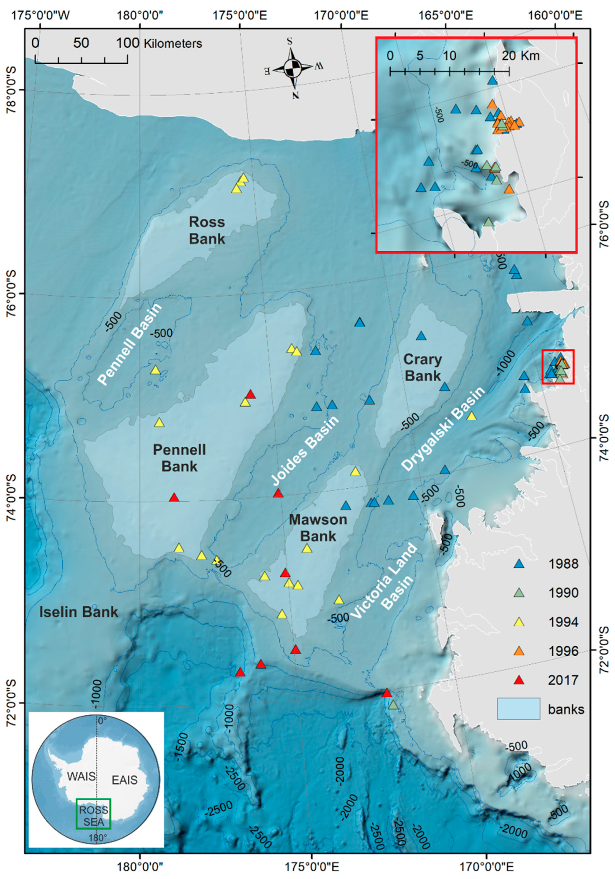
2.1. Study Area—Regional and Oceanographic Setting

The Ross Sea is located in the Pacific sector of the Southern Ocean, between Cape Colbeck at 158° W and Cape Adare at 170° E. On the southern side, it is bordered by the Ross Ice Shelf, at around 78.5° S. This broad ice shelf, which extends over nearly half of the continental shelf, is about 250 m thick on its northernmost side [60] and accounts for the 32% of the total Antarctica’s Ice Shelf volume [61]. The Ross Sea is characterized by a deep, irregular continental shelf with an average depth of 500 m and several shallow banks, separated by depressions. Most of these banks and depressions have a characteristic SSW/NNE orientation [62]. The eastern part of the Ross Sea has distinctly different characteristics from the western part in terms of physiography and seabed geology. The eastern region is characterized by broad troughs separated by low-relief ridges, while the western sector contains high relief banks and deep troughs [63]. The bottom topography in this area is rather irregular, with the ~500 m deep shelf isolated from the shore by the northeast-oriented 1200 m-deep Drygalski Basin [63].
The Ross Sea is the most productive sector of the Southern Ocean, and it is of critical importance to global biogeochemical cycles and in CO2 uptake. The region is characterized by strong vertical water mass exchanges that support higher trophic levels (e.g., penguins, whales, seals) [64].
The Drygalski Basin is a pathway for the cold, salty and dense shelf water (DSW) produced in the Terra Nova Bay, which flows towards the continental slope [65,66,67], and for warm and nutrient-rich water of circumpolar origin (Circumpolar Deep Water—CDW), flowing from the open ocean southwards onto the continental shelf [68,69,70,71,72]. The outflow of DSW and the intrusion of CDW onto the shelf in the Drygalski Basin are governed by tidal forcing [65,68]. Close to the shelf break, at the Drygalski mouth, Antarctic Bottom Water (AABW) is formed due to the tidal mixing of three different water masses DSW, CDW and Antarctic Surface Water (ASW) [66,68,73]. The freshening of the DSW and consequently of AABW formed in the Ross Sea have been observed since 1959 [74,75,76]. However, after 2014, the salinity of the Ross Sea AABW and of DSW has increased sharply and by 2018 had rebounded to values last observed in the mid–late 1990s. [77,78]. DSW is defined by a neutral density, (γn) > 28.27 kg m−3, and a potential temperature, <−1.85 °C, while CDW is identified by 28.00 < γn < 28.27 kg m−3 and a temperature maximum at intermediate depths [79].
Ice concentrations in the Ross Sea change dramatically during the different seasons, decreasing rapidly in austral spring recovering quickly in March. These seasonal changes in sea ice coverage, together with biological production, drive the seasonal variability of the Antarctic Surface Water (AASW) carbonate system [80]. Moreover, sea-ice melt water contributes to particulate iron (pFe) in the Ross Sea surface water at the sea ice edge on summer (e.g., [81]) and throughout a vast part of the Ross Sea that has recently been designated one of the world’s largest marine protected areas (CCAMLR Conservation Measure 91-05: Ross Sea Region Marine Protected Area. 2016 (https://www.ccamlr.org/en/measure-91-05-2016, last accessed on 25 May 2022).

2.2. Sediment of the Western Ross Sea Shelf

The dominant surface sediments of the deepest (>400 m) portions of the Ross Sea continental shelf are silt-rich siliceous muds with minor ice-rafted debris [82,83,84]. Unsorted mixtures of sand and gravel (residual glacial marine sediment) with various amounts of calcareous, bioclastic sand and gravel (consisting mainly of foraminiferal tests and fragments of bryozoans, barnacles, mollusks, corals and echinoderms) occur on offshore banks and on the outer continental shelf and upper slope where relatively strong currents sweep the sea floor [82,84].

2.3. Ostracods

The ninety surficial sediment samples analyzed for this study were collected during several oceanographic cruises (R/V Nathaniel B. Palmer cruises 1994, 1995; National Program of Antarctic Research—PNRA cruises 1988, 1990, 1991, 1996, 2017) (Figure 1). The gear used in the sampling, together with locations of the surficial samples collected in different oceanographic surveys, are reported in Table S1 in the Supplementary Materials.
The examined samples have been mainly collected by grab and dredge, and subsampling was carried out on board by distinguishing between the surficial layers and the remaining samples.
The samples were wet-sieved using a 50-µm mesh sieve, dried and weighed to determine the content of the sandy fraction. All living and dead ostracod specimens were dry picked, counted and identified, following the taxonomy of the Antarctic benthic ostracod systematic method [25,30,31,32,33,34,35,36,37,38,39,40,48,85]. The number of specimens refers to both valves and carapaces, i.e., one separated valve is considered to be one specimen and one articulated carapace is one specimen [25]. Following Brenchley and Harper [86] and Boomer et al. [87], a life assemblage was considered an autochthonous thanatocoenosis and a death assemblage (subjected to post-mortem transport and other processes, e.g., [88,89]) to be an allochthonous thanatocoenosis. In this sense, we considered autochthonous ostracod assemblages represented by living specimens or dead ones with left and right valves or complete carapaces of the adults together with their immature instars as life assemblages.
On the contrary, death assemblages (allochthonous thanatocoenosis) are represented by valves of adults without juveniles or juveniles without adults or with specimens showing evident signs of allochthonous taphocoenosis (fragmented and or abraded shells).
Only life (autochthonous) assemblages have been taken into account.
Ostracods discussed in the present paper are archived in the repository of the Department of Mathematics and Geosciences, University of Trieste.

2.4. Statistical Analysis

A similarity percentage (SIMPER) analysis defined the main taxa responsible for the differences between groups. These analyses were based on the Bray–Curtis dissimilarity, a measurement that does not take into account the absence of species but relies on the composition of assemblage and the relative abundances of taxa [91].
To characterize the biodiversity of assemblages, two faunal parameters were calculated: (1) species richness (Taxa_S), the number of species in each sample, and (2) the Shannon–index (Shannon_H), a measure of entropy that considers the distribution of taxa among the total number of specimens [92] (Table 1). Cluster analysis was run for the samples (Q-mode). The best results were reached using Ward’s method and the Bray and Curtis algorithm.
The redundancy analysis (RDA) [91,93] was applied to investigate the relationship between ostracod species and environmental variables through the samples. RDA was chosen after the application of the detrended correspondence analysis (DCA), as the gradient lengths were <4 standard deviations [94]. The total explained variation within the ostracod species data was partitioned among the three groups of environmental variables associated to depth, water temperature and salinity [95].
Multivariate analyses (Cluster and RDA analysis) on ostracod assemblages were performed using the Xlstat software Addinsoft (2020) (XLSTAT statistical and data analysis solution, New York, NY, USA; https://www.xlstat.com) and RStudio version 2021.9.0.351, 250 Northern Ave, Boston, MA 02210 844-448-1212, info@rstudio.com except for the calculation of SIMPER and of diversity indices, which was carried out using PAST software (PAlaeontological STatistic, version 4.07, https://www.nhm.uio.no/english/research/infrastructure/past/) [96]. Figures were produced using RStudio and processed with Inkscape software version 0.92. All ostracod taxa subjected to statistical analysis were previously standardized using the weight of the observed samples.

2.5. GIS Analysis

Predictive distribution maps for richness (i.e., the number of n° species in each sample) and total abundance (i.e., the number of specimens/g in each sample) were interpolated in GIS applying the spline method using barriers. The same method was used to interpolate salinity and temperature maps. The spline with barriers method is similar to the technique used in the spline tool, with the major difference being that this method honors discontinuities encoded in both the input barriers (Antarctica land and ice shelf) and the input point data. The spline with barriers tool applies a minimum curvature method, as implemented through a one-directional multigrid technique that moves from an initial coarse grid, initialized in this case to the average of the input data, through a series of finer grids until an approximation of a minimum curvature surface is produced at the desired row and column spacing (ESRI, 2021). The minimum curvature surface honors both the input point data and discontinuities encoded in the barriers. The deformation that is applied to each cell is calculated on the basis of a molecular summation [97] that compares the weighted summation of neighboring cells with the current value of a central target cell to calculate a new value for the target cell. The main difference between inverse distance weighting (IDW) and spline when using barriers, excluding the algorithm itself, is that IDW uses a “line of sight” approach and if a point cannot be “seen” because of a barrier, then it is not used to make the prediction. Spline with barriers instead weights the points based on the shortest distance around a barrier utilizing more points to make the prediction at that particular location. The cell size for the analysis is 500 m and no smoothing factor has been applied to the interpolation.

2.6. Oceanographic Data

Salinity, temperature and pressure data were acquired simultaneously with the sediment sampling activities during 17 Italian National Antarctic Research Programme (PNRA) expeditions from 1995 to 2019 (http://morsea.uniparthenope.it) and three Nathaniel B. Palmer expeditions in 2004, 2013 and 2018, as part of the ANSLOPE (http://ocp.ldeo.columbia.edu/res/div/ocp/projects/anslope/Data.html.), TRACERS (https://doi.org/10.1594/IEDA/320068) and CICLOPS (https://www.bco-dmo.org/dataset/783911) projects, respectively. The data were obtained using a CTD Sea-Bird Electronics SBE 9/11+. The CTD was equipped with dual temperature-conductivity sensors flushed by a pump at a constant rate. Calibrations were performed before and after the cruises. Hydrographic data were corrected and processed according to standard procedures [98]. The maps in Figure 2A,B were obtained by averaging the salinity and temperature in the bottom 10 dbar at each station.

3. Results

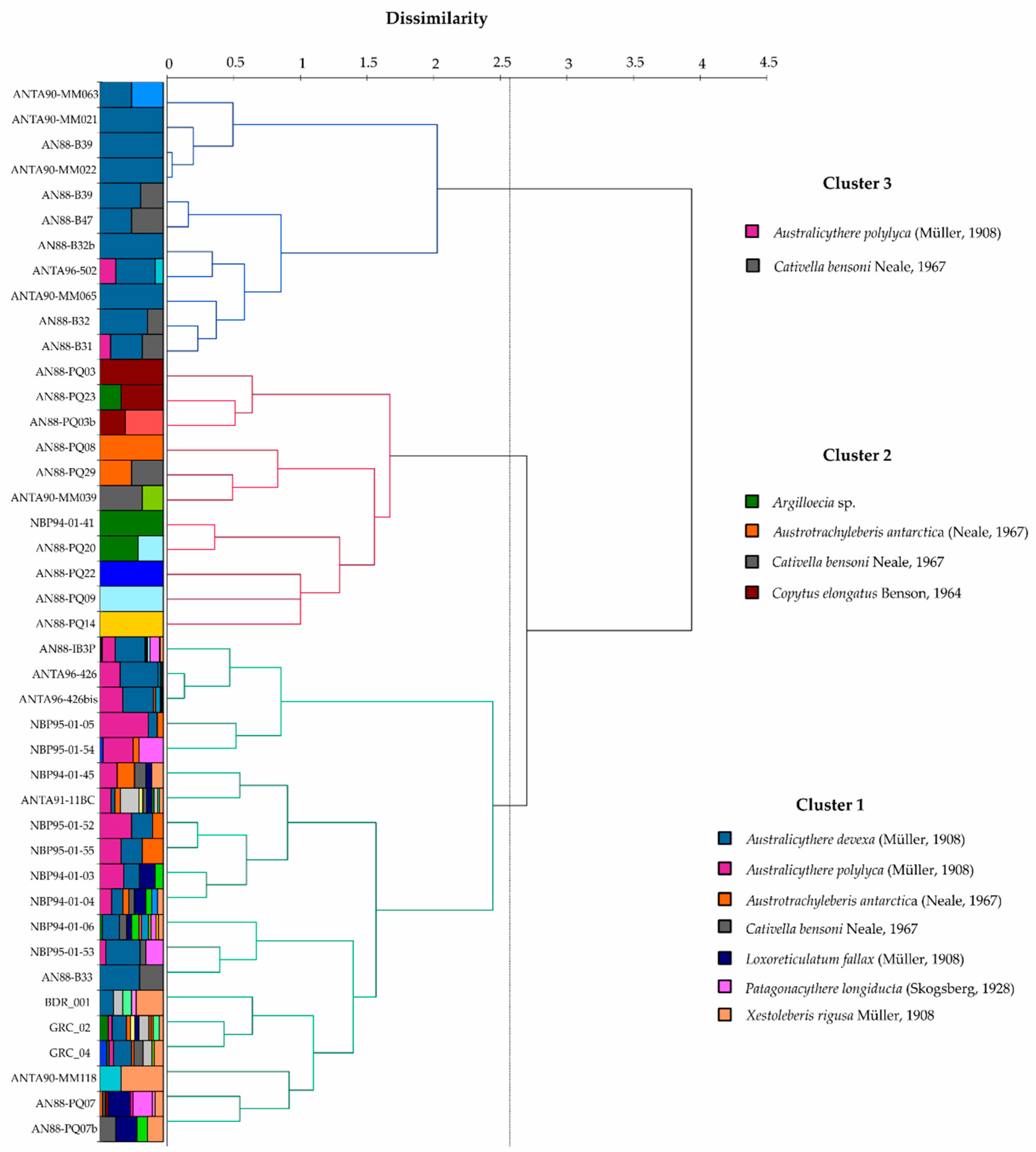
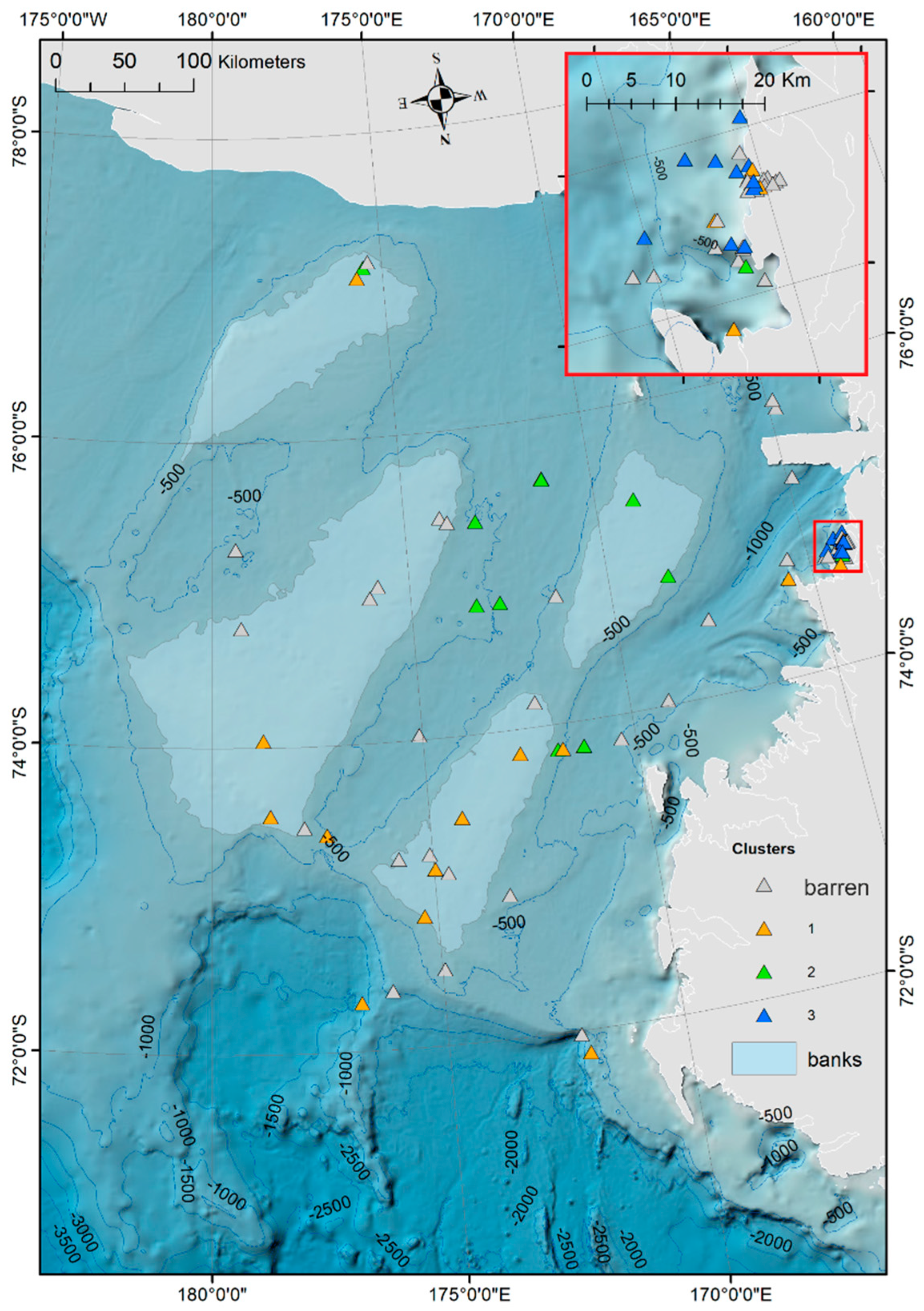
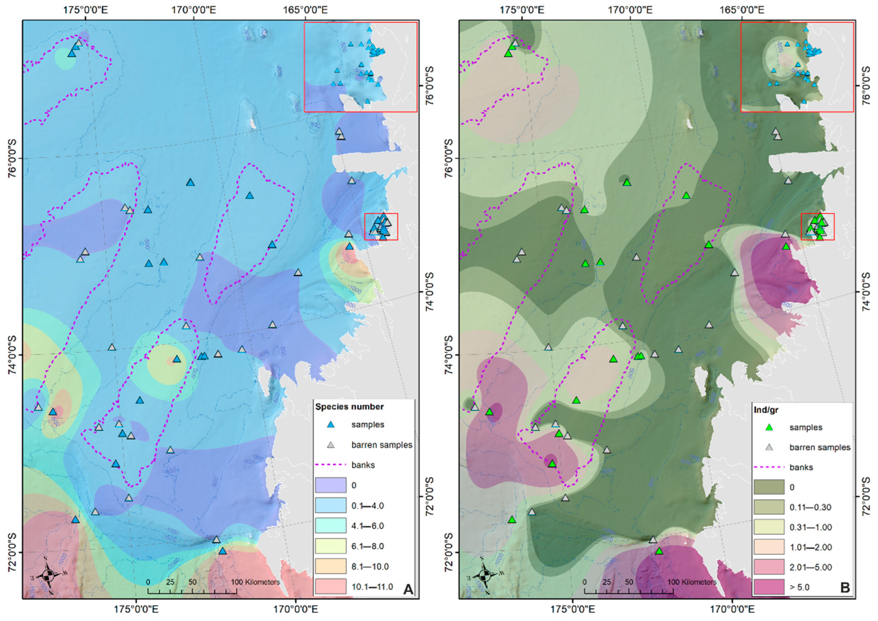
Ostracod Assemblages in the Western Ross Sea Shelf

Among the 90 surface samples examined, 42 contained an ostracod fauna, which consisted in 28 species, and 6 species were recorded in open nomenclature (Table S1 in the Supplementary Materials). The 48 samples without ostracods or with valves showing evident signs of allochthonous taphocoenosis (fragmented and or abraded shells) were mainly collected in the southernmost and central areas of the WRSS, in the northern part of the Drygalski and Victoria Land Basin. The Q-mode cluster analysis performed on the ostracod assemblages of the WRSS identified three groups of samples (Figure 3) characterized by increasing abundance e richness values (from Cluster 3 to Cluster 1, respectively) with the highest values of ostracod fauna recorded in the northwestern area of the WRSS (shelf break east to Cape Adare) on the outer shelf, on the banks and in the Terra Nova Bay (TNB) and in a nearby area. High values were also recorded in the Ross Bank area (Figure 4).
Within the Cluster 1 the dominant species are: Australicythere devexa (Müller, 1908), Australicythere polylyca (Müller, 1908), Austrotrachyleberis antarctica (Neale, 1967), Cativella bensoni Neale, 1967, Loxoreticulatum fallax (Müller, 1908), Patagonacythere longiducta (Skogsberg, 1928), Xestoleberis rigusa Müller, 1908; in the Cluster 2: Argilloecia sp., Austrotrachyleberis antarctica (Neale, 1967), Cativella bensoni Neale, 1967, Copytus elongatus Benson, 1964; and in the Cluster 3: Australicythere polylyca (Müller, 1908), Cativella bensoni Neale, 1967 (Figure A1, Figure A2 and Figure A3).
SIMPER analysis showed that more than 60% of the difference between clusters is defined by Australicythere polylyca (23.84% relative contribution), Australicythere devexa (20.04%), Xestoleberis rigusa (8.63%), Loxoreticulatum fallax (6.62%), Cativella bensoni (6.56%) and Austrotrachyleberis antarctica (6.42%), followed by lower contributions of Patagonacythere longiducta (5.69%) and Argilloecia sp. (3.66%) (Table 2).
The Shannon_H values range between 0 (samples NBP94-01-41, AN88-B32b, AN88-B39b, AN88-PQ03, AN88-PQ08, AN88-PQ09, AN88-PQ14, AN88-PQ22, ANTA90-MM021, ANTA90-MM022 and ANTA90-MM065) and 2.23 (sample GRC_02). High values were also recorded in NBP94-01-06 (2.19) and ANTA91-11BC (2.13). The overall Shannon_H value is not very high and reveals an ostracod assemblage characterized by low qualitative and quantitative values (Figure 5). The redundancy analysis (RDA) was performed in order to link the species found in the surface sediments of the WRSS with the environmental variables analyzed (depth, salinity, temperature). The first two axes explain 10.50% of the observed variance, while first three axes explain 12.00%. Salinity plays a key role on site dispersion along the first axis; depth and water temperature appear to be correlated to both first and second axes. There is a positive correlation between the increasing ostracods abundance and richness values and the salinity parameter; similarly, temperature shows a comparable tendency with a positive correlation mainly with A. devexa, A. antarctica, C. fallax, C. antarcticum, P. longiducta and X. rigusa; depth is positively correlated with Argilloecia sp., B. dubia, B. simplex, C. bensoni and Copytus elongatus. A. polylyca does not show any correlation with the examined variables (Figure 6).

4. Discussion

4.1. Analysis of the Ostracod Assemblages in Respect to WRSS Bathymetric Zones

Calcareous organisms, such as calcitic ostracods, represent a valuable paleoenvironmental, paleoclimatic, palaeoceanographic and biostratigraphic indicator [2,3,4,5,6]. When comparing living and fossil ostracods, it is vital to understand the potential range of similarity and difference between a living population and the fossil assemblages recovered from a sediment series (cores, boreholes), which can range from something close to the original live fauna (thanatocoenosis—if in situ, i.e., autochthonous) to allochthonus assemblages that have been subjected to varying degrees of transport with consequent sorting and loss (taphocoenosis) [99].
The analysis carried out on the ostracod association found in surface sediments from the WRSS, for the first time provided the opportunity to analyze distribution patterns in relation to data variables (temperature, salinity) documented from numerous oceanographic cruises organized by the PNRA since the 1990s. In particular, it is possible to correlate the species found with precise ranges (maximum and minimum) of temperature, salinity and depth, thus providing new insight into the distribution of species in relation to the above-mentioned variables (Figure 7, Table S2).
We recorded a high proportion of previously undiscovered ostracod diffusions in the WRSS, as found in Atlantic Sector of the Southern Ocean by [26]. This is not surprising because of the very low number of previous studies in the Ross Sea Area [22,40,41,42,43] and given the wide and deep continental shelf.
Moreover, in agreement with [22,26], the low proportion of the ostracod richness and abundance (i.e., n° specimen/g) in the WRSS, in contrast with its considerable area, also suggest a high level of yet undiscovered ostracod biodiversity, probably due to inadequate sampling and the level of geographical cover, with a large number of new species probably still to be discovered ([22], p. 143) (Figure 8A,B).
The most representative species, as defined by SIMPER analyses, show a preferential distribution in the well-defined areas of the WRSS. In particular, A. polylyca, the most abundant taxon within WRSS fauna, was found in the south-western part of the WRSS (Drygalski Basin), in the northern part of the Joides Basin and at the shelf break east of Cape Adare (Figure 9A). This endemic taxon was widely recorded from the modern Antarctic region [25,26]. Another finding of interest is the occurrence of this thaerocytherid species, common in Antarctic shallow waters (48 to 464 m), in the eastern Weddell Sea at a depth of 1030 m, possibly indicating its submergence from the Antarctic shelf [23]. Additionally, the highest abundance of living specimens of this taxon was recorded in the deep areas of continental shelf and slope, showing that this species may be able to migrate vertically throughout the continental margin in a relatively short time [22]. Recently, [26] identified the genus Australicythere in the continental slope of Antarctica and adjacent abyssal plain (3631 m). We also noted that A. polylyca is the only species that does not have a correlation with the variables examined. Likewise, our study documents the occurrence of A. polylyca at varying depths of the Ross Sea shelf (from 79 to 723 m), highlighting the possible eurybathic characteristics of this species, which may have survived past glaciations on the slope or deeper.
Australicythere devexa, the second-most abundant species in the WRSS surficial sediments, shows a distribution comparable to A. polylyca, except for its occurrence in the southern part of the WRSS (Ross Bank) (Figure 9B). This taxon is extant in southern-most South America [100,101], South Georgia [30,35] and throughout the Antarctic [37]. Its depth range until now has been relatively restricted (50–385 m), with the exception of the few littoral sites mentioned by [101,102] in the Strait of Magellan. The wide modern distribution in southern South America may be linked by South American origin or by an early migration from Antarctica. Another factor of this broad geographical distribution is likely its adaptation to a wide range of water depths, including the littoral zone and relatively deep water [25,101,102]. Considering this, we noted the presence of A. devexa in a wide depth range from 220 to 723 at the shelf break area, on the Ross Bank and in TNB and nearby area seabed. X. rigusa, L. fallax, C. bensoni, A. antarctica and P. longiducta with lesser abundance values show a less extensive diffusion in the WRSS area with highest values recorded mainly at the shelf break, in the northern part of the Joides Basin, in the Ross Bank area, in the TNB and in a nearby area.
Xestoleberis rigusa was recorded by [39] from the west coast of the Antarctic Peninsula (Paradise Bay) at a water depth of 2 m, and in Halley Bay from a depth of 206 m. Hartmann [37] recorded X. rigusa off Elephant Island, Bransfield Strait and the Antarctic Peninsula (Joinville, d’Urville, Lavoisier and Adelaide Islands) with the depth range 130–385 m. Finally, ref. [24] reported the occurrence of X. rigusa with a water-depth range 34–450 m in Admiralty Bay (Antarctic Peninsula). L. fallax, previously documented from Antarctic waters by [38], was also recorded in the Lützow-Holm Bay [25], in Admiralty Bay [24,103] and from the shallow Kerguelen Plateau [104], at a depth range 110–280 m. In the Ross Sea, X. rigusa and L. fallax were found mainly near the shelf break, in the northern part of the Joides Basin, in the Ross Bank and in TNB and nearby area seabed (Figure 10A,B).
Cativella bensoni was often reported from the modern Antarctic Peninsula (Halley Bay) [38] and from the Strait of Magellan [101]. C. bensoni is also recorded from >1000 m depth around the Kerguelen Islands by [104], while in Antarctica proper it occurs below ~450 m [25,48]. We recorded the higher density of C. bensoni at the shelf break and in the northern part of the Joides Basin (Figure 11A).
Austrotrachyleberis antarctica was originally described as Robertsonites antarctica from Halley Bay [38]. It has since been recorded by [37] in South Georgia and in several areas in the northern Antarctic Peninsula and in the Strait of Magellan between 1–456 m [101]. A. antarctica is mainly localized at the shelf break and in the Ross Bank area (Figure 11B). Finally, Patagonacythere longiducta was found to be widespread in the Antarctic and Subantarctic areas in shallow waters [24,25,39], while in WRSS it is mainly found in and near TNB (Figure 12). In summary, all five taxa show a wide depth range of 47–723 m, except for P. longiducta, whose depth appears more constrained (220–509 m) (Figure 7, Table S2).

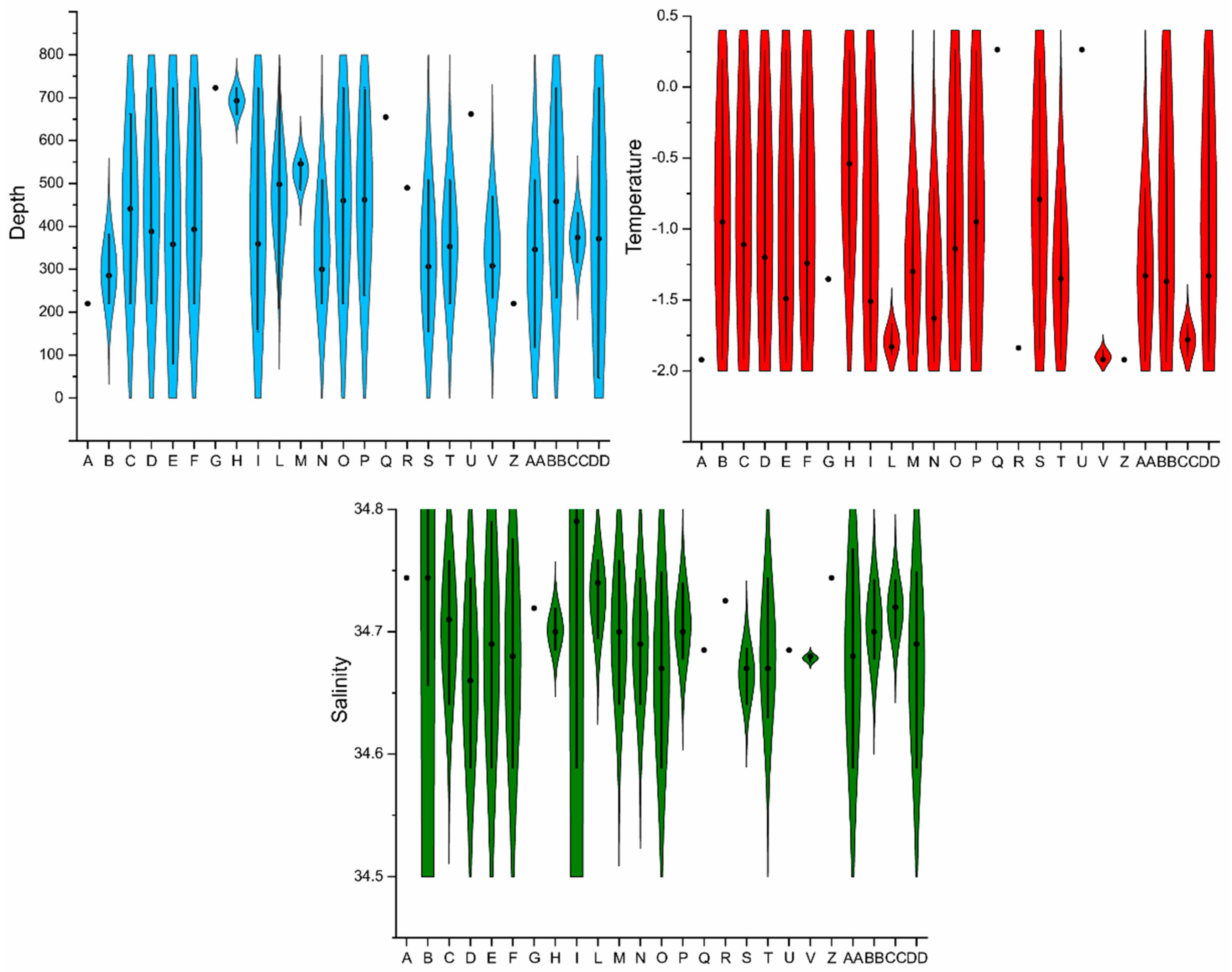
4.2. Distribution of Autochthonous Ostracod Assemblages in Response to the Oceanographic Settings

The results provided here yield additional knowledge on recent ostracod assemblages from several areas of the WRSS. These assemblages occur at different water depths and in different oceanographic settings and provide modern analogues useful for the reconstruction of the geological record (Figure 7, Table S2). Our results also indicate that water depth may not be an obstacle to species dissemination, as also reported by [19]. Ostracod richness and abundance are more connected to low salinity and higher temperature values (i.e., CDW water–mass characteristics), as reported by [25] in Lützow-Holm Bay, east Antarctica.
Ostracods bathymetric occurrence was analyzed from the shallow to the deep continental shelf (8–520 m) at King George Island (Antarctic Peninsula) by [24] and in the deep continental shelf and shallow slope (350–870 m) of Lützow-Holm Bay, east Antarctica [25]. These authors reported distinct ostracod faunas living in different depth zones from these areas from the Southern Ocean [26]. Similarly, our results recorded the distribution of WRSS ostracod assemblages in a wide range of water depths from shallow continental shelf to shallow slope.
Ostracods might have colonized diverse shelf environments in the Ross Sea during the last glacial age, possibly surviving within ice-free refugia, or, alternatively, below the ice shelf, as recorded by recent micropaleontological results [59] from studies of benthic communities living under the ice shelves [105]. Most ostracods are deposit feeders and could potentially have survived in such environments [26].
Recent studies [60,81,106] reported the importance of sea ice conditions and their influence on productivity and the flux of organic material to the seafloor [107,108,109] as a driver of benthic community structure and function (e.g., [110,111]), even at depths far below the surface [112]. Similarly, the mechanisms of nutrient distribution and sediment supply in the WRSS are primarily related to the circulation of water masses and the different oceanographic regimes affecting the Ross Sea shelf seafloor.
Castagno et al. ([68,84] and references therein) verified how CDW, a relatively warm water mass that impacts onto the Ross Sea continental shelf at intermediate and surface levels of the water column and transports fine silt and diatom fragments along the eastern sides of troughs on the middle and inner continental shelf where lower current velocities allow these sediments to settle. This winnowing on the outer shelf and banks results in more conditions that are more conducive for calcite preservation than the inner shelf [113].
Recent studies on the living and dead benthic foraminiferal distributions in the Ross Sea areas [60,114] confirmed the importance of the influence of CDW in preserving calcareous taxa, especially considering that the corrosive HSSW is mitigated by the contact with other water masses [68]. Equally, the nutrients distributed by CDW allows other carbonate organisms to thrive [54,115], as recorded by the high number of cold-water bioclastic carbonates (bryozoans, barnacles and corals) detected on the outer shelf and on banks in the northwestern Ross Sea [84]. In this sense, our data fit well with water masses rich in nutrients (CDW) as possible main factors controlling the nutrient intakes within the Ross Sea area and ostracods diffusion. In addition, we observed rising values of the ostracod density and richness in the Terra Nova Bay and in a nearby area where warm water, rich from circumpolar origin (CDW), flows from the open ocean southwards onto the continental shelf ([68] and the references therein) (Figure 2A,B). Additionally, ref. [81], investigating the distribution of particulate Fe (pFe), suspended particulate matter (SPM) and other particulate trace metals in TNB to highlight the spatial heterogeneity of both SPM and particulate metals concentrations in the water masses, thus confirming that biogenic iron may significantly contribute to the bioavailable iron pool, sustaining both primary production and higher ostracod fauna richness in this area.
The findings of [101,102] partially confirm the possible link between ostracods presence to oceanographic settings with the recovery of several normally deeper water ostracod species (A. antarctica, A. devexa and B. simplex) from medium and even littoral depths in the Strait of Magellan, probably accounting for the coastal upwelling of very cold, deep water. In this regard, our results underscore the importance of water mass properties and oceanographic circulation to the dispersal, distribution and flux of the surface derived food sources (e.g., [116]) as main drivers in WRSS ostracod distribution [19]. The results show that the meiofaunal distribution in the Ross Sea shelf is largely dependent upon the amounts of utilizable organic matter in sediments [117], which in turn are largely controlled by main Ross Sea water masses [68].
Finally, given the absence of ostracod fauna recorded in 48 of the 90 samples observed over a wide depth range, further investigation will be required for better analyze the possible relationship between carbonate dissolution effects in the Ross Sea area and the presence/absence of ostracod specimens.
In this sense, the little research carried out on the distribution of benthic foraminifera [118,119,120] revealed that the Ross Sea contains typical Antarctic foraminifera fauna dominated by agglutinated taxa, underlining at the same time how the ice cover, the activity of bottom currents and the intensity of primary production are factors influencing the distribution of benthic foraminifera. Moreover, the conservation of calcareous foraminifera also depends on the CCD that in the Ross Sea is shallower because of the low temperature, the high CO2 content and the low surface primary productivity, which are reduced, owing to the presence of a thick pack-ice.
In addition, Capotondi et al., [60,114], in analyzing the foraminiferal faunas in the Joides basin, demonstrated how high productivity, together with high organic carbon content in surface sediments and oxic conditions at the sediment–water interface, could trigger carbonate dissolution for increasing dissolved CO2, thus favoring the agglutinated taxa. In the same way, the degradation of organic matter via a synergistic effect with high pressure and low temperature can occur, amplifying the corrosive effect at the investigated site [121].
In contrast, ref. [122] recognized the ability of ostracods to thrive below the CCD with the high number of specimens collected in the Kuril-Kamchatka Trench at depths far below the CCD. With respect to future scenarios related to global warming and ocean acidification, calcitic organisms like ostracods could indeed prove to be more resilient than other calcifiers. To test this hypothesis, however, there is the need to improve the scant knowledge concerning the physiology of these crustaceans.

5. Conclusions

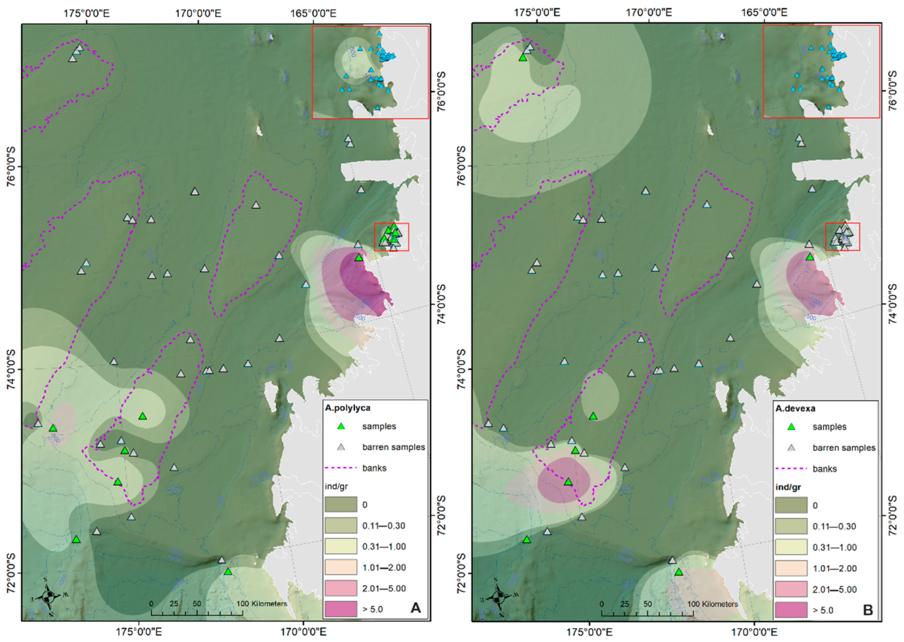
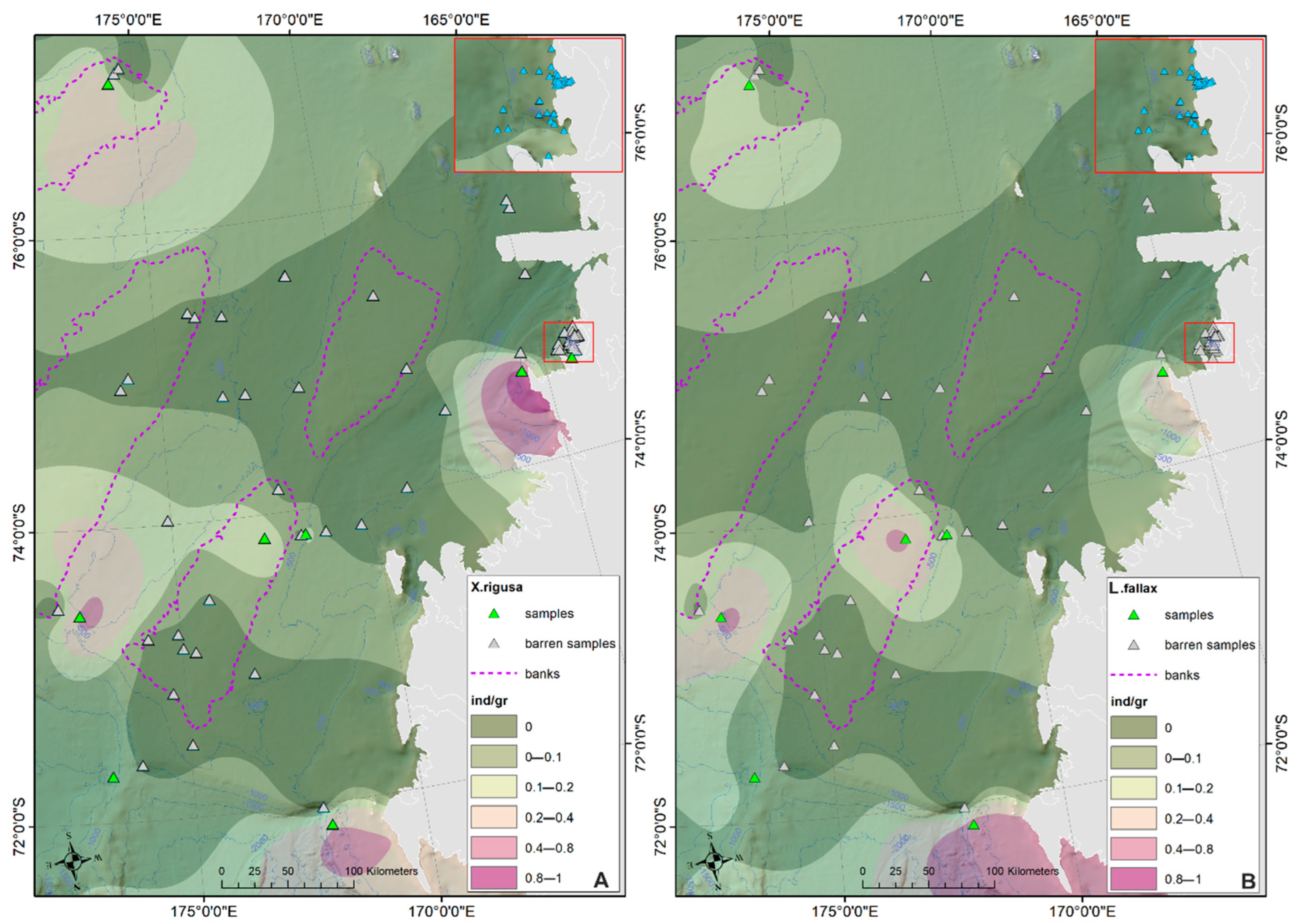
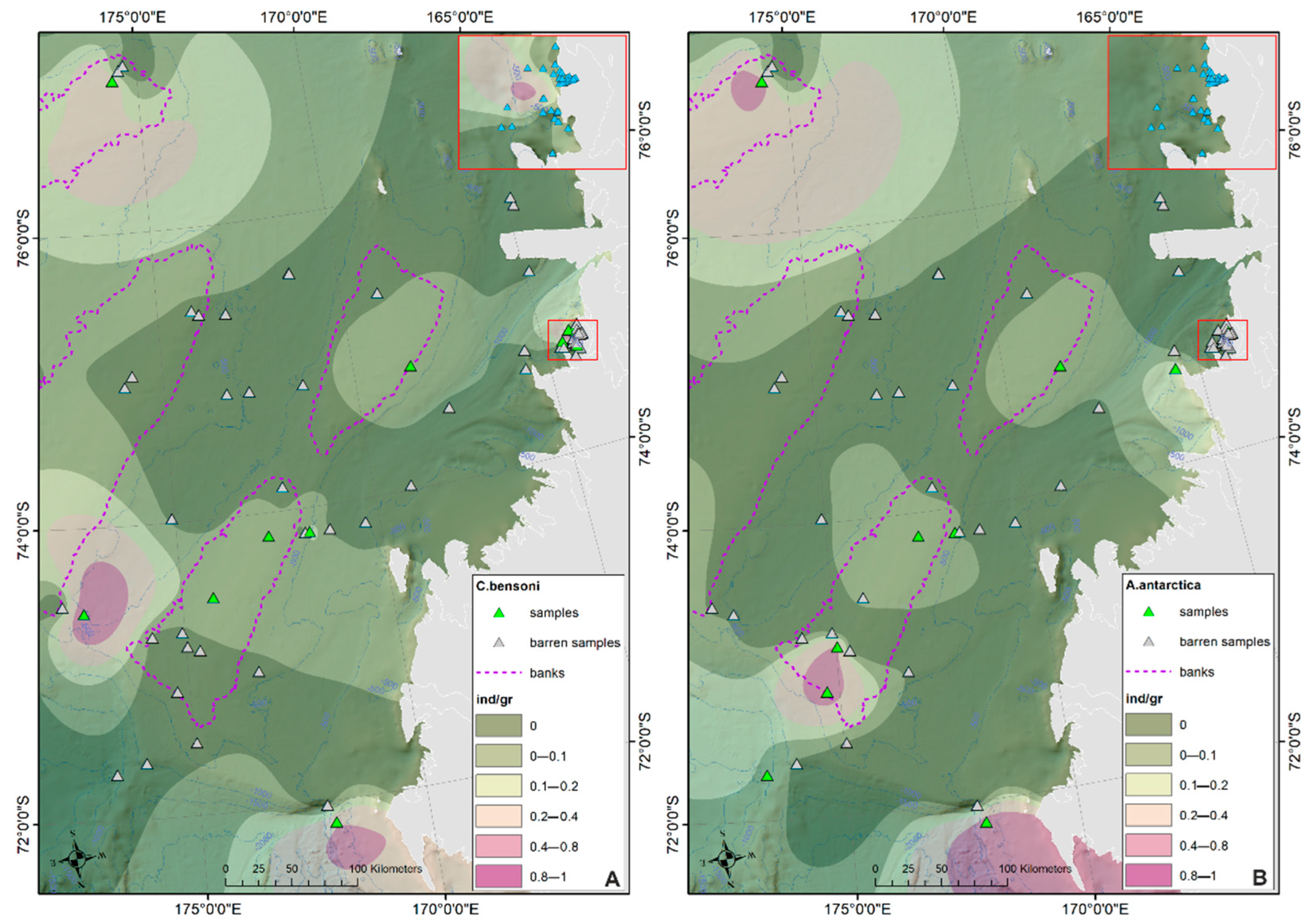
  • The prevalent ostracod assemblages in WRSS are represented by Australicythere polylyca, Australicythere devexa, Xestoleberis rigusa, Loxoreticulatum fallax, Cativella bensoni, Austrotrachyleberis antarctica and Patagonacythere longiducta; all these species are able to colonize different shelf environments along an extensive range of water depths. These characteristics may have served as a potential source for shelf recolonization after the last glacial phase.
  • Salinity and temperature are the oceanographic variables that better explain the main variance in the examined samples; in particular, the dominant ostracod species are positively correlated with temperature, outlining a possible close link between diffusion of the ostracod assemblages and CDW (a relatively warm water mass that flows onto the Ross Sea shelf at intermediate and surface levels), as a major factor controlling the nutrient intakes within the Ross Sea.
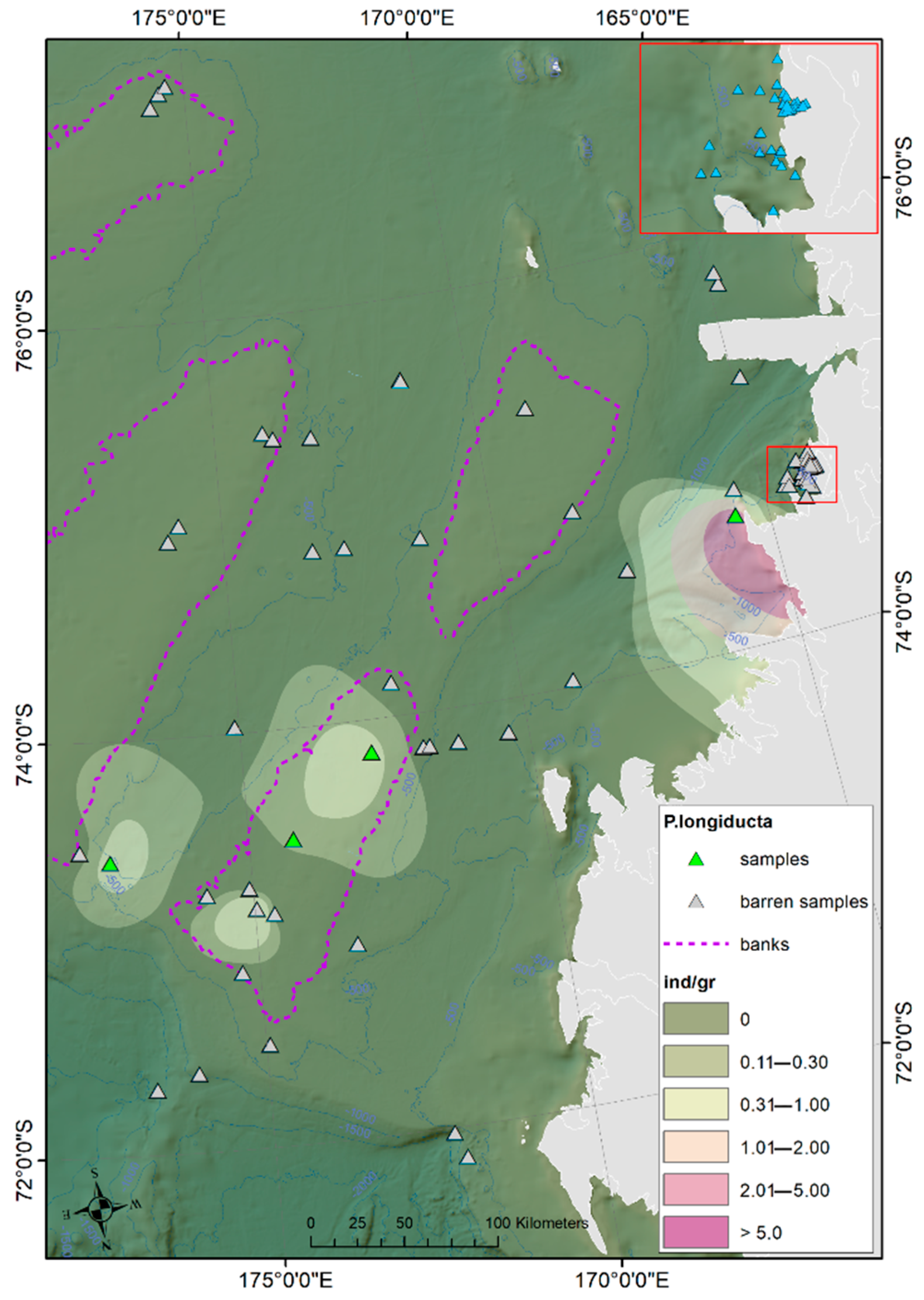
  • Rising values of the ostracod assemblages were also recorded in and particularly north of the Terra Nova Bay, where nutrient enrichment is derived from warm water of circumpolar origin (Circumpolar Deep water—CDW) flowing from the open ocean southwards onto the continental shelf. Recent analyses have shown an increase in primary production supported by biogenic iron in the same area.

Supplementary Materials

The following are available online at https://www.mdpi.com/article/10.3390/min12080937/s1, Table S1: list of recognized autochthonous ostracod species, as number of specimen/g, recovered in the WRSS surficial sediments. Shannon index (Shannon_H), species richness and total abundance (n° of specimens/g) have been added. Green colored cells identify species found in biocoenosis in the WRSS; Table S2: Depth, temperature and salinity ranges (Min., Max., Average values) for the ostracod species recovered in the Western Ross Sea Shelf area. The dominant species are reported in green color.

Author Contributions

Conceptualization, G.S. and M.T.; investigation, G.S., J.B.A., P.C., P.F., P.M. and M.T.; writing—original draft preparation, G.S., M.T. and J.B.A.; writing— review and editing, G.S., P.C., P.F., P.M., M.B., M.F., M.T. and J.B.A.; formal analysis, G.S., P.C., P.F. and M.T.; data curation, G.S., P.C., P.F., M.B. and M.F.; methodology, G.S., P.C., P.F., M.B. and M.T.; funding acquisition, G.S. and P.M. All authors have read and agreed to the published version of the manuscript.

Funding

This research was supported by GRACEFUL (grant No. PNRA16_00069, 11 October 2017–10 October 2020) and IODP374_28 (grant No. PNRA18_00233, 12 April 2019) projects and funded by the Italian National Antarctic Research Program.

Acknowledgments

Thanks to Mauro Bussi, Cristiano Landucci and Gualtiero Tujach for support in laboratory activities. We thank Karolyn Close for kindly reading the manuscript and revising the English language in a preliminary version of the manuscript. This is Ismar-CNR, Bologna scientific contribution n. 2066.

Conflicts of Interest

The authors declare no conflict of interest.

Appendix A

Figure A1. 1—Antarcticythere laevior. Lateral exterior view, left valve; 2—Australicythere devexa. Lateral exterior view, right valve; 3—Australicythere polylyca. Lateral exterior view, left valve; 4—Austrotrachyleberis antarctica. Lateral exterior view, left valve; 5—Bairdoppilata simplex. Lateral exterior view, right valve; 6—Bythoceratina dubia. Lateral exterior view, left valve; 7—Cativella bensoni. Lateral exterior view, right valve.
Minerals 12 00937 g0a1
Figure A2. 1—Cytheropteron antarcticum. Lateral exterior view, left valve; 2—Cytheropteron sp. Lateral exterior view, left valve; 3—Echinocythereis sp. Lateral exterior view, left valve; 4—Krithe (Austrokrithe) magna. Lateral exterior view, right valve; 5—Loxoreticulatum fallax. Lateral exterior view, left valve; 6—Macropyxis similis. Lateral exterior view, right valve; 7—Nodoconcha minuta. Lateral exterior view, right valve; 8—Patagonacythere longiducta. Lateral exterior view, left valve.
Minerals 12 00937 g0a2
Figure A3. 1—Polycope sp. Lateral exterior view, left valve; 2—Pseudocythere aff. P. caudata. Lateral exterior view, left valve; 3—Sclerochilus (Praesclerochilus) antarcticus. Lateral exterior view, right valve; 4—Sclerochilus (Praesclerochilus) reniformis. Lateral exterior view, right valve; 5—Semicytherura sp. Lateral exterior view, right valve; 6—Xestoleberis rigusa. Lateral exterior view, right valve.
Minerals 12 00937 g0a3

References

  1. Yamaguchi, T. Valve calcification in the evolutionary history of marine ostracodes (Ostracoda). J. Crustacean Biol. 2018, 39, 253–260. [Google Scholar] [CrossRef]
  2. Benson, R.H. Ostracods and Palaeoceanography. Ostracoda in the Earth Sciences. In Proceedings of the 11th International Symposium on Ostracoda, Warrnambool, Australia, 8–12 July 1991; De Deckker, P., Colin, J.P., Peypouquet, J.P., Eds.; A.A. Balkema: Rotterdam, The Netherlands, 1988; pp. 1–26. [Google Scholar]
  3. Cronin, T.M.; Holtz, T.R.; Whatley, R.C. Quaternary paleoceanography of the deep Arctic Ocean based on quantitative analysis of Ostracoda. Mar. Geol 1994, 119, 305–332. [Google Scholar] [CrossRef]
  4. Cronin, T.M.; De Martino, D.M.; Dwyer, G.S.; Rodriguez-Lazaro, J. Deep-sea ostracode species diversity: Response to late Quaternary climate change. Mar. Micropaleontol. 1999, 37, 231–249. [Google Scholar] [CrossRef] [Green Version]
  5. Yasuhara, M.; Cronin, T.M.; Hunt, G.; Hodell, D.A. Deep–sea ostracods from the South Atlantic sector of the Southern Ocean during the Last 370,000 years. J. Paleontol. 2009, 83, 914–930. [Google Scholar] [CrossRef]
  6. Rodriguez-Lazaro, J.; Ruiz-Munõz, F. A General Introduction to Ostracods: Morphology, Distribution, Fossil Record and Applications. Dev. Quat. Sci. 2012, 17, 1–14. [Google Scholar] [CrossRef]
  7. Cronin, T.M.; Raymo, M.E. Orbital forcing of deep-sea benthic species diversity. Nature 1997, 385, 624–627. [Google Scholar] [CrossRef]
  8. Cronin, T.; Dwyer, G.; Baker, P.A.; Rodriguez Lazaro, J.; Demartino, D.M. Orbital and suborbital variability in North Atlantic bottom water temperature obtained from deep-sea ostracode Mg/Ca ratios. Palaeogeogr. Palaeoclimatol. Palaeoecol. 2000, 162, 45–57. [Google Scholar] [CrossRef] [Green Version]
  9. Cronin, T.M.; Dwyer, G.S.; Farmer, J.; Bauch, H.A.; Spielhagen, R.F.; Jakobsson, M.; Nilsson, J.; Briggs, W.M., Jr.; Stepanova, A. Deep Arctic Ocean warming during the last glacial cycle. Nat. Geosci. 2012, 5, 631–634. [Google Scholar] [CrossRef]
  10. Rodriguez Lazaro, J.; Cronin, T. Quaternary glacial and deglacial Krithe (Ostracoda) in the thermocline of the Little Bahama Bank (NW Atlantic): Palaeoceanographic implications. Palaeogeogr. Palaeoclimatol. Palaeoecol. 1999, 152, 339–364. [Google Scholar] [CrossRef]
  11. Didié, C.; Bauch, H.A.; Helmke, J.P. Late Quaternary deep-sea ostracodes in the polar and subpolar North Atlantic: Paleoecological and paleoenvironmental implications. Palaeogeogr. Palaeoclimatol. Palaeoecol. 2002, 184, 195–212. [Google Scholar] [CrossRef]
  12. Dwyer, G.S.; Cronin, T.M.; Baker, P.A.; Rodriguez Lazaro, J. Changes in North Atlantic deep-sea temperature during climatic fluctuations of the last 25,000 years based on ostracode Mg/Ca ratios. Geochem. Geophys. Geosyst. 2000, 1, 17. [Google Scholar] [CrossRef] [Green Version]
  13. Bodergat, A.M. Les Ostracodes, témoins de leur environnement: Approche chimique et écologique en milieu lagunaire et océanique. Doc. Lab. Géol. Fac. Sci. Lyon. 1983, 88, 1–246. [Google Scholar]
  14. De Deckker, P. Ostracod paleoecology. The ostracoda: Application in quaternary research. Am. Geophys. Union Wash. 2002, 131, 121–134. [Google Scholar]
  15. Decrouy, L. Biological and environmental controls on isotopes in ostracod shells. In Ostracoda as Proxies for Quaternary Climate Change. Developments in Quaternary Science; Horne, D.J., Holmes, J., Rodriguez-Lazaro, J., Viehberg, F.A., Eds.; Elsevier: Amsterdam, The Netherlands, 2012; Volume 17, pp. 165–181. [Google Scholar] [CrossRef]
  16. Dingle, R.V. Insular endemism in Recent Southern Ocean benthic Ostracoda from Marion Island: Paleozoogeographical and evolutionary implications. Rev. Esp. Micropaleontol. 2002, 34, 215–233. [Google Scholar]
  17. Dingle, R.V. Recent Subantarctic benthic ostracod faunas from the Marion and Prince Edward Islands Archipelago, Southern Ocean. Rev. Esp. Micropaleontol. 2003, 35, 119–155. [Google Scholar]
  18. Kaiser, S.; Griffiths, H.J.; Barnes, D.K.A.; Brandão, S.N.; Brandt, A.; O’Brien, P.E. Is there a distinct continental slope fauna in the Antarctic? Deep Sea Res. Part II Top. Stud. Oceanogr. 2011, 58, 91–104. [Google Scholar] [CrossRef]
  19. Brandão, S.N.; Vital, H.; Brandt, A. Southern Polar Front macroecological and biogeographical insights gained from benthic Ostracoda. Deep Sea Res. Part II Top. Stud. Oceanogr. 2014, 108, 33–50. [Google Scholar] [CrossRef]
  20. Ayress, M.; Neil, H.; Passlow, V.; Swanson, K.M. Benthonic ostracods and deep watermasses: A qualitative comparison of southwest Pacific, southern and Atlantic Oceans. Palaeogeogr. Palaeoclimatol. Palaeoecol. 1997, 131, 287–302. [Google Scholar] [CrossRef]
  21. Brandão, S.N.; Horne, D.V. The Platycopid Signal of oxygen depletion in the ocean: A critical evaluation of the evidence from modern ostracod biology, ecology and depth distribution. Paleogeogr. Paleoclimatol. Paleoecol. 2009, 283, 126–133. [Google Scholar] [CrossRef]
  22. Brandão, S.N.; Dingle, R.V.; De Broyer, C. Biogeographic Atlas of the Southern Ocean; Koubbi, P., Griffiths, H.J., Raymond, B., d’Udekem d’Acoz, C., Van de Putte, A.P., Danis, B., David, B., Grant., S., Gutt, J., Eds.; Scientific Committee on Antarctic Research: Cambridge, UK, 2014; pp. 142–148. [Google Scholar]
  23. Brandt, A.; Gooday, A.; Brandão, S.; Brix, S.; Brökeland, W.; Cedhagen, T.; Choudhury, M.; Cornelius, N.; Danis, B.; De Mesel, I.; et al. First insights into the biodiversity and biogeography of the Southern Ocean deep sea. Nature 2007, 447, 307–311. [Google Scholar] [CrossRef]
  24. Majewski, W.; Olempska, E. Recent ostracods from Admiralty Bay, King George Island, West Antarctica. Pol. Polar Res. 2005, 26, 13–36. [Google Scholar]
  25. Yasuhara, M.; Kato, M.; Ikeya, N.; Seto, K. Modern benthic ostracodes from Lützow-Holm Bay, East Antarctica: Paleoceanographic, paleobiogeographic, and evolutionary significance. Micropaleontology 2007, 53, 469–496. [Google Scholar] [CrossRef]
  26. Brandão, S.N.; Saeedi, H.; Brandt, A. Macroecology of Southern Ocean benthic Ostracoda (Crustacea) from the continental margin and abyss. Zool. J. Linn. Soc. 2022, 194, 226–255. [Google Scholar] [CrossRef]
  27. Brandão, S.N.; Sauer, J.; Schön, I. Circumantarctic distribution in Southern Ocean benthos? A genetic test using the genus Macroscapha (Crustacea, Ostracoda) as a model. Mol. Phylogenet. Evolut. 2010, 55, 1055–1069. [Google Scholar] [CrossRef] [PubMed]
  28. Anderson, J.B. Factors controlling CaCO3 dissolution in the Weddell Sea from foraminiferal distribution patterns. Mar. Geol. 1975, 19, 315–332. [Google Scholar] [CrossRef]
  29. Rao, C.P. Modern Carbonates: Tropical, Temperate, Polar. Ph.D. Thesis, University of Tasmania, Hobbart, Tasmania, 1996. [Google Scholar]
  30. Hartmann, G. Antarktische benthische Ostracodan III. Auswertung der Reise des FFS “Walther Herwig” 68/1. 3. Teil: Süd-Orkney-Inseln. Mitt. Aus. Dem. Hambg. Zool. Mus. Und. Institut. 1988, 85, 141–162. [Google Scholar]
  31. Hartmann, G. Antarktische benthische Ostracodan IV. Auswertung der wahrend der Reise von FFS “Walther Herwig” (68/1) bei Sud-Georgien gesammelten Ostracodan. Mitt. Aus. Dem. Hambg. Zool. Mus. Und. Institut. 1989, 86, 209–230. [Google Scholar]
  32. Hartmann, G. Antarktische benthische Ostracodan, V. Auswertung der Sudwinterreise von FS “Polarstern” (Ps 9/V-1) im Bereich Elephant Island und der Antarktischen Halbinsel. Mitt. Aus. Dem. Hambg. Zool. Mus. Und. Institut. 1989, 86, 231–288. [Google Scholar]
  33. Hartmann, G. Antarktische benthische Ostracodan VI. Auswertung der Reise der “Polarstern” (Ant. VI-2). (1 Teil, Meiofauna und Zehnerserien sowie Versuch einer vorlaufigen Auswertung aller bislang vorliegenden Daten). Mitt. Aus. Dem. Hambg. Zool. Mus. Und. Institut. 1990, 87, 191–245. [Google Scholar]
  34. Hartmann, G. Antarktische benthische Ostracodan. VIII. Auswertung der Reise der “Meteor” (Ant. 11/4) in die Gewasser um Elephant Island und der Antarktischen Halbinsel. Helgol. Meeresunters. 1992, 46, 405–424. [Google Scholar] [CrossRef] [Green Version]
  35. Hartmann, G. Antarktische benthische Ostracodan IX. Ostracodan von der Antarktischen Halbinsel und von der Isla de los Estados (Feuerland/Argentinien). Auswertung der “Polarstern”—Reise PS ANT/X/1b. Mitt. Aus. Dem. Hambg. Zool. Mus. Und Institut. 1993, 90, 227–237. [Google Scholar]
  36. Hartmann, G. Antarktische benthische Ostracoden X. Bemerkungen zur Gattung Krithe mit Beschreibung einer neuen Untergattung Austrokrithe. Mitt. Aus. Dem. Hambg. Zool. Mus. Und. Institut. 1994, 91, 77–79. [Google Scholar]
  37. Hartmann, G. Antarktische und Subantarktische Podocopa (Ostracoda). In Antarktische und Subantarktische Podocopa (Ostracoda); Koeltz Scientific Books: Koenigstein, Germany, 1997; Volume 7, pp. 1–355. [Google Scholar]
  38. Neale, J.W. An ostracod fauna from Halley Bay, Coats Land, British Antarctic Territory. Br. Antarct. Surv. Sci. Rep. 1967, 58, 1–50. [Google Scholar]
  39. Whatley, R.C.; Moguilevsky, A.; Ramos, M.I.F.; Coxill, D.J. Recent deep and shallow water Ostracoda from the Antarctic Peninsula and the Scotia Sea. Rev. Esp. Micropaleontol. 1998, 30, 111–135. [Google Scholar]
  40. Benson, R.H. Recent Cytheracean Ostracodes from McMurdo Sound and the Ross Sea, Antarctica. Arthropoda 1964, 6, 1–36. [Google Scholar]
  41. Chapmann, F. Ostracoda from up thrust mud above the Drygalski Glacier, southeast of Mount Larsen. British Antarctic Expedition 1907–1909 under the command of Sir E. H. Shackleton. Rep. Sci. Investig. Geol. 1916, 2, 37–40. [Google Scholar]
  42. Chapmann, F. Ostracoda from elevated deposits on the slopes of Mount Erebus, between Cape Royds and Cape Barne. British Antarctic Expedition 1907–1909 under the command of Sir E. H. Shackleton. Rep. Sci. Investig. Geol. 1916, 2, 49–52. [Google Scholar]
  43. Chapmann, F. Report on the Foraminifera and Ostracoda: Out of marine muds from soundings in the Ross Sea. British Antarctic Expedition 1907–1909 under the command of Sir E. H. Shackleton. Rep. Sci. Investig. Geol. 1916, 2, 53–80. [Google Scholar]
  44. Gazdzicki, A.; Pugaczewska, H. Biota of the “Pecten conglomerate” (Polonez Cove Formation, Pliocene) of King George Island (South Shetland Islands, Antarctica). Studia. Geol. Polonica 1984, 79, 59–120. [Google Scholar]
  45. Szczechura, J.; Blaszyk, J. Ostracods from the Pecten conglomerate (Pliocene) of Cockburn Island, Antarctic peninsula. Palaeontol. Polonica 1996, 68, 175–186. [Google Scholar]
  46. Taviani, M.; Claps, M. Biogenic Quaternary Carbonates in the CRP-l Drillhole, Victoria Land Basin, Antarctica. Terra Antart. 1998, 5, 411–418. [Google Scholar]
  47. Cape Roberts Science Team. Studies from Cape Roberts Project, Initial Report on CRP-2/2A, Ross Sea, Antarctica. Terra Antart. 1999, 6, 1–168. [Google Scholar]
  48. Dingle, R.V. Ostracoda from CRP–1 and CRP–2/2A, Victoria Land Basin, Antarctica. Terra Antart. 2000, 7, 479–492. [Google Scholar]
  49. Dingle, R.V.; Majoran, S. Palaeo—climatic and—biogeographical implications of Oligocene Ostracoda from CRP–2/2A and CRP–3 drillholes, Victoria Land Basin, Antarctica. Terra Antart. 2001, 8, 369–382. [Google Scholar]
  50. Scherer, R.; Hannah, M.; Maffioli, P.; Persico, D.; Sjunneskog, C.; Strong, C.P.; Taviani, M.; Winter, D. the ANDRILL-MIS Science Team 2007. [PDF] da unl.edu Palaeontologic Characterisation and Analysis of the AND-1B Core, ANDRILL McMurdo Ice Shelf Project, Antarctica. Terra Antart. 2007, 14, 223–254. [Google Scholar]
  51. Taviani, M.; Hannah, M.; Harwood, D.M.; Ishman, S.E.; Johnson, K.; Olney, M.; Riesselman, C.; Tuzzi, E.; Beu, A.G.; Blair, S.; et al. Palaeontological characterisation and analysis of the AND-2A Core, ANDRILL Southern McMurdo Sound Project, Antarctica. Terra Antart. 2009, 15, 113–146. [Google Scholar]
  52. Speden, I.G. Fossiliferous Quaternary marine deposits in the McMurdo Sound Region, Antarctica. New Zealand. J. Geol. Geophys. 1962, 5, 746–777. [Google Scholar] [CrossRef]
  53. Briggs, W.M. Ostracoda from the Pleistocene Taylor Formation, Ross Island, and the Recent of the Ross Sea and McMurdo Sound region, Antarctica. Antarct. J. U.S. 1978, 14, 27–29. [Google Scholar]
  54. Taviani, M.; Reid, D.E.; Anderson, J.B. Skeletal an isotopic composition and paleoclimatic significance of late pleistocene carbonates, Ross Sea Antarctica. J. Sediment. Petrol. 1993, 63, 84–90. [Google Scholar]
  55. Brambati, A.; Fanzutti, G.P.; Finocchiaro, F.; Melis, R.; Pugliese, N.; Salvi, G.; Faranda, C. Some paleoecological remarks on the Ross Sea Shelf, Antarctica. In Ross Sea Ecology: Italiantartide Expeditions (1987–1995); Faranda, F., Guglielmo, E., Ianora, A., Eds.; Springer: Berlin, Germany, 1999; pp. 51–61. [Google Scholar]
  56. Cai, H.M. Holocene Ostracoda and sedimentary environment implication in the core NG931-1 from the Great Wall Bay, Antarctica. Antarct. Res. 1996, 7, 141–149. [Google Scholar]
  57. Rathburn, A.E.; Pichon, J.J.; Ayress, M.A.; De Deckker, P. Microfossil and stable-isotope evidence for changes in Late Holocene palaeoproductivity and palaeoceanographic conditions in the Prydz Bay region of Antarctica. Palaeogeogr. Palaeoclimatol. Palaeoecol. 1997, 131, 485–510. [Google Scholar] [CrossRef]
  58. Whatley, R.C.; Roberts, R. Late Quaternary Ostracoda from a Core in the Weddell Sea, Antartica. Pesqui. Em Geociênc. 1999, 26, 11–19. [Google Scholar] [CrossRef] [Green Version]
  59. Melis, R.; Salvi, G. Foraminifer and Ostracod Occurrence in a Cool-Water Carbonate Factory of the Cape Adare (Ross Sea, Antarctica): A Key Lecture for the Climatic and Oceanographic Variations in the Last 30,000 Years. Geosciences 2020, 10, 413. [Google Scholar] [CrossRef]
  60. Capotondi, L.; Bonomo, S.; Budillon, G.; Giordano, P.; Langone, L. Living and dead benthic foraminiferal distribution in two areas of the Ross Sea (Antarctica). Rend. Lincei. Sci. Fis. E Naturali. 2020, 31, 1037–1053. [Google Scholar] [CrossRef]
  61. Stewart, A.; Klocker, A.; Menemenlis, D. Acceleration and Overturning of the Antarctic Slope Current by Winds, Eddies, and Tides. J. Phys. Oceanogr. 2019, 49, 126–133. [Google Scholar] [CrossRef]
  62. Mosola, A.B.; Anderson, J.B. Expansion and rapid retreat of the West Antarctic Ice Sheet in eastern Ross Sea: Possible consequence of over-extended ice streams? Quat. Sci. Rev. 2006, 25, 2177–2196. [Google Scholar] [CrossRef]
  63. Halberstadt, A.R.W.; Simkins, L.M.; Greenwood, S.L.; Anderson, J.B. Past ice-sheet behaviour: Retreat scenarios and changing controls in the Ross Sea, Antarctica. Cryosphere 2016, 10, 1003–1020. [Google Scholar] [CrossRef] [Green Version]
  64. D’Sa, E.J.; Kim, H.C.; Ha, S.Y.; Joshi, I. Ross Sea Dissolved Organic Matter Optical Properties During an Austral Summer: Biophysical Influences. Front. Mar. Sci. 2021, 8, 749096. [Google Scholar] [CrossRef]
  65. Bowen, M.; Fernandez, D.; Forcen-Vazquez, A.; Gordon, A.; Huber, B.; Castagno, P.; Falco, P. The role of tides in bottom water export from the western Ross Sea. Sci. Rep. 2021, 11, 2246. [Google Scholar] [CrossRef]
  66. Budillon, G.; Castagno, P.; Aliani, S.; Spezie, G.; Padman, L. Thermohaline variability and Antarctic bottom water formation at the Ross Sea shelf break. Deep Sea Res. Part I Oceanogr. Res. Pap. 2011, 58, 1002–1018. [Google Scholar] [CrossRef]
  67. Gordon, A.L.; Orsi, A.; Muench, R.; Visbeck, M. Western Ross Sea continental slope gravity currents. Deep Sea Res. Part II Top. Stud. Oceanogr. 2009, 56, 796–817. [Google Scholar] [CrossRef]
  68. Castagno, P.; Falco, P.; Dinniman, M.S.; Spezie, G.; Budillon, G. Temporal variability of the Circumpolar Deep Water inflow onto the Ross Sea continental shelf. J. Mar. Syst. 2017, 166, 37–49. [Google Scholar] [CrossRef]
  69. Dinniman, M.S.; Klinck, J.M.; Smith Jr, W.O. Cross-shelf exchange in a model of the Ross Sea circulation and biogeochemistry. Deep Sea Res. II 2003, 50, 3103–3120. [Google Scholar] [CrossRef]
  70. Dinniman, M.S.; Klinck, J.M.; Smith, W.O., Jr. A model study of Circumpolar Deep Water on the West Antarctic Peninsula and Ross Sea continental shelves. Deep Sea Res. II 2011, 58, 1508–1523. [Google Scholar] [CrossRef]
  71. Klinck, J.M.; Dinniman, M.S. Exchange across the shelf break at high southern latitudes. Ocean Sci. 2010, 6, 513–524. [Google Scholar] [CrossRef] [Green Version]
  72. Kohut, J.; Hunter, E.; Huber, B. Small-scale variability of the cross-shelfflow over the outer shelf of the Ross Sea. J. Geophys. Res. 2013, 188, 1863–1876. [Google Scholar] [CrossRef] [Green Version]
  73. Whitworth, T.; Orsi, A.H. Antarctic Bottom Water production and export by tides in the Ross Sea. Geophys. Res. Lett. 2006, 33, L12609. [Google Scholar] [CrossRef]
  74. Jacobs, S.S.; Giulivi, C.F. Large multidecadal salinity trends near the Pacific–Antarctic continental margin. J. Clim. 2010, 23, 4508–4524. [Google Scholar] [CrossRef]
  75. Purkey, S.G.; Johnson, G.C. Antarctic bottom water warming and freshening: Contributions to sea level rise, ocean freshwater budgets, and global heat gain. J. Clim. 2013, 26, 6105–6122. [Google Scholar] [CrossRef]
  76. Gales, J.; Rebesco, M.; De Santis, L.; Bergamasco, A.; Colleoni, F.; Kim, S.; Accettella, D.; Kovacevic, V.; Liu, Y.; Olivo, E.; et al. Role of dense shelf water in the development of Antarctic submarine canyon morphology. Geomorphology 2021, 372, 107453. [Google Scholar] [CrossRef]
  77. Castagno, P.; Capozzi, V.; Ditullio, G.R.; Falco, P.; Fusco, G.; Rintoul, S.R.; Budillon, G. Rebound of shelf water salinity in the Ross Sea. Nat. Commun. 2019, 10, 5441. [Google Scholar] [CrossRef] [PubMed]
  78. Silvano, A.; Foppert, A.; Rintoul, S.R.; Holland, P.R.; Takeshi, T.; Kimura, N.; Castagno, P.; Falco, P.; Budillon, G.; Haumann, F.G. Recent recovery of Antarctic Bottom Water formation in the Ross Sea driven by climate anomalies. Nat. Geosci. 2020, 13, 780–786. [Google Scholar] [CrossRef]
  79. Orsi, A.H.; Wiederwohl, C.L. A recount of Ross Sea waters. Deep Sea Res. Part II Top. Stud. Oceanogr. 2009, 56, 778–795. [Google Scholar] [CrossRef]
  80. Rivaro, P.; Ianni, C.; Raimondi, L.; Manno, C.; Sandrini, S.; Castagno, P. Analysis of physical and biogeochemical control mechanisms on summertime surface carbonate system variability in the western Ross Sea (Antarctica) using in situ and satellite data. Remote Sens. 2019, 11, 238. [Google Scholar] [CrossRef] [Green Version]
  81. Rivaro, P.; Ardini, F.; Vivado, D.; Cabella, R.; Castagno, P.; Mangoni, O.; Falco, P. Potential Sources of Particulate Iron in Surface and Deep Waters of the Terra Nova Bay. Water 2020, 12, 3517. [Google Scholar] [CrossRef]
  82. Anderson, J.B.; Brake, C.F.; Myers, N.C. Sedimentation on the Ross Sea continental shelf, Antarctica. Mar. Geol. 1984, 57, 295–333. [Google Scholar] [CrossRef]
  83. Brambati, A.; Fanzutti, G.P.; Finocchiaro, F.; Simeoni, U. Sediments and sedimentological processes in the Ross Sea continental shelf (Antarctica): Results and preliminary conclusions. Boll. Di Oceanol. Teor. Appl. 1989, 7, 159–188. [Google Scholar]
  84. Prothro, L.O.; Simkins, L.M.; Majewski, W.; Anderson, J.B. Glacial retreat patterns and processes determined from integrated sedimentology and geomorphology records. Mar. Geol. 2018, 395, 104–119. [Google Scholar] [CrossRef]
  85. Müller, G. Die Ostracodan der Deutschen Sudpolar-Expedition 1901–1903. Wissenschaftliche Ergebnisse der deutschen Sudpolar expedition. Zoologie 1908, 10, 51–181. [Google Scholar]
  86. Brenchley, P.J.; Harper, D.A.T. Palaeoecology: Ecosystems, Environments and Evolution; Chapman and Hall: London, UK, 1998. [Google Scholar]
  87. Boomer, I.; Horne, D.J.; Slipper, I.J. The Use of Ostracods in Palaeoenvironmental Studies, or What can you do with an Ostracod Shell? In Bridging the Gap: Trends in the Ostracode Biological and Geological Sciences; The Paleontological Society Papers: Cambridge, UK, 2003; Volume 9, pp. 153–180. [Google Scholar] [CrossRef]
  88. Brouwers, E.M. Palaeobathymetry on the continental shelf based on examples using ostracods from the Gulf of Alaska. In Ostracoda in the Earth Sciences; De Deckker, P., Colin, J.-P., Peypouquet, J.-P., Eds.; Elsevier: Amsterdam, The Netherlands, 1988; pp. 55–76. [Google Scholar]
  89. Brouwers, E.M. Sediment transport detected from the analysis of ostracod population structures: An example from the Alaskan Continental Shelf. In Ostracoda in the Earth Sciences; De Deckker, P., Colin, J.-P., Peypouquet, J.-P., Eds.; Elsevier: Amsterdam, The Netherlands, 1988; pp. 231–244. [Google Scholar]
  90. Arndt, J.E.; Schenke, H.W.; Jakobsson, M.; Nitsche, F.; Buys, G.; Goleby, B.; Rebesco, M.; Bohoyo, F.; Hong, J.K.; Black, J.; et al. The international bathymetric chart of the Southern Ocean (IBCSO) version 1.0—A new bathymetric compilation covering circum Antarctic waters. Geophys. Res. Lett. 2013, 40, 3111–3117. [Google Scholar] [CrossRef] [Green Version]
  91. Legendre, P.; Legendre, L. Numerical Ecology, 3rd ed.; Elsevier, B.V.: Amsterdam, The Netherlands, 2012; pp. 1–1006. [Google Scholar]
  92. Shannon, C.E.; Weaver, W. The Mathematical Theory of Communication; University of Illinois Press: Urbana, IL, USA, 1963; pp. 1–55. [Google Scholar]
  93. Ter Braak, C.J.F.; Smilauer, P. CANOCO Release 4. Reference Manual and Users Guide to CANOCO for Windows: Software for Canonical Community Ordination; Microcomputer Power: Ithaca, NY, USA, 1998. [Google Scholar]
  94. Ter Braak, C.J.F.; Šmilauer, P. CANOCO Reference Manual and User’s Guide: Software for Ordination; Version 5.0; Microcomputer Power: Ithaca, NY, USA, 2012. [Google Scholar]
  95. Borcard, D.P.; Legendre, P.; Drapeau, P. Partialling out the spatial component of ecological variation. Ecology 1992, 73, 1045–1055. [Google Scholar] [CrossRef] [Green Version]
  96. Hammer, Ø.; Harper, D.A.T.; Ryan, P.D. PAST: Paleontological Statistics Software Package for Education and Data Analysis. Palaeontol. Electron. 2001, 4, 1–9. [Google Scholar]
  97. Terzopoulos, D. The computation of visible-surface representations. IEEE Trans. Pattern Anal. Mach. Intell. 1988, 10, 417–438. [Google Scholar] [CrossRef]
  98. Fofonoff, N.P.; Millard, R.C. Algorithms for computation of fundamental properties of seawater. UNESCO Tech. Pap. Mar. Sci. 1983, 44, 53. [Google Scholar]
  99. Lord, A.; Boomer, I.; Brouwers, E.; Whittaker, J. Ostracod Taxa as Palaeoclimate Indicators in the Quaternary. Dev. Quat. Sci. 2012, 17, 37–45. [Google Scholar] [CrossRef]
  100. Hartmann-Schroder, G.; Hartmann, G. Zur Kenntnis des Eulitorals der chilenischen Pazifikküste und der argentinischen Küste Südpatagoniens unter besonderer Berücksichtigung der Polychaeten und Ostracoden. Teil III Ostracodan des Eulitorals. Mitt. Aus. Dem. Hambg. Zool. Mus. Und. Institut. 1962, 60, 169–270. [Google Scholar]
  101. Whatley, R.C.; Staunton, M.; Kaesler, R.L.; Moguilevsky, A. The taxonomy of Recent Ostracoda from the southern part of the Strait of Magellan. Rev. Esp. Micropaleontol. 1996, 28, 51–76. [Google Scholar]
  102. Whatley, R.C.; Staunton, M.; Kaesler, R.L. The depth distribution of recent marine Ostracoda from the southern Strait of Magellan. J. Micropalaeontol. 1997, 16, 121–130. [Google Scholar] [CrossRef]
  103. Siciński, J.; Jażdżewski, K.; Broyer, C.D.; Presler, P.; Ligowski, R.; Nonato, E.F.; Corbisier, T.N.; Petti, M.A.V.; Brito, T.A.S.; Lavrado, H.P.; et al. Admiralty Bay Benthos Diversity—A census of a complex polar ecosystem. Deep Sea Res. Part II Top. Stud. Oceanogr. 2011, 58, 30–48. [Google Scholar] [CrossRef]
  104. Ayress, M.; De Deckker, P.; Coles, G.P. A taxonomic and distributional survey of marine benthonic Ostracoda off Kerguelen and Heard Islands, South Indian Ocean. J. Micropalaeontol. 2004, 23, 15–38. [Google Scholar] [CrossRef] [Green Version]
  105. Griffiths, H.J.; Anker, P.; Linse, K.; Maxwell, J.; Post, A.L.; Stevens, C.; Tulaczyk, S.; Smith, J.A. Breaking All the Rules: The First Recorded Hard Substrate Sessile Benthic Community Far Beneath an Antarctic Ice Shelf. Front. Mar. Sci. 2021, 8, 642040. [Google Scholar] [CrossRef]
  106. Cummings, V.J.; Bowden, D.A.; Pinkerton, M.H.; Halliday, N.J.; Hewitt, J.E. Ross Sea Benthic Ecosystems: Macro and Mega-faunal Community Patterns From a Multi-environment Survey. Front. Mar. Sci. 2021, 8, 629787. [Google Scholar] [CrossRef]
  107. Arrigo, K.R.; Van Dijken, G.L.; Strong, A.L. Environmental controls of marine productivity hot spots around Antarctica. J. Geophys. Res. Oceans 2015, 120, 5545–5565. [Google Scholar] [CrossRef]
  108. Isla, E. Environmental controls on sediment composition and particle fluxes over the Antarctic continental shelf. In Source-To Sink Fluxes in Undisturbed Cold Environments; Beylich, A., Dixon, J., Zwolinski, Z., Eds.; Cambridge University Press: Cambridge, UK, 2016; pp. 199–212. [Google Scholar] [CrossRef]
  109. Smith, C.R.; Mincks, S.; DeMaster, D.J. A synthesis of benthopelagic coupling on the Antarctic shelf: Food banks, ecosystem inertia and global climate change. Deep Sea Res. II Top. Stud. Oceanogr. 2006, 53, 875–894. [Google Scholar] [CrossRef]
  110. Cummings, V.J.; Hewitt, J.E.; Thrush, S.F.; Marriott, P.M.; Halliday, N.J.; Norkko, A.M. Linking Ross Sea coastal benthic ecosystems to environmental conditions: Documenting baselines in a changing world. Front. Mar. Sci. 2018, 5, 232. [Google Scholar] [CrossRef]
  111. Pineda-Metz, S.E.A.; Isla, E.; Gerdes, D. Benthic communities of the Filchner Region (Weddell Sea, Antarctica). Mar. Ecol. Prog. Ser. 2019, 628, 37–54. [Google Scholar] [CrossRef] [Green Version]
  112. Gutt, J.; Arndt, J.; Kraan, C.; Dorschel, B.; Schröder, M.; Bracher, A. Benthic communities and their drivers: A spatial analysis off the Antarctic Peninsula. Limnol. Oceanogr. 2019, 62, 2341–2357. [Google Scholar] [CrossRef] [Green Version]
  113. Dunbar, R.; Anderson, J.B.; Domack, E.W.; Jacobs, S.S. Oceanographic influences on sedimentation along the Antarctic continental shelf: Oceanology of the Antarctic Continental Shelf. In Antarctic Research Series, American Geophysical Union; Jacobs: Washington, WA, USA, 1985; pp. 291–312. [Google Scholar] [CrossRef]
  114. Capotondi, L.; Bergami, C.; Giglio, F.; Langone, L.; Ravaioli, M. Benthic foraminifera distribution in the Ross Sea (Antarctica) and its relationship to oceanography. Boll. Della Soc. Paleontol. Ital. 2018, 57, 187–202. [Google Scholar] [CrossRef]
  115. Elverhoi, A.; Roaldset, E. Glaciomarine sediments and suspended particulate matter, Weddell Sea shelf, Antarctica. Polar Res. 1983, 1, 1–21. [Google Scholar] [CrossRef]
  116. Jansen, J.; Hill, N.; Dunstan, P.; McKinlay, J.; Sumner, M.; Post, A.; Eléaume, M.; Armand, L.; Warnock, J.; Galton-Fenzi, B.; et al. Abundance and richness of key Antarctic seafloor fauna correlates with modelled food availability. Nat. Ecol. Evolut. 2018, 2, 71–80. [Google Scholar] [CrossRef] [PubMed]
  117. Fabiano, M.; Danovaro, R. Meiofauna distribution and mesoscale variability in two sites of the Ross Sea (Antarctica) with contrasting food supply. Polar Biol. 1999, 22, 115–123. [Google Scholar] [CrossRef]
  118. D’Onofrio, S.; Pugliese, N. Foraminiferal and ostracod fauna from the Ross Sea, Antarctica: Preliminary results. Boll. Oceanol. Teor. Appl. 1989, 7, 129–137. [Google Scholar]
  119. Asioli, A. Living (stained) benthic foraminiferal distribution in Western Ross Sea (Antarctica). Paleopelagos 1995, 5, 201–214. [Google Scholar]
  120. Bertoni, E.; Bertello, L.; Capotondi, L.; Bergami, C.; Giglio, F.; Ravaioli, M.; Rossi, C.; Ferretti, A. Benthic foraminifera as indicators of hydrologic and environmental conditions in the Ross Sea (Antarctica). Geophys. Res. Abstr. 2012, 14, 10288. [Google Scholar]
  121. Kawahata, H.; Fujita, K.; Iguchi, A.; Inoue, M.; Iwasaki, S.; Kuroyanagi, A.; Maeda, A.; Manaka, T.; Moriya, K.; Takagi, H.; et al. Perspective on the response of marine calcifiers to global warming and ocean acidification—behavior of corals and foraminifera in a high CO2 world “hot house”. Prog Earth Planet. Sci. 2019, 6, 1–37. [Google Scholar] [CrossRef]
  122. Brandão, S.; Hoppema, M.; Kamenev, G.; Karanovic, I.; Riehl, T.; Tanaka, H.; Vital, H.; Hyunsu, Y.; Brandt, A. Review of Ostracoda (Crustacea) living below the Carbonate Compensation Depth and the deepest record of a calcified ostracod. Prog Oceanogr. 2019, 178, 102144. [Google Scholar] [CrossRef]
Figure 1. Study area with locations of the surficial sediment samples collected during different oceanographic cruises (see Table S1 in Supplementary Materials). The green triangle denotes samples collected during the oceanographic cruises 1990–1991; yellow triangle, the oceanographic cruises 1994–1995. Samples collected in TNB (red square) are reported in the inset. Map created using the IBCSO bathymetry [90]. Isobaths every 500 m.
Minerals 12 00937 g001
Figure 2. GIS predictive salinity (A) and temperature (B) distribution maps interpolated in GIS applying the spline method using barriers.
Minerals 12 00937 g002
Figure 3. Q-mode cluster analysis (Ward’s method—Bray and Curtis algorithm): the dominant species for each cluster are reported.
Minerals 12 00937 g003
Figure 4. GIS predictive Q-mode cluster analysis distribution map interpolated in GIS, applying the spline method using barriers. Isobaths every 500 m.
Minerals 12 00937 g004
Figure 5. GIS predictive Shannon_H distribution map interpolated in GIS applying the spline method using barriers. Isobaths every 500 m.
Minerals 12 00937 g005
Figure 6. Redundancy analyses (RDA) showing the relationships between ostracod species and considered variables (salinity, temperature, depth).
Minerals 12 00937 g006
Figure 7. Violin box plots summarizing the values of depth, temperature and salinity ranges for the ostracod species recovered in the Western Ross Sea Shelf area. The thick dots within the box plots represent the median, and thick lines inside the box plots represent the upper and lower quartiles. Abbreviations: Aglaiella setigera—A; Antarcticythere laevior—B; Argilloecia sp.—C; Australicythere devexa—D; Australicythere polylyca—E; Austrotrachyleberis antarctica—F; Bairdoppilata simplex—G; Bythoceratina dubia—H; Cativella bensoni—I; Copytus elongatus—L; Echinocythereis sp.—M; Krithe (Austrokrithe) magna—N; Loxoreticulatum fallax—O; Macropyxis similis—P; Microcythere scaphoides—Q; Myrena meridionalis—R; Nodoconcha minuta—S; Patagonacythere longiducta—T; Polycope sp.—U; Procythereis (Serratocythere) kerguelenensis—V; Pseudocythere aff. P. caudata—Z; Sclerochilus (Praesclerochilus) antarcticus—AA; Sclerochilus (Praesclerochilus) reniformis—BB; Semicytherura sp.—CC; Xestoleberis rigusa—DD.
Minerals 12 00937 g007
Figure 8. GIS Predictive ostracod species richness (A) and total abundance (i.e., n° specimens/g) (B) distribution maps interpolated in GIS applying the spline method using barriers.
Minerals 12 00937 g008
Figure 9. GIS Predictive A. polylyca (A) and A. devexa (B) distribution maps interpolated in GIS applying the spline method using barriers. Isobaths every 500 m.
Minerals 12 00937 g009
Figure 10. GIS Predictive X. rigusa (A) and L. fallax (B) distribution maps interpolated in GIS, applying the spline method using barriers. Isobaths every 500 m.
Minerals 12 00937 g010
Figure 11. GIS predictive C. bensoni (A) and A. antarctica (B) distribution maps interpolated in GIS, applying the spline method using barriers. Isobaths every 500 m.
Minerals 12 00937 g011
Figure 12. GIS predictive P. longiducta distribution map interpolated in GIS, applying the spline method using barriers. Isobaths every 500 m.
Minerals 12 00937 g012
Table 1. Species Richness (Taxa_S), and the Shannon Index (Shannon_H) calculated for in situ ostracods in each sample.
Samples IDTaxa_SShannon_HSamples IDTaxa_SShannon_H
NBP94-01-0341.32AN88-PQ0910.00
NBP94-01-0482.02AN88-PQ1410.00
NBP94-01-06112.19AN88-PQ2020.67
NBP94-01-4110.00AN88-PQ2210.00
NBP94-01-4551.55AN88-PQ2320.65
NBP95-01-0530.71AN88-PQ2920.69
NBP95-01-5231.01AN88-PQ03b20.68
NBP95-01-5341.12AN88-PQ07b41.36
NBP95-01-5441.09GRC_02112.23
NBP95-01-5531.10GRC_0491.98
AN88-B3220.56BDR_00151.44
AN88-B3320.66ANTA91-11BC112.13
AN88-B3920.65ANTA96-42660.98
AN88-B4720.69ANTA96-426b81.24
AN88-B3131.01ANTA96-50230.91
AN88-B32b10.00ANTA90-MM02110.00
AN88-B39b10.00ANTA90-MM02210.00
AN88-IB3P121.60ANTA90-MM03920.62
AN88-PQ0310.00ANTA90-MM06320.69
AN88-PQ0781.66ANTA90-MM06510.00
AN88-PQ0810.00ANTA90-MM11820.62
Table 2. Similarity percentage (SIMPER) analysis for ostracod assemblages defined with Q-mode. Cluster analysis: The dominant species for each cluster are reported in bold. Overall average dissimilarity: 79.17.
SpeciesAv. DissimContrib. %Cumulative %Cluster 1Cluster 2Cluster 3
Australicythere polylyca (Müller, 1908)23.3723.8423.841.2260.0000.148
Australicythere devexa (Müller, 1908)19.6420.0443.870.9660.0000.010
Xestoleberis rigusa (Müller, 1908)8.468.6352.500.1640.0000.000
Loxoreticulatum fallax (Müller, 1908; Hartmann, 1986)6.496.6259.120.1360.0000.000
Cativella bensoni (Neale, 1967)6.436.5665.680.1300.0140.051
Austrotrachyleberis antarctica (Neale, 1967)6.296.4272.100.1640.0100.000
Patagonacythere longiducta (Skogsberg, 1928)5.575.6977.790.2720.0000.000
Argilloecia sp.3.593.6681.450.0340.0480.000
Cytheropteron antarcticum (Chapman, 1916)2.422.4783.910.0620.0000.000
Macropyxis similis (Brady, 1880)2.282.3286.240.0440.0000.000
Copytus elongatus (Benson, 1964)1.551.5887.820.0030.0210.000
Bairdoppilata simplex (Brady, 1880)1.441.4789.290.0900.0000.000
Sclerochilus (Praesclerochilus) reniformis (Müller, 1908; Schornikov, 1982)1.261.2890.570.0110.0140.000
Publisher’s Note: MDPI stays neutral with regard to jurisdictional claims in published maps and institutional affiliations.

