Induced Polarization as a Tool to Assess Mineral Deposits: A Review

Abstract

Disseminated ores in porous or fractured media can be polarized under the application of an external low-frequency electrical field. This polarization is characterized by a dimensionless property that is called the “chargeability”. Induced polarization is a nonintrusive geophysical sensing technique that be used in the field to image both the electrical conductivity and the chargeability of porous rocks together with a characteristic relaxation time. A petrophysical model of the induced polarization of metallic ores immersed in a porous conductive and polarizable material is reviewed, and its predictions are compared to a large dataset of experimental data. The model shows that the chargeability of the material is linearly dependent on the volume fraction of the ore and the chargeability of the background material, which can, in turn, be related to the conductivity of the pore water and the cation exchange capacity of the clay fraction. The relaxation time depends on the grain sizes of the ores and on the conductivity of the background material, which is close to the conductivity of the porous rock itself. Five applications of the induced-polarization method to ore and metallic bodies are discussed in order to show the usefulness of this technique. These applications include: (i) A sandbox experiment, in which cubes of pyrite are located in a specific area of the tank; (ii) The tomography of an iron slag at an archeological site in France; (iii) A study of partially frozen graphitic schists in the French Alps; (iv) The detection of a metallic tank through the tomography of the relaxation times; and (v) The detection and localization of a deep ore body that is associated with a tectonic fault. We also discuss the possibility of combining self-potential and induced-polarization tomography to better characterize ore bodies below the seafloor.

1. Introduction

Induced polarization is a geophysical method that can be used to image the low-frequency polarization properties of rocks from the surface of the Earth [1,2] and in boreholes [3,4]. By “low-frequency”, we refer to frequencies below ~10 kHz. The involved polarization processes are non-dielectric in nature and they refer to the ability of porous media to store reversibly electrical charges, such as capacitance [2,5,6]. Induced polarization has a long history in geophysics, and it was first used in the realm of mining geophysics to localize ore bodies [2,6,7,8,9,10,11,12,13,14,15,16]. This method was also used for the localization of buried slag heaps from ancient smelters in archeology [17,18,19,20], and for the detection of pyrite-rich sealing anticlines that serve as oil traps in sedimentary basins [21,22,23,24]. Other areas of interest concern: (i) The detection of partially pyrite-filled tectonic fractures in clay-rich environments that are useable for the long-term storage of nuclear wastes [25]; (ii) The detection of potentially reuseable mineral resources that are associated with abandoned mine dumps [26]; and (iii) The monitoring of the remediation of contaminant plumes [27,28,29,30]. Induced polarization was also developed for non-mining applications in the realm of hydrogeophysics [31,32] and to investigate trees [33], including the water uptake by the roots and the dynamic of saps.

Modeling the induced-polarization signature of disseminated metallic particles in porous media has been performed with parametric empirical models, such as the broadly used Cole–Cole model [11,34,35]. Semi-empirical models [36] and mechanistic approaches that are based on redox reactions at the interface between the pore water and the surface of the metallic particles [37,38] have also been developed, as well as models that are based on the polarization of the electrical double layer (or the formation of field-induced double layers) at the solid–water interface [39,40]. The physics that are involved in the analysis of Wong (1979) [37] are, however, still being debated, and especially the role of redox active species (for instance, the couple Fe²⁺/Fe³⁺), in the overall polarization of semiconductors, such as pyrite or magnetite. The model of Wong (1979) [37], as well as the models of Bücker et al. (2018) [39,40], are unable to explain a very important observation that is related to the dependence of the relaxation time on the conductivity of the background material, or on the salinity or the conductivity of the rock itself [41,42], at least for metallic grains with sizes larger than a few hundred micrometers. This observation implies that the polarization mechanism for metallic grains must be associated with the accumulation of the charge carriers inside the metallic grains [41,43], and not around them (see also [44] for a specific experiment that confirms this standpoint).

In the present paper, we review a simple physics-based model to account for the presence of disseminated metallic particles in a porous material, which can be polarizable [44,45,46,47]. Numerical simulations that are performed with the finite element method are used to validate the theory and to obtain better insights into the underlying physical mechanisms at play, and especially to decipher the observed dependence of the relaxation time on the conductivity of the background material (i.e., the material around the metallic grains [41,43]). This petrophysical model is compared to the experimental data from the literature.

Then, we discuss various approaches that are used to invert the electrical conductivity, the chargeability, and the relaxation time. We briefly discuss five applications of the method to the detection of ores and metallic bodies. Finally, we discuss how induced polarization could complement the self-potential technique that has recently been used to explore sulfide deposits on the seafloor by using deep-towed geophysical instruments.

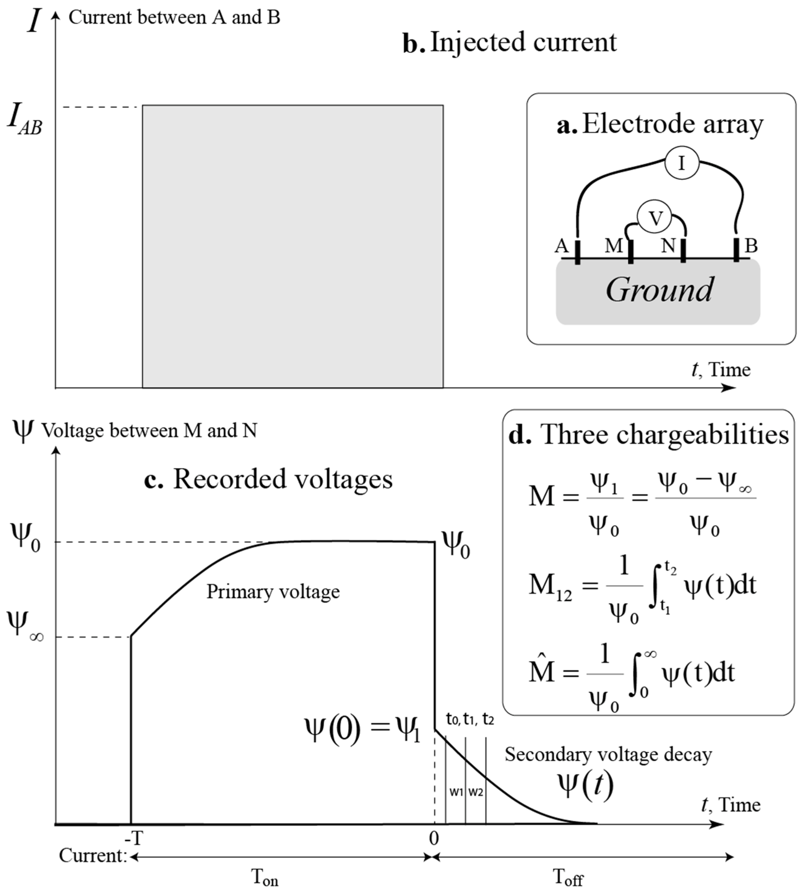
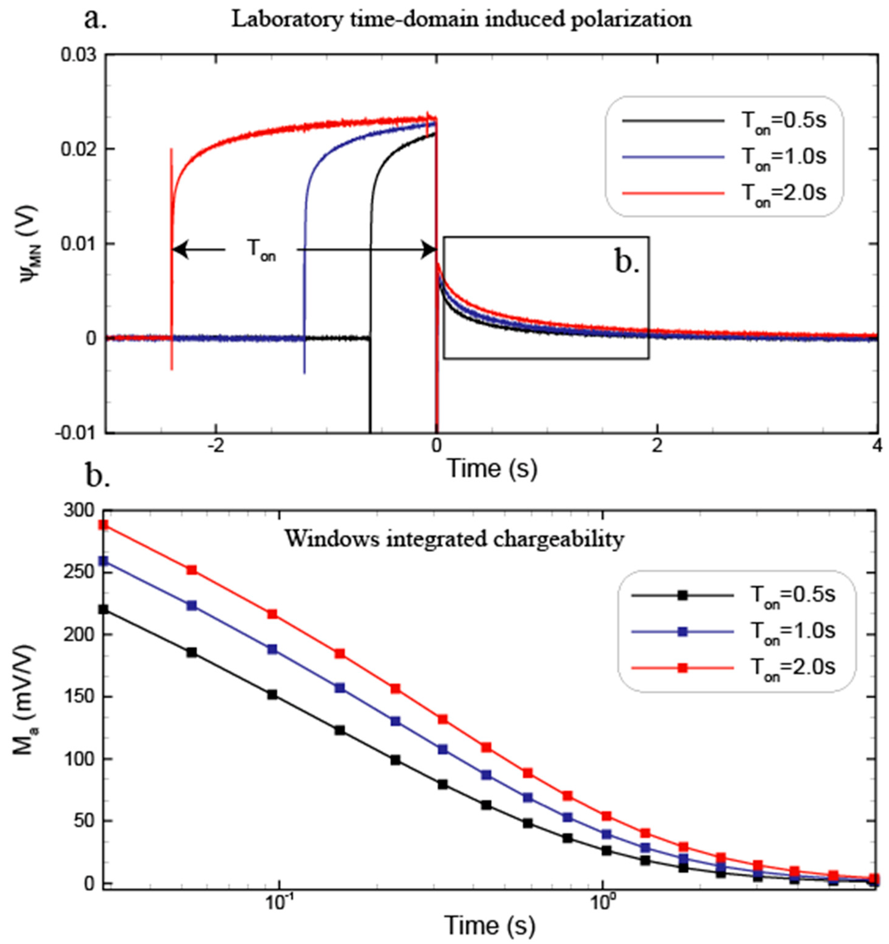
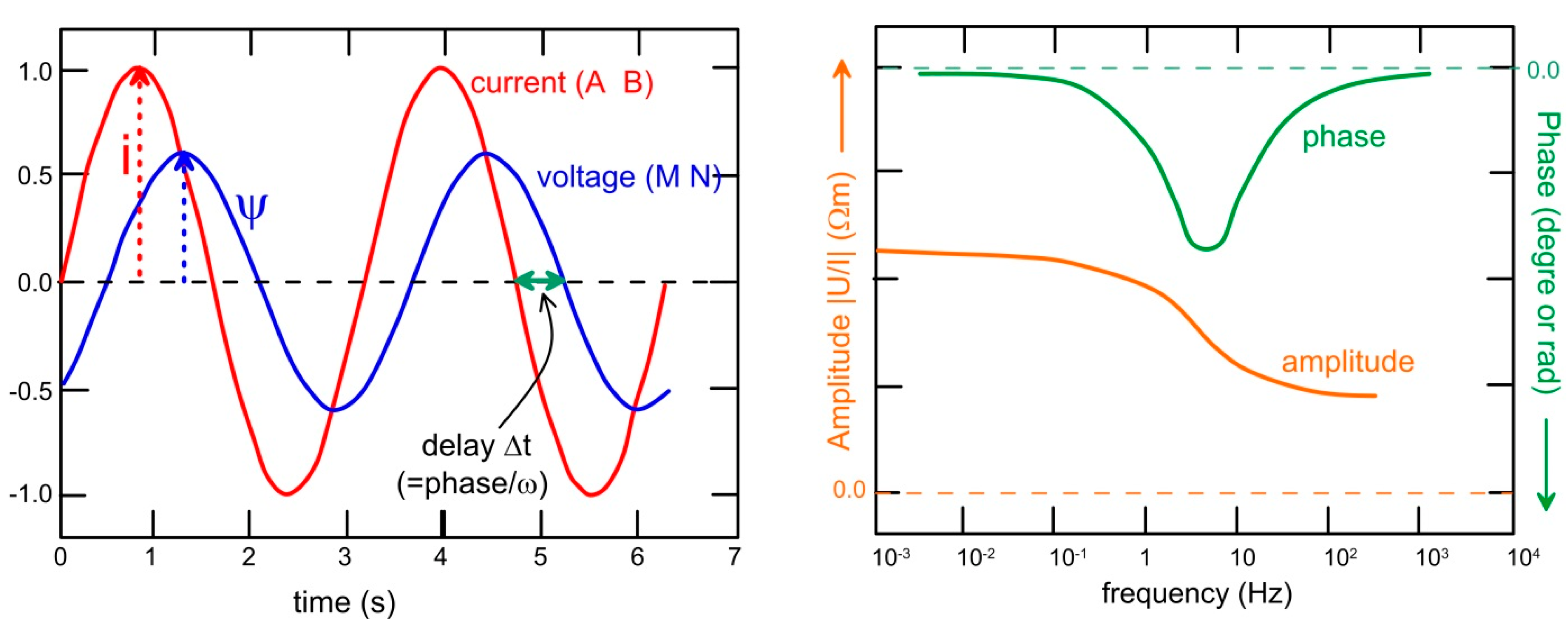
2. Time-Domain and Frequency-Domain Induced Polarization

Induced polarization was first described in the seminal book of Conrad Schlumberger (1920) [2]. It refers to the reversible storage of electrical charges in the ground under the application of a primary (low-frequency) electrical field or electrical current. This reversible storage of electrical charges occurs at some polarization length scales of the porous medium that correspond to the grain and pore scales [37,39,40,48]. In turn, this reversible storage of electrical charges is responsible for a secondary electrical current or electrical field that is associated with the electro-diffusion of the accumulated charge carriers through the gradients in the electrochemical potential of the charge carriers. The secondary electrical field or current is therefore “induced” by the primary current or electrical field. With that being said, the term “induction” is usually avoided because it refers to another specific mechanism in electromagnetic studies.

This secondary electrical field can be remotely measured by using a network of electrodes. The relationship between the output (measured) secondary electrical field and the applied signal (e.g., the primary current or electrical field) can be linear or nonlinear. In this paper, we consider that the Earth is a time-invariant linear filter and that it can therefore be analyzed by using linear time-invariant system theory. Such an approach reveals the transfer function of porous media (with or without metallic minerals) in the frequency domain and their impulse responses in the time domain [49]. Causality is a necessary constraint on the transfer function of the Earth for induced polarization. As an example, an RC circuit (R denotes the resistance and C the capacitance) falls into this category. For nonlinear induced-polarization effects, the interested readers are directed to specific publications, such as Hall and Olhoeft (1986) [49] and Chu and Bazant (2006) [50]. With that being said, the nonlinear polarization mechanisms have not been explored very much in geophysics.

The procedure that is used to measure induced polarization in the laboratory or in the field is similar to one of the classical electrical methods [2]. An electrical current is injected into the ground or through a core sample through a bipole of (current) electrodes (A and B). We observe the associated voltage or electrical potential difference at a pair of receiving (voltage) electrodes (M and N). Figure 1 and Figure 2 illustrate the concept of time-domain induced polarization and chargeability. The existence of various definitions of the chargeability makes the literature, at first, a bit cryptic to read for newbies in the field. Usually, the measurements are performed in the time domain in the field, or in the frequency domain in the laboratory (Figure 3, see [51]). With that being said, it is worth noticing that more and more field investigations are based on frequency-domain induced polarization measurements [28,52,53,54,55]. In our viewpoint, it does not really matter if the measurements are performed in the time domain or the frequency domain. The date can even be acquired in the time domain and can be inverted in the frequency domain, or vice versa.

In time-domain induced polarization, the process of polarization is characterized by a chargeability, while, in the frequency domain, the induced polarization is characterized by complex conductivity spectra and a phase. The phase and the chargeability can be related to each other in a manner that is similar to the normalized chargeability (product of the chargeability by the conductivity) and the quadrature conductivity (the phase times and the conductivity also correspond to the imaginary part of the complex conductivity (e.g., van Voorhis et al., 1973 [56]; Revil et al., 2017b [57]), in the context of the constant phase model). The transfer function corresponds to the filter that is associated with the ground (or with a core sample). As far as induced polarization is concerned, the most famous empirical or parametric “filters” are known as the Debye, the Cole–Cole, or the constant-phase model transfer functions [58]. We will come back to some of these filters in the present paper.

3. Model in Absence of Background Polarization

3.1. Implication of the Maxwell–Clausius–Mossotti Equation

We consider a mixture of metallic grains in a background, such as is shown in Figure 4. The grains are considered to be spheres, and the material is assumed to be isotropic at all scales. The metallic grains and the clay particles polarize with distinct polarization mechanisms and polarization levels (Figure 5; see Marshall and Madden 1959 [5] for a discussion on this topic). The typical spectra for such mixtures (e.g., pyrite or slag with sand) are shown in Figure 6 and Figure 7.

We first consider that the background material (in which the metallic particles are embedded) is a pure conductor and does not polarize. This assumption will be relaxed later on. We write the conductivity of the background as ${\sigma }_b$ (pure real number) instead of ${\sigma }_b*$ (Figure 4). The quantity ${\sigma }_b$ depends on the porosity, the cation exchange capacity, and the pore water conductivity; an expression of the conductivity of the background material will be provided later (see Section 4.2 below and Winsauer and McCardell, 1953 [59]; Waxman and Smits, 1968 [60]; Vinegar and Waxman, 1984 [61]). We start here with the well-established form of the Maxwell–Clausius–Mossotti equation [37,62,63] to analyze the complex conductivity of the mixture ($\sigma *$):

$$\frac{\sigma *-{\sigma }_b}{\sigma *+2{\sigma }_b}={\phi }_m\left(\frac{{\sigma }_m*-{\sigma }_b}{{\sigma }_m*+2{\sigma }_b}\right)$$

(1)

where $\sigma *$ denotes the complex conductivity of the mixture (background with metallic particles); ${\phi }_m$ denotes the volume fraction of the metallic particle; and ${\sigma }_m*$ is the complex conductivity of the metallic particles [46,64]. The in-phase and the quadrature conductivities of the composite material correspond to the real and imaginary parts of $\sigma *$ (i.e., $\sigma \prime \equiv \mathrm{Re}(\sigma *)$ and $\sigma ″\equiv \mathrm{Im}(\sigma *)$). Equation (1) is only valid for small concentrations of metallic particles (typically, ${\phi }_m\le 0.16$ (e.g., Wong, 1979 [37]), but we will see that, actually, the model developed below works up to ${\phi }_m\sim 0.22$).

In Equation (1), the quantity $f(i\omega )=\left({\sigma }_m*-{\sigma }_b\right)/\left({\sigma }_m*+2{\sigma }_b\right)$ denotes the (complex-valued) “reflection coefficient” [62], which is connected to the dipole moment of the metallic grains. If the conductivity of the metallic particles is very large with respect to the background ($\left|{\sigma }_m*\right|>>{\sigma }_b$), we have $f(i\omega )$ = 1. For insulating particles ($\left|{\sigma }_m*\right|=0$), we obtain $f(i\omega )$ = −1/2.

In semiconductors such as pyrite and magnetite, the charge carriers inside the metallic particle are electrons and positive holes (Figure 5 and Figure 8). At low frequencies and in the absence of redox active species in the pore water, these carriers are blocked by the surface of the metallic grain (Figure 5). This blocking effect (perfect capacitance) is responsible for the accumulation of the charge carriers at the boundary of the metallic particle in the applied electrical field. In our approach, this intraparticle mechanism is responsible for the observed polarization. The case where these charge carriers can be exchanged with the surrounding electrolyte (leaky capacitance) will not be discussed in the present paper (see [37]).

If the applied (external) electrical field is removed, the n- and p-charge carriers will go back to their statistical equilibrium positions through electro-diffusion (the driving force for the motion is an electrochemical potential, see Section 3.2 below). We can conclude that the metallic grains would appear as insulators at low frequencies. Therefore, we have $f(i\omega )$ = −1/2 at low-frequencies (i.e., for the direct current (DC) condition). Indeed, once a grain is fully polarized, all of its charge carriers are frozen as long as the electrical field remains constant. In some sense, we can say that polarization is detrimental to conduction. At high frequencies, the conductivity of the metallic grain is pretty large (much greater than the background material [66]). Therefore, at high frequencies, $f(i\omega )$ = 1.

The transition between the low-frequency and high-frequency domains is controlled by a relaxation time. From a dimensional analysis, this relaxation time depends on the radius of the grains and on the diffusion coefficient of the charge carriers in the metallic particles. If the grains have different sizes, this transition is controlled by a (probability) distribution of the relaxation times that can be related to a (probability) distribution of the polarization length scales [67]. Finding an expression of the relaxation time is therefore a key objective of any model of the polarization of porous media.

Equation (1) provides an explicit expression of the complex conductivity of the mixture:

$$\sigma *={\sigma }_b\left(\frac{1+2{\phi }_{m}f(i\omega )}{1-{\phi }_{m}f(i\omega )}\right)$$

(2)

For small concentrations of metallic particles, we can approximate Equation (3) by:

$$\sigma *={\sigma }_b\left[1+3{\phi }_{m}f(i\omega )+\dots \right]$$

(3)

by using a first-order Taylor development in ${\phi }_m$.

If the grain-size distribution of the metallic particles is close to a log-normal distribution, the Cole–Cole model is known to provide an accurate representation of the induced polarization spectra of the disseminated ores [35]. Figure 6 and Figure 7 are examples of spectra that could be fitted with a Cole–Cole model [35]. We therefore write the complex conductivity of the mixture by using a Cole–Cole model as [46]:

$$\sigma *={\sigma }_{\infty }+\frac{{\sigma }_0-{\sigma }_{\infty }}{1+{(i\omega {\tau }_0)}^c}$$

(4)

$$\sigma *={\sigma }_{\infty }\left(1-\frac{M}{1+{\left(i\omega {\tau }_0\right)}^c}\right)$$

(5)

$$M=\frac{{\sigma }_{\infty }-{\sigma }_0}{{\sigma }_{\infty }}=\frac{{\rho }_0-{\rho }_{\infty }}{{\rho }_0}$$

(6)

where M denotes the (total) chargeability of the material; ${\rho }_0=1/{\sigma }_0$ (DC resistivity) and ${\rho }_{\infty }=1/{\sigma }_{\infty }$ (the M is called the “polarizability” in the Russian literature); and where ${\tau }_0$ denotes the relaxation time that is associated with the depolarization of a fully polarized grain. The chargeability describes the ratio of the polarization to the conduction. Hereinafter, we will also use the normalized chargeability (i.e., the product of the chargeability by the electrical conductivity (M_n = M ${\sigma }_{\infty }$ = ${\sigma }_{\infty }-{\sigma }_0$), which better characterizes the polarization process alone). Our goal is to now provide a physical meaning for the parameters that are involved in Equation (5) or Equation (6) (i.e., M, ${\sigma }_{\infty }$, c, and ${\tau }_0$). The exponent c, which is called the Cole–Cole exponent, can be related to the broadness of the relaxation-time distribution [34,68,69].

With the Cole–Cole model, the reflection coefficient is given by $f(i\omega )=1-(3/2)/[1+{(i\omega {\tau }_0)}^c]$. This can be compared with models on the basis of the polarization of the diffuse layer (see Bücker et al., 2018a [39], their Appendix C; and Wong, 1979 [37]): $f(i\omega )\approx 1-(3/2)/[1+i\omega {\tau }_1]$(diffuse layer polarization) with ${\tau }_1=a{\lambda }_D/2D_{(\pm )}$ and $f(i\omega )\approx 1-(3/2)/[1+{(i\omega {\tau }_2)}^{1/2}]$ (volume-diffusion relaxation), with ${\tau }_2=a^2/4D_{(\pm )}$, where $D_{(\pm )}$ is the diffusion coefficient of the ions in the pore water (assuming a binary symmetric of 1:1 electrolyte with the same diffusion coefficient for the cations and anions: ~10⁻⁹ m² s⁻¹); and ${\lambda }_D$ is the Debye length (in m) that is associated with the thickness of the diffuse layer around the grain.

Our goal now is to determine an expression of the relaxation time (${\tau }_0$). From the dimensional analysis, the main relaxation time (for the complex conductivity, Equation (5)) is written as: ${\tau }_0=a^2/D_a$ [70], where $D_a$ is the (apparent) diffusion coefficient of the charge carriers that are responsible for the polarization of the conductive particles. In Equation (5), ${\sigma }_0$ and ${\sigma }_{\infty }$ denote, respectively, the DC conductivity ($\omega <<1/{\tau }_0$) and the high-frequency conductivity of the porous material ($\omega >>1/{\tau }_0$). Olhoeft (1985) [6] determined that the relationship between the relaxation time of the pyrite-bearing porous media and the radius (a) of the metallic particles is ${\tau }_0\approx 3\times {10}^5{a}^2$, and that, therefore, using ${\tau }_0=a^2/D_a$ leads to $D_a$ = 3.0 × 10⁻⁵ m² s⁻¹.

Tarasov and Titov (2013) [69] show that the Cole–Cole relaxation time (${\tau }_0$) is related to the time constant that corresponds to the peak of the phase ($\tau$) by ${\tau }_0=\tau {\left(1-M\right)}^{1/2c}<\tau$. If a Cole–Cole model is used for the resistivity (see, for instance, the Cole–Cole resistivity model that is used in [11]), the relaxation time in the resistivity is given by ${\tau }_{\rho }={\tau }_0{\left(1-M\right)}^{-1/c}>{\tau }_0$ [18]. Note that, for small chargeabilities, ${\tau }_{\rho }\approx {\tau }_0\left(1+M/c+\dots \right)$, and, therefore, this time constant increases linearly with the chargeability for materials that are characterized by the same radius for the metallic particles [11]. An explicit derivation of the relaxation time is found below in Section 3.2.

We are now going to provide an explicit formula for this chargeability [46,64]. At a very high frequency ($f(i\omega )\to 1$), the metallic particles appear infinitively conductive [37] since the mobility of the charge carriers in the metallic particles is high and the electromigration of the charge carriers is not limited by the boundary of the metallic particle. To the contrary, at a very low frequency ($f(i\omega )\to -1/2$), the metallic particles appear insulating [37]. Indeed, at very low frequencies, all of the available charge carriers have reached the boundary of the metallic grain. The grain is fully polarized, and all of these charges are lost for the conduction process. From these considerations and by using Equation (4), we obtain:

$${\sigma }_{\infty }={\sigma }_b(1+3{\phi }_m)$$

(7)

$${\sigma }_0={\sigma }_b\left(1-\frac{3}{2}{\phi }_m\right)$$

(8)

Equations (8) and (9) can also be derived by using the differential effective medium theory, as is further discussed below. From Equations (7)–(9), the chargeability is approximately given by:

$$M\approx \frac{9}{2}{\phi }_m$$

(9)

If we start directly with the complete Maxwell–Clausius–Mossotti equation, without any approximation, we obtain (after few algebraic manipulations) the following (more general) expression for the chargeability for spherical metallic particles immersed in a conductive background [37,71]:

$$M=\frac{9{\phi }_m}{2+5{\phi }_m+2{\phi }_m{}^2}$$

(10)

Since $M\le 1$, Equation (10) is strictly valid only for ${\phi }_m\le 2/9\approx 0.22$ (22% vol. content of the mixture).

3.2. The Relaxation Time

The spectral induced polarization measurements from the literature have demonstrated the existence of a relationship between the relaxation time (${\tau }_0$) and the diameter of the metallic grains (a) [11,41,46,64,70,72]. In order to go one step further in the understanding of the relaxation time (or the distribution of the relaxation times), numerical simulations can be performed to gain a good physical understanding of the underlying physics [41,43]. The local equations to solve correspond to the Poisson–Nernst–Planck equations that describe both the diffusion and the electromigration of the charge carriers [5,73], and both inside and outside of the metallic particles. We consider the case of a metallic particle that is immersed in a background of 1:1 electrolyte (e.g., NaCl, KCl). In the metallic particle, the charge carriers are holes and electrons (Figure 8), and in the pore fluid, the charge carriers are anions and cations.

We consider an applied harmonic electrical field (${\mathsf{E}}_a={\mathsf{E}}_0\exp \left(i\omega t\right)$) with ${\mathsf{E}}_0$ as the amplitude. The concentrations and the electrical potential are given by the sum of the values at equilibrium plus perturbations [39,40]:

$$C_{(\pm )}^{}(\mathit{r},t)=C_{(\pm )}^0+\delta C_{(\pm )}^{}(\mathit{r},t)e^{i\omega t}$$

(11)

$${\psi }_e(\mathit{r},t)=\delta {\psi }_e(\mathit{r},t)e^{i\omega t}$$

(12)

$$C_{(+)}^0=C_{(-)}^0$$

(13)

where ${\psi }_e$ (V) describes the electrical potential that is external to the metallic particle; $C_{(\pm )}^0$ (m⁻³) describe the equilibrium concentrations of the ions in the electrolyte in the absence of an external applied field; and $\delta C_{(\pm )}^{}$ and $\delta {\psi }_e$ represent the perturbations of the concentration and the potential around the equilibrium, respectively. In the electrolyte, the driving force that controls the movement of the ionic charge carriers is the gradient in their electrochemical potential:

$$\nabla {\tilde{\mu }}_{(\pm )}^{}=-(\pm e)\mathsf{E}+k_{b}T\nabla \ln C_{(\pm )}^{}$$

(14)

where e = 1.6 × 10⁻¹⁹ C (elementary charge); k_b = 1.381 × 10⁻²³ m² kg s⁻² K⁻¹ (Boltzmann constant); and T is the absolute temperature (in K). The mobilities and diffusion coefficients are related to each other by the Nernst–Einstein relationship:

$${\beta }_{(\pm )}=\left|q_{(\pm )}\right|b_{(\pm )}=\frac{\left|q_{(\pm )}\right|D_{(\pm )}}{k_{b}T}$$

(15)

where $q_{(\pm )}=\pm e$ denotes the charge of the cations and anions. The diffusion flux densities are given by the Nernst–Planck equations [74,75,76]:

$${\mathsf{J}}_{(\pm )}^{}=-b_{(\pm )}^{}{C}_{(\pm )}^{}\nabla {\tilde{\mu }}_{(\pm )}^{}$$

(16)

$${\mathsf{J}}_{(\pm )}^{}=\left[(\pm e)\frac{D_{(\pm )}^{}{C}_{(\pm )}^0}{k_{b}T}\nabla \delta {\psi }_e(\mathit{r},t)-D_{(\pm )}^{}\nabla \delta C_{(\pm )}^{}(\mathit{r},t)\right]e^{i\omega t}$$

(17)

The continuity equation for the ionic species can be expressed as [37]:

$$\nabla \cdot {\mathsf{J}}_{(\pm )}^{}=-\frac{\partial C_{(\pm )}^{}(\mathit{r},t)}{\partial t}$$

(18)

Combining Equations (18) and (19) yields the following partial differential equation:

$$(\pm e)\frac{D_{(\pm )}^{}{C}_{(\pm )}^0}{k_{b}T}{\nabla }^2\delta {\psi }_e(\mathit{r},t)-D_{(\pm )}^{}{\nabla }^2\delta C_{(\pm )}^{}(\mathit{r},t)=-i\omega \delta C_{(\pm )}^{}(\mathit{r},t)$$

(19)

The electrical potential and the ionic concentrations are also related to each other by Gauss’s law [77]:

$${\epsilon }_f\nabla \cdot \mathsf{E}=\rho$$

(20)

where $\rho$ (C m⁻³) denotes the charge density, which is defined as:

$$\rho =e\left[C_{(+)}^{}(\mathit{r},t)-C_{(-)}^{}(\mathit{r},t)\right]$$

(21)

Combining Equations (12), (13), (21), and (22) yields:

$${\nabla }^2\delta {\psi }_e(\mathit{r},t)=-\frac{Ne}{{\epsilon }_f}\left[\delta C_{(+)}^{}(\mathit{r},t)-\delta C_{(-)}^{}(\mathit{r},t)\right]$$

(22)

where N denotes the Avogadro number (6.02 × 10²³ mol⁻¹). The same type of equations can be written inside of the metallic particle for the two charge carriers: the electrons and the p-hole (especially for semiconductors), which also obeys the same partial differential equation that is derived from the Poisson–Nernst–Planck equations, the continuity equations, and Gauss’s law [78,79]:

$$(\pm e)\frac{D_{(\pm )}^m{C}_{(\pm )}^m}{k_{b}T}{\nabla }^2\delta {\psi }_i(\mathit{r},t)-D_{(\pm )}^m{\nabla }^2\delta C_{(\pm )}^m(\mathit{r},t)=-i\omega \delta C_{(\pm )}^m(\mathit{r},t)$$

(23)

$${\nabla }^2\delta {\psi }_i(\mathit{r},t)=-\frac{Ne}{{\epsilon }_S}\left[\delta C_{(+)}^m(\mathit{r},t)-\delta C_{(-)}^m(\mathit{r},t)\right]$$

(24)

In these equations, $D_{(\pm )}^m$ denote the diffusion coefficients of the positive charge carriers (p-holes) and the negative charge carriers (electrons) in the semiconductor; ${\epsilon }_S$ denotes the dielectric constant of the solid metallic grain; and $\delta {\psi }_i$ denotes the perturbed potential inside the metallic particle.

For the numerical simulations, we consider a pyrite grain (FeS₂; grain size is 2 μm; electrons and p-holes) that is immersed in a background electrolyte with KCl (${\mathrm{K}}^{+}$ and ${\mathrm{Cl}}^{-}$), with ${\sigma }_S^{\infty }$(pyrite) = 1000 S m⁻¹, ${\mathrm{D}}_{\mathrm{e}-}={\mathrm{D}}_{\mathrm{hole}}$ = 2.9 × 10⁻⁵ m² s⁻¹, ${\mathrm{D}}_{{\mathrm{K}}^{+}}={\mathrm{D}}_{{\mathrm{Cl}}^{-}}$ = 1.7 × 10⁻⁹ m² s⁻¹, and the relative dielectric constant for the background is 80, the relative dielectric constant for the solid grains (pyrite) is 10.9, and with a temperature of 293 K (20 °C), and various salinities in the range from 10⁻³ to 0.5 Mol m⁻³. The partial differential equations are solved in time by using a finite difference approximation that is based on Euler’s method, whereas the spatial discretization is performed by using the finite element method (FEM) (see [41,43] for details).

The applied boundary conditions that were used in the numerical simulations are as follows (Figure 9): (1) The Dirichlet boundary condition to the right and left sides of the domain (a constant current source); (2) The Neumann condition at the top and the bottom of the model (where we assume that no flux in the charges is allowed (the normal derivative of the potential is null). This corresponds to the insulation of the boundary conditions at these frontiers; (3) The blocking boundary condition, which was also imposed on the electrolyte/grain interface ($\partial {\mathrm{J}}_{(\pm )}/\partial \widehat{n}=0$ (where $\widehat{n}$ is the unit vector on the surface of the grains)), and therefore we neglect here the redox processes that would be responsible for the leaking capacitance that is associated with the grain. The charge concentration and the charge mobility in each region (grain and electrolyte) are defined by using a space function, the ions are defined in the electrolyte, whereas the electrons and holes are defined in the metallic grain; (4) The initial condition (for a time-dependant problem); before the current injection (at t < 0), we imposed the following conditions: ψ = 0 everywhere in the medium; $c_{cation}=c_{anion}$ and homogenous in the solution; and $c_{electron}=c_{hole}$ and homogenous in the grain. The mesh that was used for the 2D simulations is shown in Figure 9.

Figure 10 shows a 2D map of the potential distribution that resulted from the solution of the Poisson–Nernst–Planck equations at two different times (left): directly after the beginning of the injection (0.03 µs), and (right) after 1.5 µs of the current injection. The particle is in the center of the model, and so the grain is obtaining constant potential after a few nanoseconds of the current injection. During the current injection, the charge accumulates at the interface grain/electrolyte until a critical equilibrium state is reached (1.5 µs). This forms a charge condensation at the interface between the metallic grain and the background electrolyte, which forms a dipole at the scale of the grain.

When the current is stopped, the accumulated charges relax to their initial (equilibrium) positions, both outside and inside the metallic particle, which generates a secondary potential decaying in time. Figure 10 shows maps of the secondary potential distribution and its fluctuations over time. By using such numerical simulations, Abdulsamad et al. (2020) [43] were able to reproduce the dependence of the relaxation time on the background conductivity, which was controlled here by the salinity (Figure 11 and Figure 12). The vertical shift between the time relaxation that resulted from the simulation and that which resulted from the measurements was caused by the difference in the grain sizes. The observed dependence of the relaxation time on the salinity could be explained by considering the metallic grain as an electrical dipole that is formed during the current injection. This electrical dipole impacts the electric potential and, consequently, the charge distribution in its vicinity. Figure 10 shows the variation in the charge concentration away from the metallic particle/electrolyte interface at the end of the current injection time. We notice that, as long as the electrolyte concentration is low, the influence of the electric dipole is farther from the grain/electrolyte interface, which provides a higher relaxation time (larger distance for ions to go back to the equilibrium state). These results are consistent with the model that was discussed in the previous sections.

For small grains (<100 μm), the induced-polarization response is dominated by field-induced diffuse layers outside of the metallic grains, and the model that was developed by Bücker et al. (2018a,b) [39,40] can be used to understand the process, as discussed above. For large grains (>500 μm at low salinity), we can neglect the formation of field-induced diffuse layers outside of the grains. For a grain with a radius of 1.5 cm, the relaxation time is in the order of a few seconds. The numerical simulations show that the relaxation time decreases with the increase in the conductivity of the background electrolyte, and that it increases with the increase in the metallic particle conductivity itself (Figure 12). This dependence is written as:

$${\tau }_0=\frac{a^2}{D_m}\left(1+\frac{{\sigma }_S^{\infty }}{{\sigma }_b}\right)\approx a^2\frac{{\sigma }_S^{\infty }}{D_m{\sigma }_b}$$

(25)

where ${\sigma }_S^{\infty }$ denotes the instantaneous conductivity of the metallic grain, and ${\sigma }_b$ denotes the background conductivity. Thus, the apparent diffusion coefficient is given by $D_a=D_m{\sigma }_b/{\sigma }_S^{\infty }$. Since the conductivity of the grains depends on the diffusion coefficient of the charge carriers ($D_m$), this means that the $D_a$ is independent of the diffusion coefficient of the charge carriers in the metallic particle; however, it depends on the concentration of the charge carriers in these metallic particles [66,80]. This is perhaps a paradox of the proposed polarization process.

The model that is developed in Section 3.1 above shows a linear relationship between the chargeability and the volume fraction of the metallic particles in the medium [41,43,46,64,70]. From the numerical simulations, and by using the potential difference that is picked up between two points (M and N) (Figure 9), the chargeability (M) is calculated as the ratio between the secondary voltage (in V), which is measured just after stopping the current, and the primary voltage (in V), which is measured at the end of the current injection [81]. We will come back to this relationship below in Section 6.3. Figure 12b shows the results of the numerical simulations for the chargeability versus the volume of the metallic particles in the medium. The linear relationship that is evidenced by the numerical simulations is consistent with both the theory and the experimental data (see Figure 13).

4. Model in Presence of Background Polarization

4.1. Background Polarization and Chargeability

Our goal in this section is to explore the effect of the chargeability of the background on the overall chargeability of the material. For this purpose, a slightly more general approach than the Maxwell–Clausius–Mossotti equation is preferred, such as the solution of the differential effective medium (DEM) theory [83]. For metallic particles that are suspended in a polarizable background (Figure 4), we have below the iso-conductivity point [83,84]:

$$\sigma *={\sigma }_b*{(1-{\phi }_m)}^{\frac{m_m}{1-m_m}}{\left(\frac{{\sigma }_m*-{\sigma }_b*}{{\sigma }_m*-\sigma *}\right)}^{\frac{m_m}{1-m_m}}$$

(26)

where ${\sigma }_b*$ denotes the complex conductivity of the background rock, and $m_m$ (dimensionless) denotes a grain-shape exponent of the metallic particles [83]. If the metallic particles are much more conductive with respect to the background material (and the conductivity of the mixture), Equation (27) reduces to:

$$\underset{\left|{\sigma }_m*\right|>>\left|{\sigma }_b*\right|}{\lim }\sigma *\approx {\sigma }_b*{(1-{\phi }_m)}^{\frac{m_m}{1-m_m}}$$

(27)

If the number of the metallic particles is small (in the case of a dilute suspension of metallic particles that are immersed in a background material), we have:

$$\underset{\left|{\sigma }_m*\right|>>\left|{\sigma }_b*\right|}{\lim }\sigma *\approx {\sigma }_b*\left(1+\frac{m_m}{m_m-1}{\phi }_m+\dots \right)$$

(28)

This case corresponds to the high-frequency limit that is discussed above in Section 3, for which we obtain an expression of the instantaneous conductivity of the mixture:

$${\sigma }_{\infty }\approx {\sigma }_b^{\infty }\left(1+\frac{m_m}{m_m-1}{\phi }_m+\dots \right)$$

(29)

In this case, there is an increase in the instantaneous conductivity with the volumetric concentration of metallic particles. The second case corresponds to the case that the metallic particles appear insulating (i.e., at low frequencies). In this case, all of the charge carriers of the metallic particle have accumulated and they do not contribute anymore to the conductivity of the metallic particle. We have:

$$\sigma *={\sigma }_b*{(1-{\phi }_m)}^{m_m}{\left(\frac{1-{\sigma }_m*/{\sigma }_b*}{1-{\sigma }_m*/\sigma *}\right)}^{m_m}$$

(30)

$$\sigma *\approx {\sigma }_b*(1-m_m{\phi }_m+\dots )$$

(31)

where Equation (32) is obtained from Equation (31) by using a first-order Taylor expansion in ${\phi }_m$. In this case, there is a decrease in the DC conductivity with the volumetric concentration of metallic particles. Equation (32) can be used to determine the low-frequency (DC) limit of the complex conductivity:

$${\sigma }_0\approx {\sigma }_b^0(1-m_m{\phi }_m+\dots )$$

(32)

By using Equations (30) and (33) and the definition of the chargeability (see Equation (7)) yields, after a few algebraic manipulations, we obtain the following expression for the chargeability:

$$M\approx 1-\frac{{\sigma }_b^0}{{\sigma }_b^{\infty }}\left[1-\left(\frac{m_m{}^2}{m_m-1}\right){\phi }_m\right]$$

(33)

Two extreme situations can be discussed. First, in the absence of metallic particles, the chargeability is given by the chargeability of the background ($M_b$); indeed:

$$\underset{{\phi }_m=0}{\lim }M=1-\frac{{\sigma }_b^0}{{\sigma }_b^{\infty }}=M_b$$

(34)

The second case is the case of spherical ($m_m$ = 3/2) metallic grains in a nonpolarizable background. We have:

$$\underset{M_b=0}{\lim }M=\left(\frac{m_m{}^2}{m_m-1}\right){\phi }_m=\frac{9}{2}{\phi }_m=M_m$$

(35)

where $M_m$ is the chargeability that is associated with the metallic particles only (see Section 3 above, Equations (10) and (11)). From Equations (34)–(36), the chargeability of the material is given by:

$$M=1-(1-M_b)(1-M_m)$$

(36)

An expression of the background chargeability will be given below in Equation (48). For small background and metallic chargeabilities $(M_b,M_m)<<1$, Equation (37) simplifies to [46,64]:

$$M\approx M_b+M_m$$

(37)

In other words, the chargeabilities are cumulative as long as they are small. Equations (37) and (38) are very important equations for understanding the chargeability of complex porous media with various sources of polarization. We now need to generalize the Cole–Cole model for such media. This is performed in the next section.

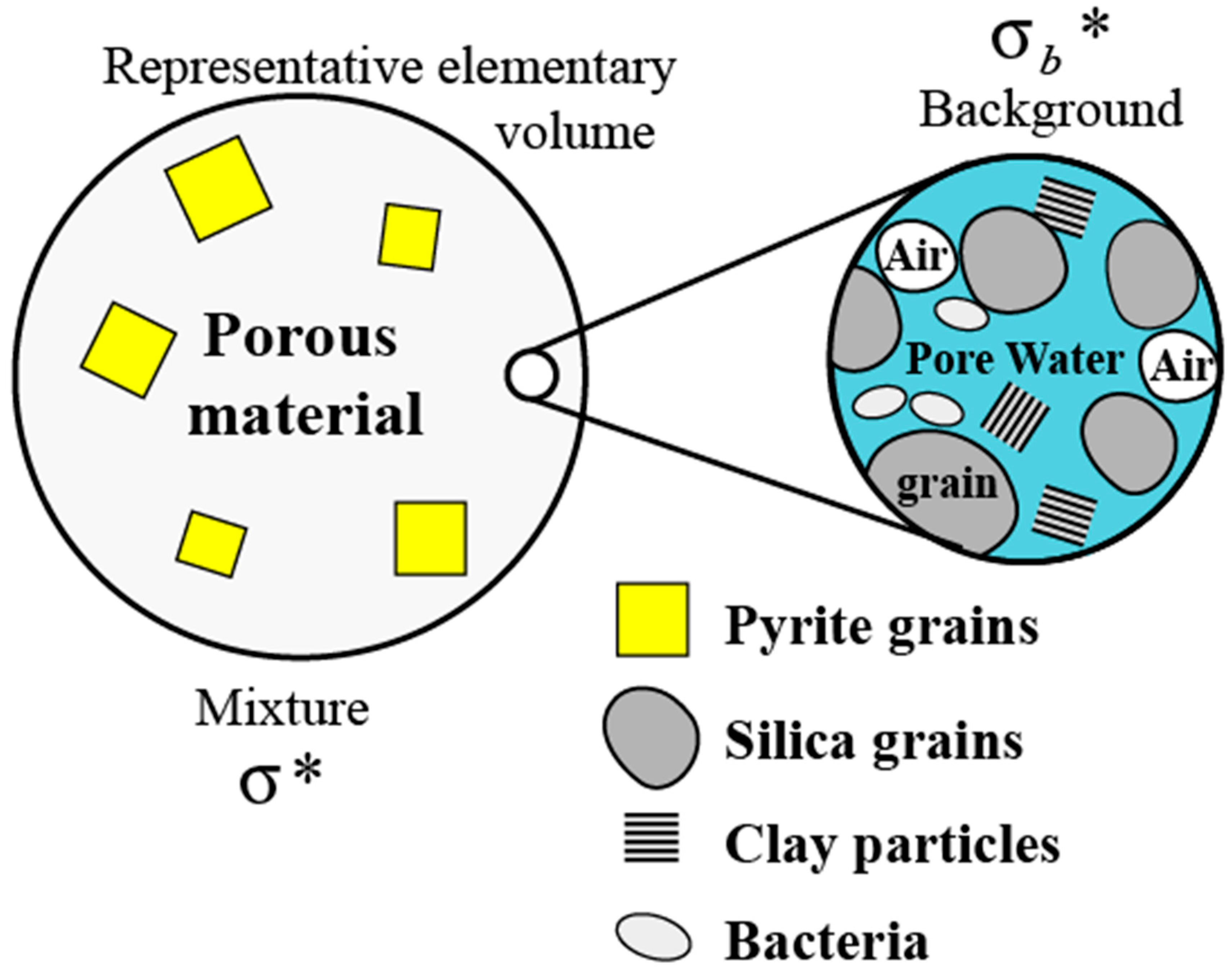
4.2. A Generalized Mixture Model

We assume, in this section, a porous material with K-polarization processes, and each of them is described by a Cole–Cole transfer function. Generally speaking, this could be the polarization of the nonmetallic grains, the polarization of the metallic grains, and even the polarization of bacteria in the pore space for mining wastes, for instance (Figure 4). A generalization of the complex conductivity of the Cole–Cole model for K-induced polarization distributions can be written as:

$$\sigma *={\sigma }_{\infty }\left(1-{\displaystyle \sum _{k=1}^K\frac{M_k}{1+{(i\omega {\tau }_k)}^{c_k}}}\right)$$

(38)

$$M_k=\frac{{\sigma }_k^{\infty }-{\sigma }_k^0}{{\sigma }_k^{\infty }}$$

(39)

$${\sigma }_0={\sigma }_{\infty }\left(1-{\displaystyle \sum _{k=1}^K{M}_k}\right)$$

(40)

where $M_k$, $c_k$, and ${\tau }_k$ denote the chargeability, the Cole–Cole exponent, and the relaxation time for the process (k) for a total number of K polarization processes, respectively. In the case of mineralized rocks, we consider two polarization mechanisms, as discussed in the previous sections. For two polarization processes (metallic and non-metallic grains), we have:

$$\sigma *={\sigma }_{\infty }\left(1-\frac{M_1}{1+{(i\omega {\tau }_1)}^{c_1}}-\frac{M_2}{1+{(i\omega {\tau }_2)}^{c_2}}\right)$$

(41)

$${\sigma }_{\infty }={\sigma }_1^{\infty }+{\sigma }_2^{\infty }$$

(42)

$${\sigma }_0={\sigma }_{\infty }\left(1-M_1-M_2\right)$$

(43)

where M₁ and M₂ are the chargeabilities (dimensionless), c₁ and c₂ are the two Cole–Cole exponents (dimensionless), and τ₁ and τ₂ are the relaxation times (expressed in s). Indexes 1 and 2 refer to two dispersion processes, respectively (metallic and nonmetallic grains). With these relationships, we have, ${\sigma }_0\ne {\sigma }_1^0+{\sigma }_2^0$ and ${\sigma }_1^{\infty }\ne {\sigma }_2^0$. If the total chargeability is defined by $M=({\sigma }_{\infty }-{\sigma }_0)/{\sigma }_{\infty }$, we have:

$$M=M_1+M_2$$

(44)

and since $0\le M\le 1$, we have $0\le M_1+M_2\le 1$. In our model, one of the two mechanisms of polarization (for instance, Mechanism 1) corresponds to the polarization of metallic particles, while the second mechanism (therefore, Mechanism 2) corresponds to the polarization of the electrical double layer of the insulating grains that form the skeleton of the background material (Figure 5).

By using a volume-averaging approach, Revil (2013) [85] obtained the following expressions for the high- and low-frequency conductivities of the background material:

$${\sigma }_2^{\infty }=\frac{1}{F}{\sigma }_w+\left(\frac{1}{F\varphi }\right){\rho }_{g}B\hspace{0.17em}\mathrm{CEC}$$

(45)

$${\sigma }_2^0=\frac{1}{F}{\sigma }_w+\left(\frac{1}{F\varphi }\right){\rho }_g(B-\lambda )\mathrm{CEC}$$

(46)

Equation (46) can be used for the conductivity of the background material in Section 3. In these equations, ${\sigma }_w$ (in S m⁻¹) denotes the pore water conductivity (which depends on both salinity and temperature); F (dimensionless) is the intrinsic formation factor that is related to the connected porosity (ϕ) (dimensionless) by the first Archie’s law (F = ϕ^−m, where m (dimensionless) is called the “first Archie exponent” or the “porosity exponent” [86]); m is the cementation exponent (the porosity exponent or first Archie’s exponent) that is associated with the grain shape of the nonmetallic grains; ${\rho }_g$ is the grain density (in kg m⁻³, usually ρ_g ~ 2650 kg m⁻³); and CEC denotes the cation exchange capacity (in C kg⁻¹, and often expressed in meq/100 g with 1 meq/100 g = 963.20 C kg⁻¹). The CEC is mostly sensitive to the weight fraction of the clay minerals and the clay type (e.g., chlorite, kaolinite, illite, smectite). In Equations (46) and (47), the quantity $B$ (expressed in m² s⁻¹ V⁻¹) denotes the apparent mobility of the counterions for the surface conduction, and the quantity $\lambda$ (expressed in m² s⁻¹ V⁻¹) denotes the apparent mobility of the counterions for the polarization that is associated with the quadrature conductivity (see Revil et al., 2017a [87], and the references therein). These two quantities are related to the mobility of the counterions in the Stern and diffuse layers, and to the fraction of the counterions in the Stern layer.

A dimensionless number (R) is also introduced with $\mathrm{R}=\lambda /B$ (see Revil et al., 2017a [87], for further explanations). This number is introduced because it corresponds to the maximum value of the chargeability in the absence of metallic particles. From previous experimental works [88], we have: B(Na⁺, 25 °C) = 3.1 ± 0.3 × 10⁻⁹ m⁻² s⁻¹ V⁻¹ and λ(Na⁺, 25 °C) = 3.0 ± 0.7 × 10⁻¹⁰ m⁻² s⁻¹ V⁻¹. These two quantities were determined by using large datasets of rock samples (including hundreds of core samples). It follows that the dimensionless number (R) is typically around 0.10 ± 0.02 (independent of the temperature and saturation [45]).

From the previous system of equations, we obtain the following expression of the chargeability of the background:

$$M_2=\frac{{\rho }_g\lambda \hspace{0.17em}\mathrm{CEC}}{\varphi {\sigma }_w+{\rho }_{g}B\hspace{0.17em}\mathrm{CEC}}$$

(47)

This equation explicitly shows the dependence of the chargeability of the background ($M_2$) on the pore-water conductivity (and hence, the salinity) and the CEC. Because the dependence of λ, B, and ${\sigma }_w$ on the temperature are roughly the same, the $M_2$ is essentially independent of the temperature. We also have the property $M_2\le R$~0.09 ± 0.01 ($M_2\approx R$ at low salinities, or for materials that are characterized by a very high CEC). The Cole–Cole time constant ($\tau$₂) is associated with a characteristic pore or grain size (in m) [67,89]. The Cole–Cole exponent (c₂) measures the broadness of the pore- or grain-size distribution.

For a mixture of nonmetallic grains, pore water, and metallic grains (Figure 4), we already obtained $M=(9/2){\phi }_m+M_2$, where ${\phi }_m$ is the volume fraction of metallic particles. The instantaneous and steady-state conductivities of the mixture are related to the instantaneous and steady-state conductivities of the background material, according to [46]:

$${\sigma }_{\infty }={\sigma }_2^{\infty }\left(1+3{\phi }_m+\dots \right)$$

(48)

$${\sigma }_0={\sigma }_2^0\left(1-\frac{3}{2}{\phi }_m+\dots \right)$$

(49)

The previous model yields:

$$M_1=\frac{9}{2}{\phi }_m$$

(50)

$${\sigma }_1^{\infty }=3{\phi }_m{\sigma }_2^{\infty }$$

(51)

$${\sigma }_1^0={\sigma }_1^{\infty }\left(1-M_1\right)$$

(52)

The last parameter to obtain is the relaxation time (τ₁) (in s), which is obtained by [45] ${\tau }_1\approx a^2{e}^2{C}_m/(k_{b}T{\sigma }_2^{\infty })$, where a denotes the diameter of the metallic particle (in m), $C_m$ denotes the concentration of the charge carriers in the solid metallic particle (in m⁻³), and e denotes the elementary charge (1.6 × 10⁻¹⁹ C). The relaxation (${\tau }_2$) can be related to the grain sizes of the nonmetallic grains.

5. Comparison to Experimental Data

Our goal is to compare the model to experimental data by respecting the assumptions that were used to build our model.

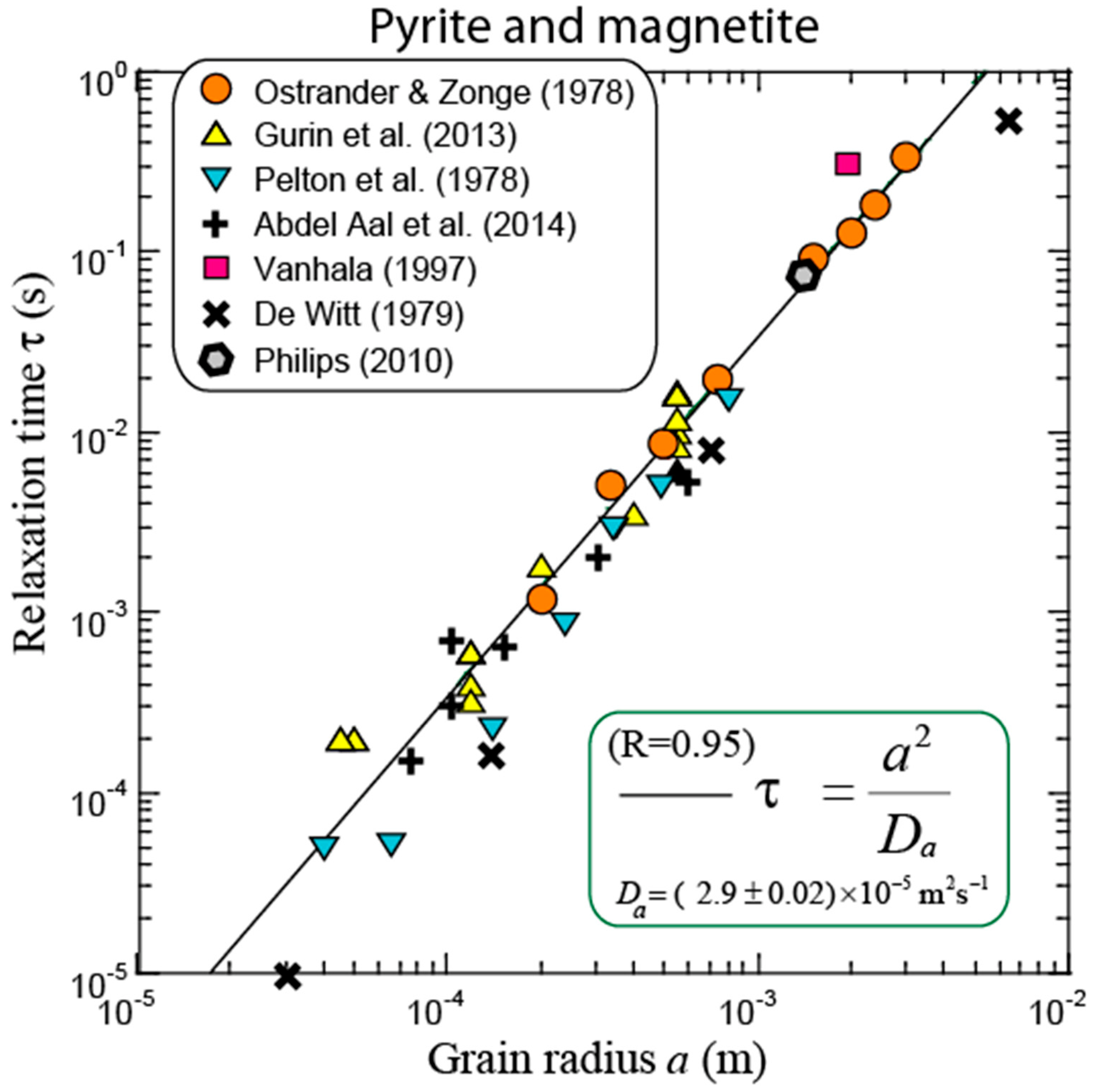
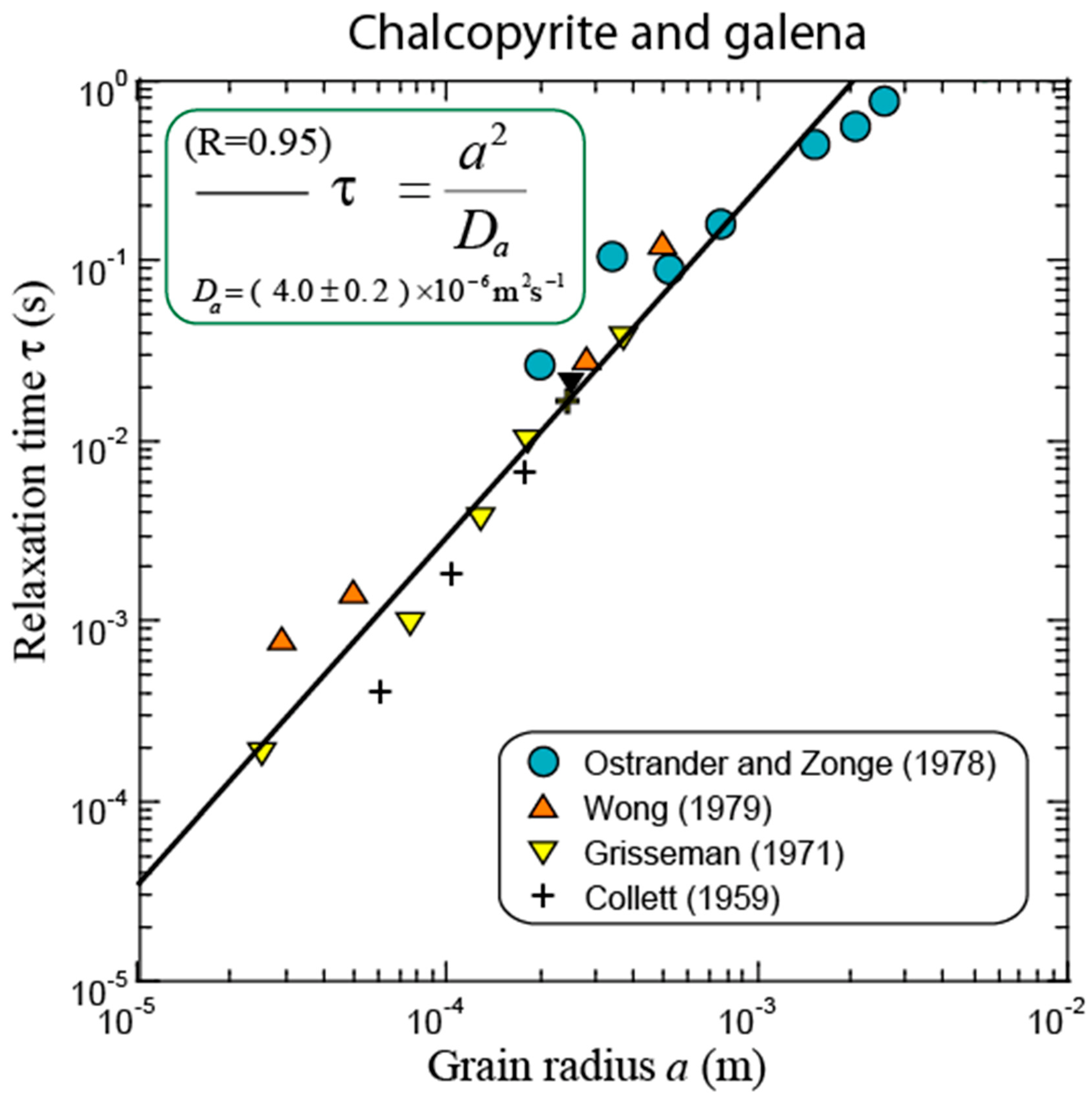
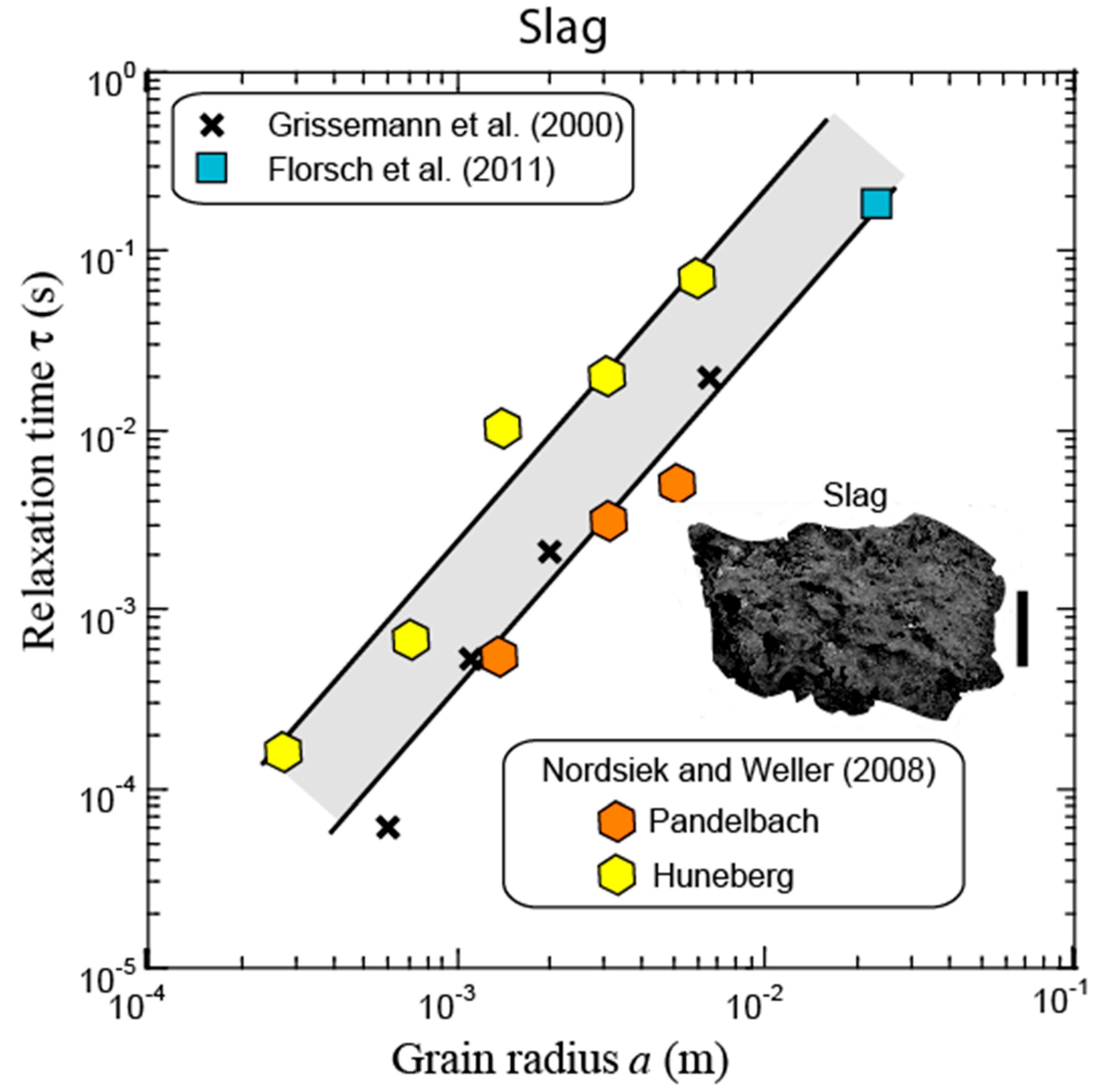
5.1. Relaxation Time

Our first goal is to test the relationship ${\tau }_0=a^2/D_a$. The relaxation time for the complex conductivity that is characterized by a low chargeability (<0.10) can be plotted as a function of the radius of the metallic grains (Figure 14 and Figure 15). The values of the apparent diffusion coefficient (D_a) that is found in Figure 15 (2.9 × 10⁻⁵ m² s⁻¹ at 25 °C, consistent with Olhoeft, 1983 [13]) and Figure 16 (4.0 × 10⁻⁶ m² s⁻¹ at 25 °C) are very high and are incompatible with the diffusion coefficient of the ions (typically ~1 × 10⁻⁹ m² s⁻¹ at 25 °C). The data that are shown in Figure 14 and Figure 15 indicate clearly that the relaxation time is proportional to the square of the grain radius (${\tau }_0\sim a^2$). This is true as long as the conductivity of the background material is constant (otherwise, see Figure 12).

Figure 16 shows a set of data for slag heap. Because we expect slags to be metallic electronic conductors (rather than semiconductors), we expect to see a higher diffusion coefficient for slag in comparison to pyrite and magnetite. With that being said, slag heaps also contain some small amounts of magnetite since they are characterized by some of the non-negligible values of their magnetic susceptibility [17]. Additional data are required to see if the trend that is shown in Figure 16 is general or not for non-glassy slags.

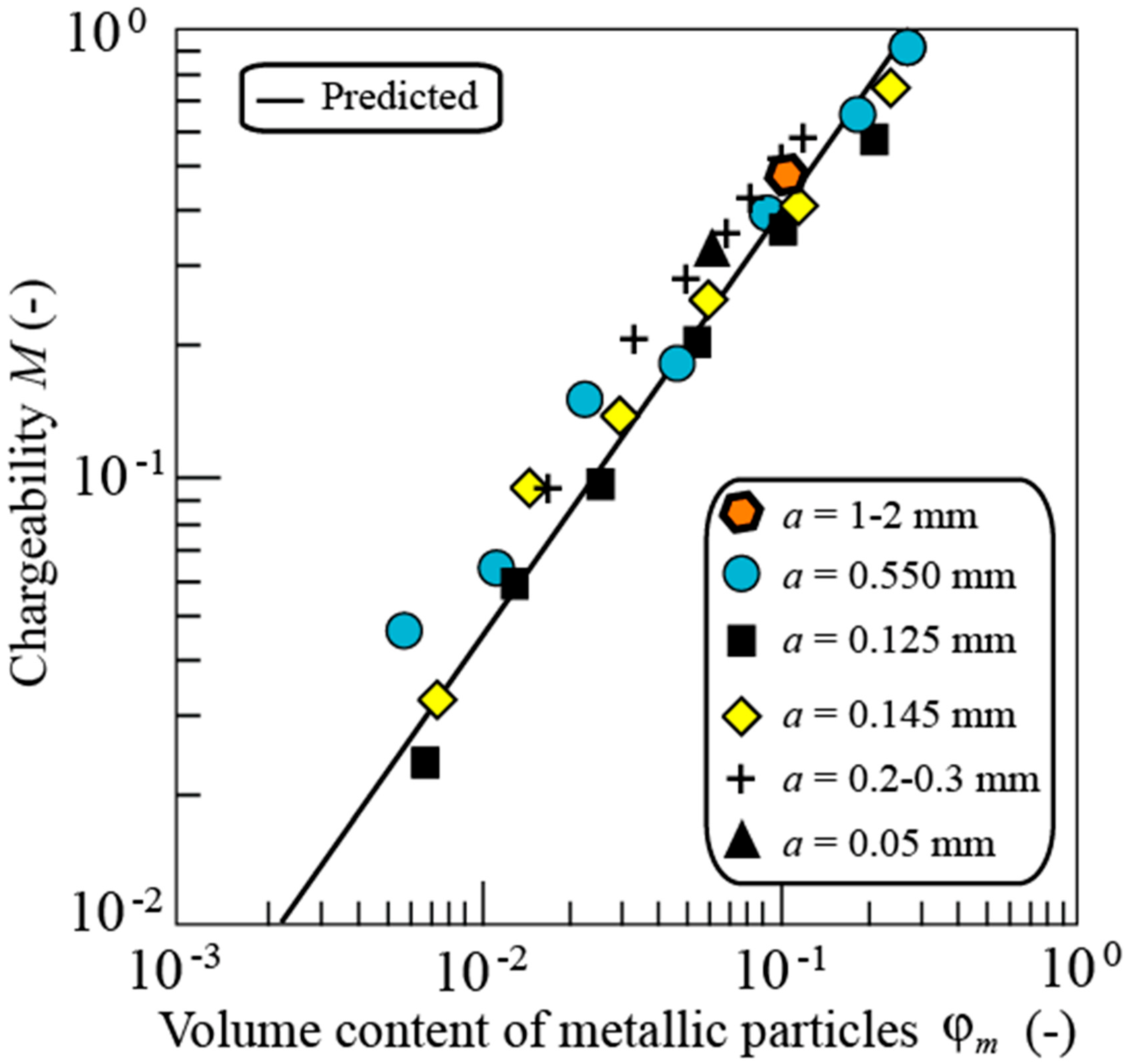
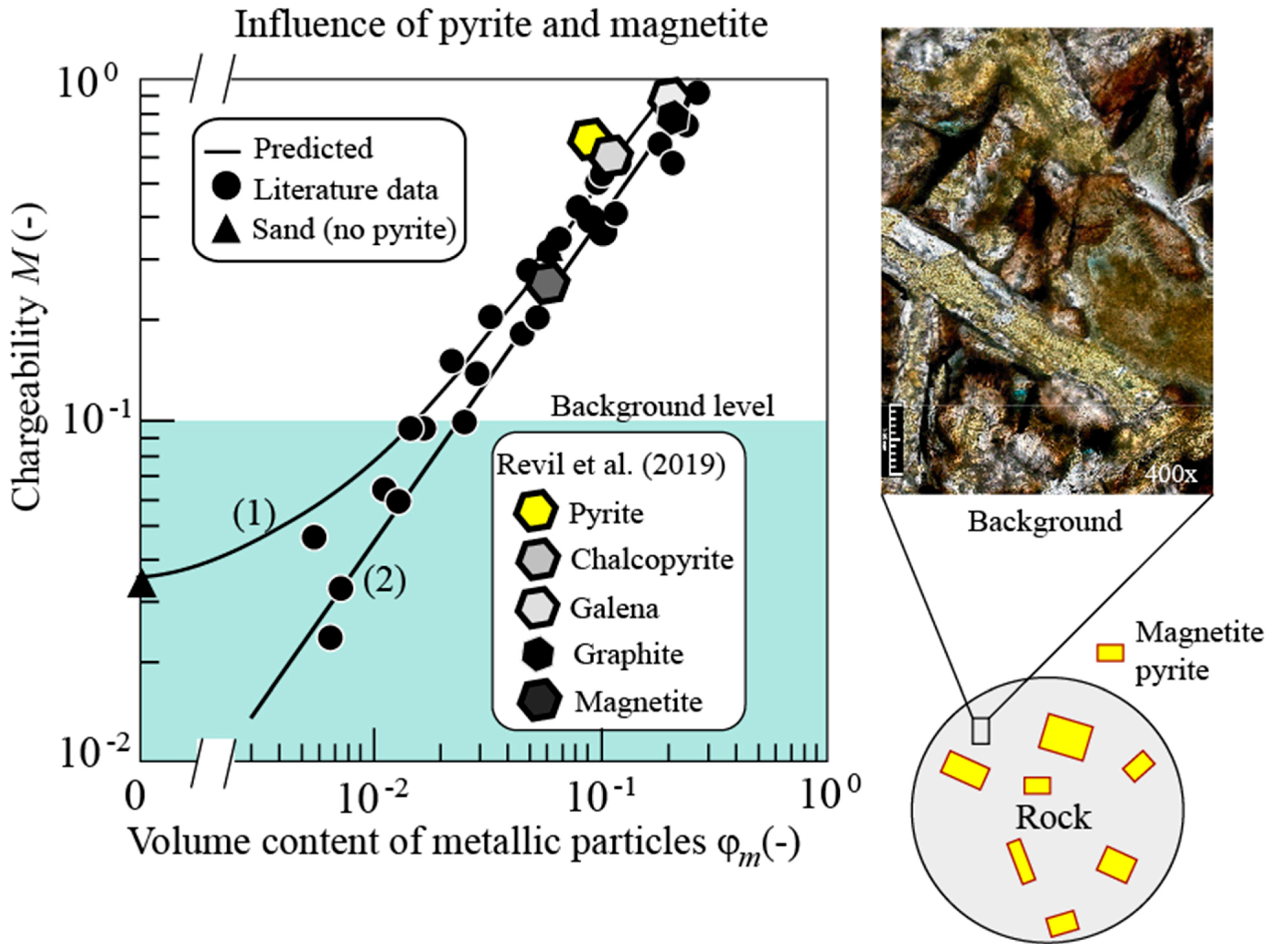
5.2. Chargeability and Volume Content of Metallic Particles

Equations (10) and (11) imply that the chargeability is a simple and direct indicator of the volumetric amount of the metallic particle in the pore space of the material (e.g., $M=(9/2){\phi }_m$,where ${\phi }_m$ denotes the volumetric content of the metallic particles). This relationship is independent of the radius of the metallic particles, and it is independent of the physico-chemistry of the pore water. This relationship is not affected much by the true shape of the metallic particles, as long as the particles are spheroids with an eccentricity that is smaller than 10 and as long as they are randomly oriented [47]. Figure 13 shows a comparison between the prediction of our model (plain line) and a variety of experimental data.

Figure 13 shows very clearly that the relationship between the chargeability and the volume content of metallic particles is mostly linear and is independent of the grain radius (a) of the metallic particles (at least for concentrations of semiconductors < 22% vol.). For metallic particle concentrations higher than 22%, the chargeability reaches a plateau that is close to 1. Figure 17 and Figure 18 show the effect of the content of metallic particles on the resistivity and chargeability, with fairly good agreement between the prediction of the proposed model and the laboratory data. Finally, the proposed model also predicts that the chargeability is independent of the pore-water conductivity, which is in agreement with the observations that were made by Clavier et al. (1976) [21].

6. Forward and Inverse Modeling

6.1. Classical Approach

In time-domain induced polarization, the apparent resistivities are determined by using the electrical potential that is recorded during the injection of the primary current through the current electrodes (A, B). The voltage response ($\psi$), which is due to the known point current source and Sinks A and B (at positions $r_{(\pm )}$, with current intensity ±$I$) can be described by the following elliptic partial differential equation that is obtained by combining Ohm’s law with a conservation equation for the charge in the quasistatic limit of the Maxwell equations:

$$\nabla \cdot ({\sigma }_{\infty }\nabla {\psi }_{\infty })=-I\left[\delta (r-r_{(+)})-\delta (r-r_{(-)})\right]$$

(53)

where $\delta (.)$ denotes the Dirac (delta) function (in m⁻³).

The ground surface ($\partial \Omega$) being insulating, the normal component of the electrical field vanishes, and therefore:

$${\left.\frac{\partial {\psi }_{\infty }}{\partial \widehat{n}}\right|}_{\partial \Omega }=0$$

(54)

where σ is the local electrical conductivity (in S m⁻¹), and $\widehat{n}$ is the unit vector normal to $\partial \Omega$. The apparent resistivity data can be inverted first by using an iterative Gauss–Newton algorithm by minimizing a cost function that is composed of a data misfit term and a regularizer, as discussed below.

Once the apparent resistivity data have been inverted, we can use the effect of the chargeability on the apparent chargeability, as discussed by Seigel (1959) [81], to invert the chargeability. As discussed above, induced polarization can be described by a macrscopic parameter that is called “chargeability” (M) [0, 1] (unit in V/V but usually expressed in mV/V). When the porous material is chargeable, the steady-state conductivity of the ground decreases with respect to the instantaneous conductivity, according to ${\sigma }_0={\sigma }_{\infty }(1-M)$ (the charges responsible for polarization do not contribute to conduction anymore). Equation (7) can be used to rerun the conductivity to obtain a new potential value (ψ) (Figure 1). We could define the apparent chargeability ($M_a$) as $M_a=({\psi }_0-{\psi }_{\infty })/{\psi }_0$. During the inversion, the log of the apparent chargeability is treated as the observed data that characterizes the polarization of the subsurface. The log of the chargeability is treated as the model parameter for each cell.

For the resistivity and chargeability problems, we can optimize an objective or cost function written as:

$$P^{\lambda }(m)={‖W_d(d(m)-d_{obs})‖}^2+\lambda {‖W_{m}m‖}^2$$

(55)

where the vector (m) is the model vector by using the log of the resistivity (or conductivity) and the chargeability for each cell, which are used to discretize the subsurface in order to enforce positiveness. The matrix W_d denotes the observation-data-weighting matrix that contains the uncertainties in the data (apparent resistivities or apparent chargeabilities). We can apply a first-order gradient matrix for the regularization matrix (W_m), or we can look for a smooth model by penalizing the roughness of the model vector. The regularization parameter (λ) is used to balance the influence between the data misfit and the regularizer in the objective function, and there are various ways to optimize this parameter during the iterative inversion process. The observation vector (d_obs) corresponds to the observed logarithm of the apparent resistivities or chargeabilities.

Following the classical algorithm that was developed by Oldenburg and Li (1994) [97], we use a deterministic inversion method with Tikhonov regulation to obtain a tomogram of the resistivity or chargeability. The intrinsic resistivity and chargeability are iteratively updated with:

$${\mathsf{m}}_{k+1}={\mathsf{m}}_k+\delta \mathsf{m}$$

(56)

where the perturbation is given by:

$$\delta m=-{\left[G^T(W_d^T{W}_d)G+\lambda W_m^T{W}_m\right]}^{-1}[G^T(W_d^T{W}_d)(d(m_i)-d_{obs})+\lambda W_m^T{W}_m{m}_k]$$

(57)

The vector δm provides the update of the vector m at iteration k. In this formulation, the matrix (G) denotes the sensitivity matrix, which is updated at each iteration. A benchmark of such an algorithm is provided in Figure 19. The upper two figures denote the true model (for resistivity and chargeability), while the two lower figures denote the inverted tomograms that are obtained by simulating an acquisition survey at the ground surface.

6.2. Source Current Approach

In time-domain induced polarization, the secondary voltage is associated with a secondary current, as discussed above in Section 3.2. The occurrence of the source of the current in the absence of an external applied electrical field is similar to a self-potential problem. Indeed, in geophysics, the self-potential method is a passive geophysical method in which the electrical field is passively measured at the surface of the Earth and is associated with the existence of current sources in the ground. After the shutdown of the primary current, a total current density (J) (in A m⁻²) can be described by a generalized Ohm’s law:

$$J=\sigma E+J_S$$

(58)

where E denotes the secondary electrical field (in V m⁻¹), and J_S is the secondary (source) current density that is responsible for the observed electrical field (in A m⁻²). Since the time variation of the current density is very slow, we can use the quasistatic limit of the Maxwell equations, for which the conservation of the charge takes the form:

$$\nabla \cdot J=0\hspace{0.17em}$$

(59)

By combining Equations (59) and (60), the scalar electrical potential ($\psi$) is the solution of a Poisson equation:

$$\nabla \cdot (\sigma \nabla \psi )=\nabla \cdot J_s$$

(60)

Therefore, Equation (61) is both the classical self-potential equation and the equation that describes the secondary electrical potential fluctuations in time-induced polarization after the shutting down of the primary current or the electrical field. The electrical potential solution of Equation (61) can also be written in an integral form, which, once discretized, can, in turn, be written as:

$$\mathsf{d}=\mathsf{K}\mathsf{m}$$

(61)

The (N×M)-matrix (K) denotes the kernel, which is the collection of the Green’s function for the electrical potential problems, and which is obtained by putting the element-source current densities of the unit strength into the three main directions for each cell that is used to discretize the subsurface; $\mathsf{d}$ is an N-vector in the collection of recorded electrical potentials at the N-electrodes; and m is an M-vector that corresponds to the source current-density times the volume of each cell (therefore, each element of m is expressed in A m) for the M-cells that are used to discretize the volume of interest. Alternatively, the integration volume could be accounted for in the elements of the kernel. Since the elements of the kernel should account for the boundary conditions and the complicated electrical-conductivity distribution, we cannot use analytical solutions for the Green’s functions. We compute them numerically with the finite element software Comsol Mutiphysics 4.0 by placing elementary dipoles in the three principal directions: x, y, and z.

The secondary voltage decays are treated as an N-observed data vector (d_obs) at each time following the shutdown of the primary current. The objective function to minimize is defined as:

$$P^{\lambda }(\mathsf{m})={‖W_d(K\mathsf{m}-{\mathsf{d}}_{obs})‖}^2+\lambda {‖W_m\mathsf{m}‖}^2$$

(62)

In this equation, W_m denotes a matrix that is used to regularize the inverse problem. Equation (63) can be minimized, and the optimized model vector can be obtained in a single iteration as:

$$\mathsf{m}={\left[K^T(W_d^T{W}_d)K+\lambda (W_m^T{W}_m)\right]}^{-1}\cdot \left[K^T(W_d^T{W}_d){\mathsf{d}}_{obs}\right]$$

(63)

Various approaches are used to focus the source current densities and to properly normalize the model vector to avoid favoring sources that are close to the ground surface (see details in Soueid Ahmed and Revil, 2018 [99]). Figure 20 shows a tomography of the Cole–Cole parameters for an anomalous polarizable body in a tank [99]. This approach is very robust and fast, and especially because we solve a linear problem.

Figure 21 shows, for instance, that the normalized chargeability and the quadrature conductivity can be related to each other. This linear relationship allows for the conversion of the time-domain acquired date to complex conductivity data. If time-domain measurements are performed at different periods, we can even reconstruct complex conductivity spectra in a very simple way.

6.3. Tomography of the Relaxation Time

Our goal in this section is to show that we can easily perform a tomography of the main relaxation time by performing two tomographies of two distinct chargeabilities. First, it is worth mentioning that equivalent electrical circuits have been also broadly used to model the induced-polarization voltage-decay patterns in time-domain induced polarization. For the sake of simplicity, we consider the simplest circuit, which is, namely, an RC circuit (R and C stand for resistance and capacitance, respectively, see Figure 22).

Charging this circuit first with the normalized unit voltage, and then switching off the circuit leads to a decay in the secondary voltage, as:

$$\mathsf{\psi }(t)=\frac{{\mathsf{R}}_1}{{\mathsf{R}}_1+{\mathsf{R}}_2}\exp \left(-\frac{t}{({\mathsf{R}}_1+{\mathsf{R}}_2)\mathsf{C}}\right)=M e^{-\frac{t}{\tau }}$$

(64)

The quantity $\psi (t)$ describes the difference in the potential between the voltage electrodes (M and N); C is the capacitance; R₁ and R₂ are the two resistances shown in Figure 22; and the chargeability is given by $M={\mathsf{R}}_1/({\mathsf{R}}_1+{\mathsf{R}}_2)$ (dimensionless). The relaxation time of the circuit, which is shown in Figure 22, is given by $\tau =({\mathsf{R}}_1+{\mathsf{R}}_2)\mathsf{C}$. We have the following properties: $0\le M\le 1$ and $0\le \tau <+\infty$. The spectral response relative to this model can be obtained by injecting a harmonic current into the circuit, as shown in Figure 22. The associated impedance can be easily determined, and the associated complex resistivity corresponds to the so-called “Debye response”, which is written as:

$$\mathsf{\rho }*=\frac{1}{\sigma *}={\mathsf{\rho }}_0\left[1-M\left(1-\frac{1}{1+\mathsf{i}\omega \tau }\right)\right]$$

(65)

where $M=({\mathsf{\rho }}_0-{\mathsf{\rho }}_{\infty })/{\mathsf{\rho }}_0$ is the chargeability, and ${\mathsf{\rho }}_0$ and ${\mathsf{\rho }}_{\infty }$ denote the apparent resistivities at the null frequency (continuous or direct current (DC condition)) and at an infinite frequency, respectively, and which is also called the “instantaneous resistivity” (${\mathsf{\sigma }}_0=1/{\mathsf{\rho }}_0$ and ${\mathsf{\sigma }}_{\infty }=1/{\mathsf{\rho }}_{\infty }$). The null frequency means that the current would be applied for an infinite time and that all of the polarization phenomena in the material have reached steady-state conditions in a thermodynamic sense. To enforce that the chargeability (M) in Equation (66) is the same as in Equation (65), we first write Equation (66) as:

$$\frac{{\mathsf{\rho }}^{*}(\omega )}{{\mathsf{\rho }}_0}=(1-M)+M\left(\frac{1}{1+\mathsf{i}\omega \tau }\right)=\frac{\tilde{\mathsf{\psi }}*(\omega )}{{\mathsf{\psi }}_0}$$

(66)

where $\tilde{\mathsf{\psi }}*$ denotes the complex potential that is proportional to the complex resistivity, through Ohm’s law, in the Fourier domain. Taking the inverse Fourier transform provides the impulse response of this filter, precisely as:

$$\mathsf{h}(t)=\mathsf{F}{\mathsf{T}}^{-1}\left[\frac{\tilde{\mathsf{\psi }}*(\omega )}{{\mathsf{\psi }}_0}\right]$$

(67)

$$\mathsf{h}(t)=\mathsf{F}{\mathsf{T}}^{-1}\left[(1-M)+M\left(\frac{1}{1+\mathsf{i}\omega \tau }\right)\right]$$

(68)

$$\mathsf{h}(t)=(1-M)\delta (t)+M\tau {\mathsf{e}}^{-\frac{t}{\tau }}$$

(69)

where FT⁻¹ denotes the inverse Fourier transform. The response to a unit step is obtained by the integration of this impulse response, and it would correspond to the time that the current is just sent, which passes from 0 to +1, and from t = 0. We obtain, in the time domain, the following voltage-decay response:

$$\frac{\mathsf{\psi }(t)}{{\mathsf{\psi }}_0}={\displaystyle {\int }_0^t\mathsf{h}(t)dt=1-M{\mathsf{e}}^{-\frac{t}{\tau }}}$$

(70)

When discharging (that is, after switching off the injected current), we just obtain the decaying-potential ratio: $\mathsf{\psi }(t)/{\mathsf{\psi }}_0=M\exp (-t/\tau )$.

Another chargeability was defined in the realm of the mining industry and it is called the “integral chargeability” (expressed in s), which is defined as:

$$\widehat{\mathsf{M}}=\frac{1}{{\mathsf{\psi }}_0}{\displaystyle {\int }_0^{\infty }\mathsf{\psi }(t)}dt$$

(71)

$$\widehat{\mathsf{M}}={\displaystyle {\int }_0^{\infty }\mathsf{M}{\mathsf{e}}^{-\frac{t}{\tau }}}\mathrm{dt}=\mathsf{M}\tau$$

(72)

In other words, in the context of the electrical circuit that is shown in Figure 22, the relaxation time (τ) is the ratio of the integral chargeability by the chargeability. This relation is also valid for a Cole–Cole model instead of a Debye model (Florsch, personal communication 2019). In terms of the tomography, we can therefore perform a tomography of the integral chargeability according to one of the approaches underlined above, and a second chargeability tomography by using the classical apparent chargeability. Then, cell by cell, the relaxation time is obtained by dividing the inverted integral chargeability by the chargeability. We will show one example of the relaxation-time tomography that was obtained by using this approach in the next section in the context of a metallic tank (Section 7.4).

7. Applications

7.1. Treasure Quest: Finding Pyrite in a Sandbox

The first test of the method is to use electrical-resistivity tomography and induced polarization to find an area that is rich in pyrite cubes in a sandbox experiment. The sandbox is saturated with tap water. The results that are shown in Figure 23 indicate that the electrical-conductivity distribution is not sensitive enough to show the position of the disseminated pyrite cubes, while the induced polarization clearly shows where the ore is located (Figure 24). This is consistent with our model, for which the presence of ore has only a second-order effect on the conductivity distribution, while the volume content of the ores directly controls the chargeability of the material. Furthermore, at low frequencies, the pyrite cubes would appear to be insulators that increase the resistivity of the material (Figure 17). The observation of resistive bodies inside a more conductive background is inherently difficult. Figure 25 shows the results of another set of sandbox experiments that used a target that was composed of sand mixed with pyrite and bentonite. The targets were immersed in a sand background. The sandboxes were saturated with tap water. These experiments confirm the previous findings and show that, for bentonite, it is better to use the normalized chargeability to show up the target because of its high cation exchange capacity (CEC).

7.2. Treasure Quest: Finding Slag at an Archeological Site

Dumped slag heaps that have been used over the history of humankind can be seen as valuable deposits to feed the growing need for metal resources. As shown in the previous section, the spatial delineation of slag heaps cannot easily be obtained from the resistivity distribution. The induced-polarization method can be used to fulfill this goal. A least-square 3D induced-polarization inversion based on the least-square technique is used to obtain the chargeability distribution that delimits a slag heap at the archeological site of Saint-Vincent sur L’Isle, Dordogne, France (Figure 26). From the linear relationship that is determined between the chargeability and the volumetric metal content, the metallic volume of the slag heaps can be directly determined. A volume of high chargeability (above the background value of 0.08) indicates the position of the slag heap. The linear relationship between the chargeability and the metallic volumetric content (see Figure 14) is used to provide an image of the distribution of the metals that are present at this archeological site (Figure 27).

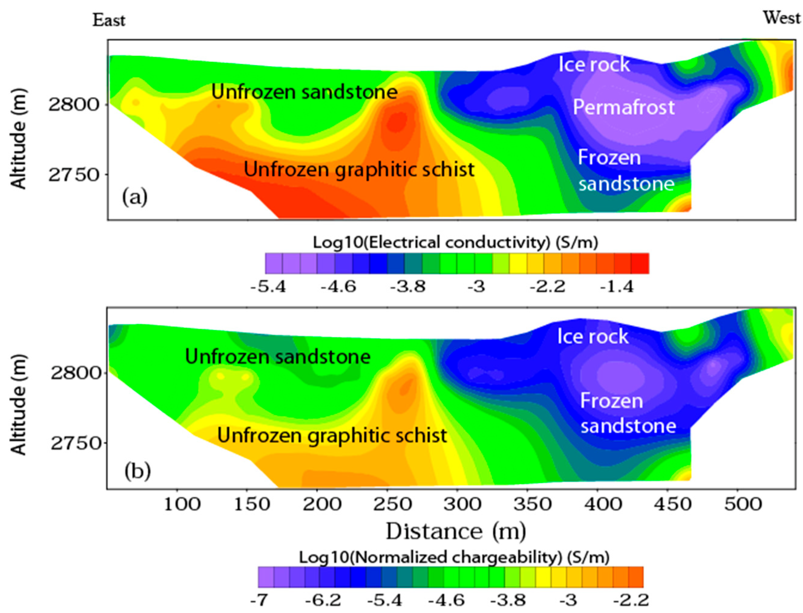
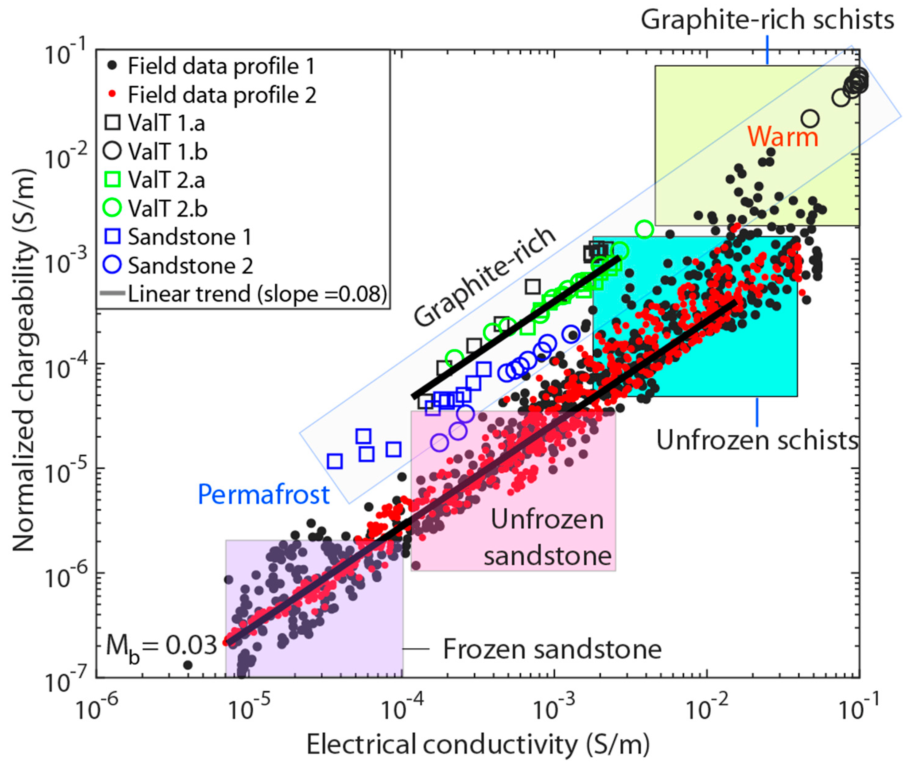
7.3. Graphitic Schists and Permafrost

This section demonstrates the effects of the temperature below the freezing point on rocks that contain metals, with an application to graphitic schists. Spectral induced polarization spectra performed with graphite graphitic show a very strong effect of temperature below the freezing point (see Figure 28). Since the temperature has a strong effect on the instantaneous conductivity, it is not surprising, in the framework of the model discussed above, that the relaxation time is also dependent on the instantaneous conductivity and on the temperature (Figure 29). As long as the temperature decreases, the electrical conductivity decreases, and the relaxation time increases. Figure 30 and Figure 31 demonstrate the effects of both graphite and temperature on the electrical conductivity and chargeability tomography.

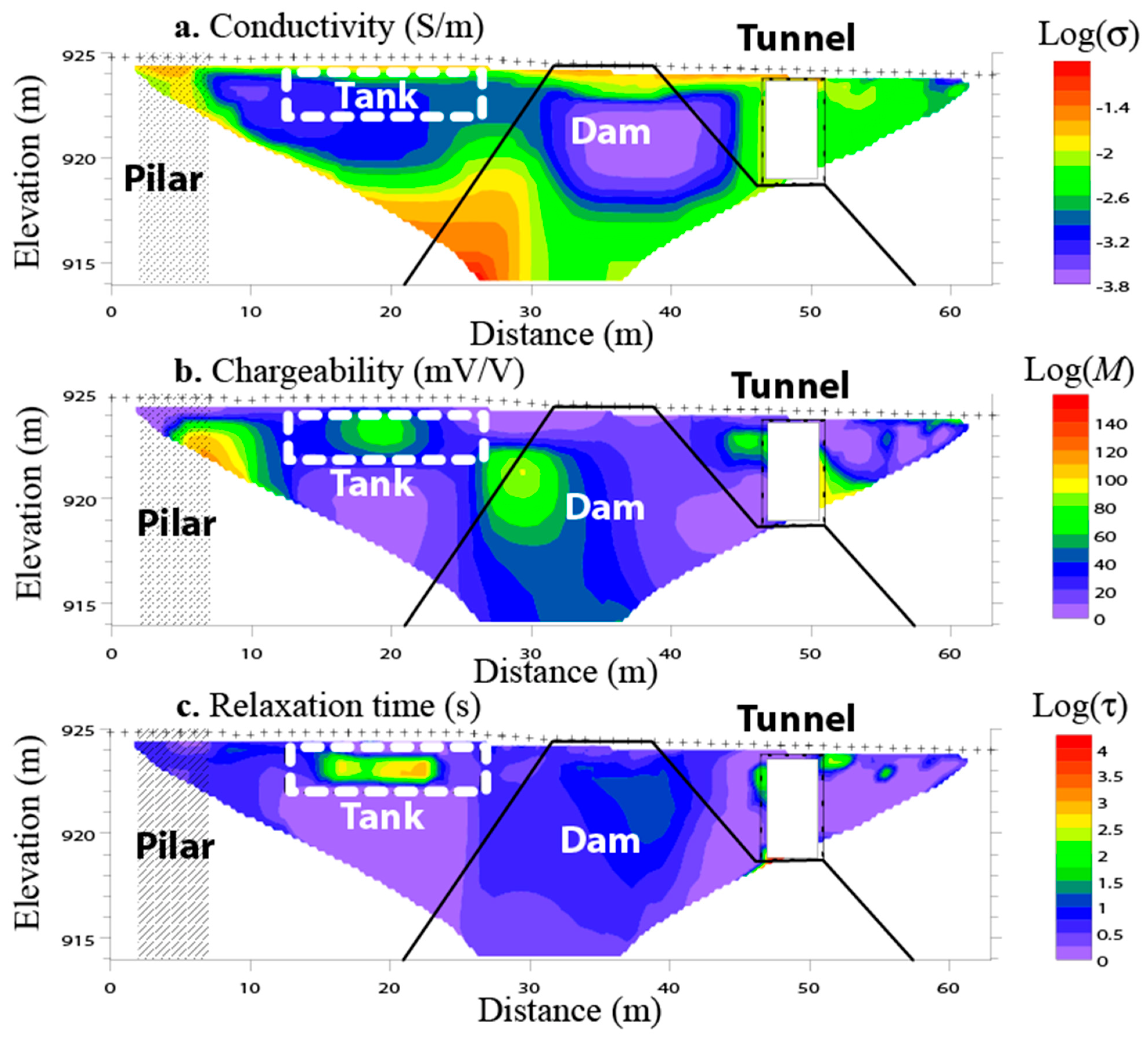
7.4. Localization of a Metallic Tank

We illustrate now the use of a relaxation-time tomography to perform a tomography of a metallic tank underground (see Section 6.3 above). This case study is illustrated in Figure 32. We see that both the chargeability and the relaxation-time tomography can be used to detect a metallic tank. The tomography of the relaxation time provides a very clear image of the tank.

7.5. Application to a Deep Cu–Pb–Zn Deposit

Although the traditional induced polarization method in the time and frequency domains [28,52,53,54,55] has achieved great successes, it cannot necessarily meet the needs of large-scale induced-polarization exploration in the presence of strong electromagnetic interferences. The idea that underlies spread-spectrum communication [101] was introduced into induced-polarization instrumentation by Xi et al. (2013, 2014) [102,103] and their corresponding data processing. Liu et al. (2016, 2017) [104,105] proposed a spread-spectrum induced-polarization (SSIP) method that is based on ZigBee wireless sensor networks and GPS timing to realize synchronous real-time full-waveform acquisition and the real-time data-quality monitoring of massive SSIP receivers [103,106]. At the same time, the GPS timing and synchronization of the SSIP transmitter and the spread-spectrum IP receiver, as well as the ZigBee wireless networking of the spread-spectrum IP transmitter, the receiver array, and the personal computer (control center) are realized [103]. On the basis of these technologies, exploration depths greater than 1000 m, even in the presence of strong electromagnetic interferences, could be achieved [105,107,108].

In order to showcase a proof of concept of such an exploration tool, it was applied to a Cu–Pb–Zn polymetallic mine in Baiyin City, Gansu Province, China. The silver–copper–lead–zinc polymetallic deposit belongs to the VMS (volcanogenic massive sulfide) deposits, which was once the largest copper mine in China and which has a mining history of hundreds of years [109]. The exploration section is located west of the ore body that is being mined underground. Because of the existence of strong electromagnetic interferences, such as underground mineral mining, mineral-processing plants, and smelters around the profile, it is extremely challenging to achieve an IP exploration depth of 1000 m. In order to realize the high-resolution exploration of SSIP at depths higher than 1000 m, 25 sets of four-channel SSIP receivers were used for synchronous observation, which achieved a minimum measurement dipole spacing of 20 m, and which covered a profile length of 2000 m. In order to achieve high-resolution exploration, the observation starts from the minimum distance of 20 m from the supply electrode, and the center of the supply dipole is the center of the survey line. Then, increase the power-supply dipole distance by 80 m each time inside the survey line. To the outside of the survey line, increase the power-supply dipole distance by 400 m each time until the maximum power-supply dipole distance is 5200 m (Figure 33). Each time that power is supplied, the 25 receivers start observing simultaneously.

There are various electromagnetic interferences in the measured waveforms. Considering the short-term and random nature of electromagnetic interferences, robust superposition and correlation detection are used to enhance the signal-to-noise ratio [104,105]. Considering that the maximum power-supply dipole distance is 5200 m, there is also electromagnetic coupling induction in the measurement results. Therefore, the relative phase spectrum is used to suppress the influence of electromagnetic coupling interference [110].

Figure 34 shows the resistivity-and-chargeability (relative phase is converted into chargeability in the inversion) profile after the inversion using ZondRes2D, as well as the Cu–Pb–Zn-ore-body morphology that was verified by drilling. From the resistivity profile in the figure, the existence of a steeply standing fault can be roughly inferred, but the existence of an ore body cannot be inferred. Fortunately, an oblong polarizability anomaly can be found from the polarizability profile of the figure. The location of the chargeability anomaly is consistent with the fault location, which is implied in the resistivity profile, so that it can be reasonably inferred that the IP anomaly is caused by the VMS ore body. Subsequent drill holes have verified the above inferences, and the IP anomaly that was discovered this time is highly consistent with the verified VMS ore body.

8. Future Trends in Marine Exploration

In this section, we want to discuss the possible integration of the electrical conductivity/inducedpolarization methods with the self-potential technique. The self-potential method is a passive geophysical technique that measures the electrical field that is associated with the natural source of the currents in the subsurface [111]. Induced-polarization surveys can be performed at the seafloor [112]. Negative self-potential (SP) anomalies near seafloor massive sulfide deposits are associated with redox-active environments, in which metallic bodies are located [113].

Recently, self-potential surveys were used to investigate SMS (seafloor massive sulfides) deposits at the seafloor. The inversion of the self-potential data can be used to obtain a 3D tomogram of the causative-source-current density, which, in turn, can underline the ore body [114]. Meanwhile, a self-potential survey uses very simple equipment (nonpolarizing electrodes and a sensitive voltmeter), which can be easily mounted together with active (galvanometric or induction-based) sensors to image the resistivity and the induced polarization [115].

In order to show the new capabilities of the self-potential method, we discuss here two case studies. Zhu et al. (2020) [115] conducted a combined self-potential and transient electromagnetic survey on the southwest Indian ridge. Six horizontal AgCl electrodes were attached to the transient electromagnetic system to passively record the horizontal electrical-field component (Figure 35). The natural electrical field was extracted from the raw data and was integrated to obtain the self-potential signals. Negative self-potential anomalies (~−27 mV) were observed at the known Yuhuang hydrothermal field. The inversion of these self-potential data reveals localized SMS deposits with a thickness of ~65 m (Figure 36).

The second case study is reported by Kasaya et al. (2020) [116], who conducted a self-potential and marine direct-current-resistivity survey by using two autonomous underwater vehicles (Figure 37 and Figure 38). The self-potential and the apparent resistivity were obtained along a survey line that crossed the known hydrothermal mounds of sulfide ore in the mid-Okinawa Trough. Similar to the previous case study, the raw self-potential data were integrated to obtain a potential field profile. The distribution of the negative self-potential anomalies obtained and the low apparent resistivity (0.2 ohm-m or less) show good agreement with the locations of the known hydrothermal deposits (Figure 39).

Recent studies have demonstrated that self-potential tomography can play an important role in the exploration of SMS deposits. However, the electrical-conductivity distribution of SMS deposits is an important ingredient in the inversion of the recorded self-potential data. Indeed, the self-potential governing equation is given as [111]:

$$\nabla \cdot (\sigma \nabla \phi )=\nabla \cdot {\mathsf{J}}_s$$

(73)

where σ denotes the electrical conductivity, $\phi$ is the self-potential field, and ${\mathsf{J}}_s$ denotes the source-current density that is associated with the ore body. We can develop the left-hand side to obtain [117]:

$${\nabla }^2\phi =\frac{\nabla \cdot {\mathsf{J}}_s}{\sigma }+\nabla \ln \sigma \cdot \mathsf{E}$$

(74)

where $\mathsf{E}=-\nabla \phi$ is the electrical field. Equation (74) shows that, in order to obtain the source-current density, knowledge of the conductivity distribution ($\sigma$) below the seafloor is required [111,118]. Future analysis must combine induced-polarization tomography with the inversion of the self-potential data in order to better quantify SMS deposits.

9. Conclusions

We have reviewed a physics-based model that describes the complex conductivity of porous materials that contain disseminated metallic particles. This model is based on the intrinsic polarization of the metallic grains, in which the charge carriers accumulate at the boundary of the grains. This model can be applied to characterize metallic deposits by using a geophysical technique that is called “induced polarization”. The chargeability depends on the volumetric content of the metallic particles plus the chargeability of the background material. The relaxation time depends on the square of the radius of the metallic grains and it is inversely proportional with respect to the conductivity of the background material, which is weakly dependent on the volume fraction of the metallic particles. The DC conductivity decreases with the increase in the concentration of the metallic particles, while the high-frequency conductivity increases with the concentration of metallic particles. This statement may appear obvious from the fact that the grains act as conductors at high frequencies (absence of polarization) and as insulators at low frequencies (grains totally polarize). With that being said, this point is often forgotten by the practitioners of electromagnetic methods when dealing with the dependence of the electrical conductivity on the fraction of metallic particles. In other words, conduction is not just an electromigration problem, and it cannot be fully understood without its counterpart that corresponds to the grain polarization. We have not discussed the potential effect of redox reactions at the grain/water interface, but such an effect would make the metallic grains leaking capacitors rather than perfect capacitors, as described in this paper.

We have discussed five applications and tests of the petrophysical model that use induced-polarization tomography, including conductivity, chargeability, and relaxation-time tomography. Our tests demonstrate that electrical-conductivity tomography is not efficient at imaging disseminated ores. In time-domain induced polarization, the secondary voltage decay can be understood as a transient self-potential problem. The relaxation-time tomography is efficient at imaging massive metallic structures. We also show that the effect of temperature, including the effect of permafrost, is well understood and can be used to interpret field data. An exploration case shows that, on the basis of the spread-spectrum-communication idea and the array SSIP signal acquisition that is based on ZigBee and GPS timing, high-resolution induced-polarization exploration at depths of ~1000 m, even in the presence of strong electromagnetic interferences, can be realized. Further works will need to be conducted to perform the joint inversion of induced-polarization data with self-potential data to further image and localize SMS deposits below the seafloor.

References

1. Dahlin, T.; Leroux, V. Improvement in time-domain induced polarization data quality with multi-electrode systems by separating current and potential cables. Near Surf. Geophys. 2012, 10, 545–565. [Google Scholar] [CrossRef] [Green Version]
2. Schlumberger, C. Etude sur la Prospection Electrique du Sous-Sol, Gauthier-Villars, Paris. The Second Edition without Modification Is Available at https://gallica.bnf.fr/ark:/12148/bpt6k64569898.texteImage. English Version, Translated by Sherwin F. Kelly: “Study of Underground Electrical Prospection”. Available online: https://archive.org/details/studyofundergrou00schlrich/page/n37 (accessed on 24 April 2022).
3. Li, J.L. Application of the down-hole IP method to a general survey in the Jinya gold deposit. Geol. Explor. 2016, 2016, 924–930. (In Chinese) [Google Scholar]
4. Dakhnov, V.N.; Latyshova, M.G.; Ryapolova, V.A. Investigation of drill holes by the method of induced potentials. Promysl. Geofiz. 1952, 1952, 46–82. [Google Scholar]
5. Marshall, D.J.; Madden, T.R. Induced polarization, a study of its causes. Geophysics 1959, 24, 790–816. [Google Scholar] [CrossRef]
6. Olhoeft, G.R. Low-frequency electrical properties. Geophysics 1985, 50, 2492–2503. [Google Scholar] [CrossRef]
7. Weiss, O. The limitations of geophysical methods and the new possibilities opened up by an electrochemical method for determining geological formations at great depths, World Pet. Congr. London Proc. 1933, 1, 114–118. [Google Scholar]
8. Wait, J.R. Overvoltage Research and Geophysical Applications; Pergamon: London, UK, 1959; Volume 4. [Google Scholar]
9. Bleil, D.F. Induced polarization: A method of geophysical prospecting. Geophysics 1953, 18, 636–661. [Google Scholar] [CrossRef]
10. Anderson, L.A.; Keller, G.V. A study in induced polarization. Geophysics 1964, 29, 848–864. [Google Scholar] [CrossRef]
11. Pelton, W.H.; Ward, S.H.; Hallof, P.G.; Sill, W.R.; Nelson, P.H. Mineral discrimination and removal of inductive coupling with multifrequency IP. Geophysics 1978, 43, 588–609. [Google Scholar] [CrossRef]
12. Hallof, P.G.; Klein, J.D. Characterization of electrical properties of metallic mineral deposits. Ont. Geol. Surv. Open File Rep. 1983, 1983, 5468. [Google Scholar]
13. Olhoeft, G.R. Electrical properties of rocks and minerals. Short Course Notes, Golden, CO, USA, 1983. [Google Scholar]
14. Vanhala, H.; Peltoniemi, M. Spectral IP studies of Finnish ore prospects. Geophysics 1992, 57, 1545–1555. [Google Scholar] [CrossRef]
15. Hallof, P.G.; Yamashita, M.; Fink, J.B.; Sternburg, B.K.; McAlister, E.O.; Wieduwilt, W.G. The use of the IP method to locate gold-bearing sulfide mineralization. In Applications and Case Histories; The Society of Exploration Geophysicists: Houston, TX, USA, 1990. [Google Scholar]
16. Fleet, M.E.; Mumin, A.H. Gold-bearing arsenian pyrite and marcasite and arsenopyrite from Carlin Trend gold deposits and laboratory synthesis. Am. Mineral. 1997, 82, 182–193. [Google Scholar] [CrossRef]
17. Florsch, N.; Llubes, M.; Téreygeol, F.; Ghorbani, A.; Roblet, P.J. Quantification of slag heap volumes and masses through the use of induced polarization: Application to the Castel-Minier site. J. Archaeol. Sci. 2011, 38, 438–451. [Google Scholar] [CrossRef]
18. Florsch, N.; Camerlynck, C.; Revil, A. Direct estimation of the distribution of relaxation times from induced-polarization spectra using a Fourier transform analysis. Near Surf. Geophys. 2012, 10, 517–531. [Google Scholar] [CrossRef] [Green Version]
19. Florsch, N.; Llubes, M.; Téreygeol, F. Induced polarization 3D tomography of an archaeological direct reduction slag heap. Near Surf. Geophys. 2012, 10, 567–574. [Google Scholar] [CrossRef]
20. Nordsiek, S.; Weller, A. A new approach to fitting induced-polarization spectra. Geophysics 2008, 73, F235–F245. [Google Scholar] [CrossRef]
21. Clavier, C.; Heim, A.; Scala, C. Effect of pyrite on resistivity and other logging measurements. In Proceedings of the SPWLA 17th Annual Logging Symposium, Denver, CO, USA, 9 June 1976. [Google Scholar]
22. Sternberg, B.K. A review of some experience with the induced-polarization/resistivity method for hydrocarbon surveys: Successes and limitations. Geophysics 1991, 56, 1522–1532. [Google Scholar] [CrossRef]
23. Veeken, P.C.; Legeydo, P.J.; Davidenko, Y.A.; Kudryavceva, E.O.; Ivanov, S.A.; Chuvaev, A. Benefits of the induced polarization geoelectric method to hydrocarbon exploration. Geophysics 2009, 74, B47–B59. [Google Scholar] [CrossRef]
24. Flekkøy, E.G.; Legeydo, P.; Håland, E.; Drivenes, G.; Kjerstad, J. Hydrocarbon detection through induced polarization: Case study from the Frigg area. In SEG Technical Program Expanded Abstracts; The Society of Exploration Geophysicists: Houston, TX, USA, 2013. [Google Scholar]
25. Okay, G.; Cosenza, P.; Ghorbani, A.; Camerlynck, C.; Cabrera, J.; Florsch, N.; Revil, A. Characterization of macroscopic heterogeneities in clay-rocks using induced polarization: Field tests at the experimental underground research laboratory of Tournemire (Aveyron, France). Geophys. Prospect. 2013, 61, 134–152. [Google Scholar] [CrossRef]
26. Hupfer, S.; Martin, T.; Noell, U.; Camerlynck, C.; Chauris, H.; Maineult, A.; Schmutz, M. Laboratory SIP: Investigation on unconsolidated mineral-sand mixtures. In Proceedings of the Third International Workshop on Induced Polarization, ENSEGID Bordeaux, Oléron Island, France, 6–9 April 2014; pp. 12–13. [Google Scholar]
27. Chen, J.; Hubbard, S.S.; Williams, K.H.; Flores Orozco, A.; Kemna, A. Estimating the spatiotemporal distribution of geochemical parameters associated with biostimulation using spectral induced polarization data and hierarchical Bayesian models. Water Resour. Res. 2012, 48, W0555. [Google Scholar] [CrossRef]
28. Orozco, A.F.; Kemna, A.; Oberdörster, C.; Zschornack, L.; Leven, C.; Dietrich, P.; Weiss, H. Delineation of subsurface hydrocarbon contamination at a former hydrogenation plant using spectral induced polarization imaging. J. Contam. Hydrol. 2012, 136, 131–144. [Google Scholar] [CrossRef] [PubMed]
29. Mewafy, F.M.; Werkema, D.D., Jr.; Atekwana, E.A.; Slater, L.D.; Aal, G.A.; Revil, A.; Ntarlagiannis, D. Evidence that bio-metallic mineral precipitation enhances the complex conductivity response at a hydrocarbon contaminated site. J. Appl. Geophys. 2013, 98, 113–123. [Google Scholar] [CrossRef]
30. Ntarlagiannis, D.; Williams, K.H.; Slater, L.; Hubbard, S. Low-frequency electrical response to microbial induced sulfide precipitation. J. Geophys. Res. Biogeosci. 2005, 110, G02009. [Google Scholar] [CrossRef] [Green Version]
31. Weller, A.; Börner, F.D. Measurements of spectral induced polarization for environmental purposes. Environ. Geol. 1996, 27, 329–334. [Google Scholar] [CrossRef]
32. Vacquier, V.; Holmes, C.R.; Kintzinger, P.R.; Lavergne, M. Prospecting for ground water by induced electrical polarization. Geophysics 1957, 22, 660–687. [Google Scholar] [CrossRef]
33. Martin, T. Complex resistivity measurements on oak. Eur. J. Wood Wood Prod. 2012, 70, 45–53. [Google Scholar] [CrossRef]
34. Cole, K.S.; Cole, R.H. Dispersion and absorption in dielectrics I. Alternating current characteristics. J. Chem. Phys. 1941, 9, 341–351. [Google Scholar] [CrossRef] [Green Version]
35. Hallof, P.G.; Klein, J.D. Electrical parameters of volcanogenic mineral deposits in Ontario. In Exploration Technology Development Program of the Board of Industrial Leadership and Development: Ontario Geological Survey, Paper; Ontario Ministry of Natural Resources: Peterborough, ON, Canada, 1983; Volume 115, pp. 11–26. [Google Scholar]
36. Flekkøy, E.G. A physical basis for the Cole-Cole description of electrical conductivity of mineralized porous media. Geophysics 2013, 78, D355–D368. [Google Scholar] [CrossRef]
37. Wong, J. An electrochemical model of the induced-polarization phenomenon in disseminated sulfide ores. Geophysics 1979, 44, 1245–1265. [Google Scholar] [CrossRef]
38. Wong, J.; Strangway, D.W. Induced polarization in disseminated sulfide ores containing elongated mineralization. Geophysics 1981, 46, 1258–1268. [Google Scholar] [CrossRef]
39. Bücker, M.; Orozco, A.F.; Kemna, A. Electrochemical polarization around metallic particles—Part 1: The role of diffuse-layer and volume-diffusion relaxation. Geophysics 2018, 83, E203–E217. [Google Scholar] [CrossRef]
40. Bücker, M.; Undorf, S.; Flores Orozco, A.; Kemna, A. Electrochemical polarization around metallic particles—Part 2: The role of diffuse surface charge. Geophysics 2019, 84, E57–E73. [Google Scholar] [CrossRef]
41. Abdulsamad, F.; Florsch, N.; Camerlynck, C. Spectral induced polarization in a sandy medium containing semiconductor materials: Experimental results and numerical modelling of the polarization mechanism. Near Surf. Geophys. 2017, 15, 669–683. [Google Scholar] [CrossRef]
42. Hupfer, S.; Martin, T.; Weller, A.; Günther, T.; Kuhn, K.; Ngninjio, V.D.N.; Noell, U. Polarization effects of unconsolidated sulphide-sand-mixtures. J. Appl. Geophys. 2016, 135, 456–465. [Google Scholar] [CrossRef]
43. Abdulsamad, F.; Revil, A.; Ghorbani, A.; Toy, V.; Kirilova, M.; Coperey, A.; Duvillard, P.; Ménard, G.; Ravanel, L. Complex conductivity of graphitic schists and sandstones. J. Geophys. Res. Solid Earth 2019, 124, 8223–8249. [Google Scholar] [CrossRef]
44. Revil, A.; Tartrat, T.; Abdulsamad, F.; Ghorbani, A.; Coperey, A. Chargeability of Porous Rocks With or Without Metallic Particles. Petrophysics-SPWLA J. Form. Eval. Reserv. Descr. 2018, 59, 544–553. [Google Scholar] [CrossRef]
45. Revil, A.; Coperey, A.; Mao, D.; Abdulsamad, F.; Ghorbani, A.; Rossi, M.; Gasquet, D. Induced polarization response of porous media with metallic particles—Part 8: Influence of temperature and salinity. Geophysics 2018, 83, E435–E456. [Google Scholar] [CrossRef]
46. Revil, A.; Binley, A.; Mejus, L.; Kessouri, P. Predicting permeability from the characteristic relaxation time and intrinsic formation factor of complex conductivity spectra. Water Resour. Res. 2015, 51, 6672–6700. [Google Scholar] [CrossRef] [Green Version]
47. Revil, A.; Abdel Aal, G.Z.; Atekwana, E.A.; Mao, D.; Florsch, N. Induced polarization response of porous media with metallic particles—Part 2: Comparison with a broad database of experimental data. Geophysics 2015, 80, D539–D552. [Google Scholar] [CrossRef]
48. Niu, Q.; Revil, A. Connecting complex conductivity spectra to mercury porosimetry of sedimentary rocks. Geophysics 2016, 81, E17–E32. [Google Scholar] [CrossRef]
49. Hall, S.; Olhoeft, G. Nonlinear complex resistivity of some nickel sulphides from western australia. Geophys. Prospect. 1986, 34, 1255–1276. [Google Scholar] [CrossRef]
50. Chu, K.T.; Bazant, M.Z. Nonlinear electrochemical relaxation around conductors. Phys. Rev. E 2006, 74, 011501. [Google Scholar] [CrossRef] [PubMed] [Green Version]
51. Zonge, K.; Sauck, W.A.; Sumner, J.S. Comparison of time, frequency, and phase measurements in induced polarization. Geophys. Prospect. 1972, 20, 626–648. [Google Scholar] [CrossRef]
52. Orozco, A.F.; Kemna, A.; Zimmermann, E. Data error quantification in spectral induced polarization imaging. Geophysics 2012, 77, E227–E237. [Google Scholar] [CrossRef]
53. Günther, T.; Martin, T. Spectral two-dimensional inversion of frequency-domain induced polarization data from a mining slag heap. J. Appl. Geophys. 2016, 135, 436–448. [Google Scholar] [CrossRef]
54. Kemna, A.; Huisman, J.A.; Zimmermann, E.; Martin, R.; Zhao, Y.; Treichel, A.; Flores Orozco, A.; Fechner, T. Broadband Electrical Impedance Tomography for Subsurface Characterization Using Improved Corrections of Electromagnetic Coupling and Spectral Regularization. In Tomography of the Earth’s Crust: From Geophysical Sounding to Real-Time Monitoring; Springer: Cham, Switzerland, 2014; pp. 1–20. [Google Scholar]
55. Revil, A.; Schmutz, M.; Abdulsamad, F.; Balde, A.; Beck, C.; Ghorbani, A.; Hubbard, S.S. Field-scale estimation of soil properties from spectral induced polarization tomography. Geoderma. 2021, 403, 115380. [Google Scholar] [CrossRef]
56. Van Voorhis, G.D.; Nelson, P.H.; Drake, T.L. Complex resistivity spectra of porphyry copper mineralization. Geophysics. 1973, 38, 49–60. [Google Scholar] [CrossRef]
57. Revil, A.; Coperey, A.; Shao, Z.; Florsch, N.; Fabricius, I.L.; Deng, Y.; Delsman, J.; Pauw, P.; Karaoulis, M.; De Louw, P. Complex conductivity of soils. Water Resour. Res. 2017, 53, 7121–7147. [Google Scholar] [CrossRef] [Green Version]
58. Dias, C.A. Developments in a model to describe low-frequency electrical polarization of rocks. Geophysics 2000, 65, 437–451. [Google Scholar] [CrossRef]
59. Winsauer, W.; McCardell, W.M. Ionic double-layer conductivity in reservoir rock. J. Pet. Technol. 1953, 5, 129–134. [Google Scholar] [CrossRef]
60. Waxman, M.H.; Smits, L.J.M. Electrical conductivities in oil-bearing shaly sands. Soc. Pet. Eng. J. 1968, 8, 107–122. [Google Scholar] [CrossRef]
61. Vinegar, H.J.; Waxman, M.H. Induced polarization of shaly sands. Geophysics 1984, 49, 1267–1287. [Google Scholar] [CrossRef]
62. Batchelor, G.K.; O'brien, R.W. Thermal or electrical conduction through a granular material. Proc. R. Soc. London A Math. Phys. Sci. 1977, 355, 313–333. [Google Scholar]
63. Stroud, D.; Milton, G.W.; De, B.R. Analytical model for the dielectric response of brine-saturated rocks. Phys. Rev. E 1986, 34, 5145. [Google Scholar] [CrossRef]
64. Revil, A.; Florsch, N.; Mao, D. Induced polarization response of porous media with metallic particles—Part 1: A theory for disseminated semiconductors. Geophysics 2015, 80, D525–D538. [Google Scholar] [CrossRef]
65. Mahan, M.K.; Redman, J.D.; Strangway, D.W. Complex resistivity of synthetic sulphide bearing rocks. Geophys. Prospect. 1986, 34, 743–768. [Google Scholar] [CrossRef]
66. Pridmore, D.F.; Shuey, R.T. The electrical resistivity of galena, pyrite, and chalcopyrite. Am. Mineral. 1976, 61, 248–259. [Google Scholar]
67. Revil, A.; Florsch, N. Determination of permeability from spectral induced polarization in granular media. Geophys. J. Int. 2010, 181, 1480–1498. [Google Scholar] [CrossRef]
68. Tarasov, A.; Titov, K. Relaxation time distribution from time domain induced polarization measurements. Geophys. J. Int. 2007, 170, 31–43. [Google Scholar] [CrossRef] [Green Version]
69. Tarasov, A.; Titov, K. On the use of the Cole–Cole equations in spectral induced polarization. Geophys. J. Int. 2013, 195, 352–356. [Google Scholar] [CrossRef]
70. Gurin, G.; Tarasov, A.; Ilyin, Y.; Titov, K. Time domain spectral induced polarization of disseminated electronic conductors: Laboratory data analysis through the Debye decomposition approach. J. Appl. Geophys. 2013, 98, 44–53. [Google Scholar] [CrossRef]
71. De Witt, G.W. Parameter Studies of Induced Polarization Spectra. Master’s Thesis, University of Utah, Salt Lake City, UT, USA, 1979. [Google Scholar]
72. Abdel Aal, G.Z.; Atekwana, E.A.; Revil, A. Geophysical signatures of disseminated iron minerals: A proxy for understanding subsurface biophysicochemical processes. J. Geophys. Res. Biogeosci. 2014, 119, 1831–1849. [Google Scholar] [CrossRef]
73. Schwarz, G. A theory of the low-frequency dielectric dispersion of colloidal particles in electrolyte solution1. J. Phys. Chem. 1962, 66, 2636–2642. [Google Scholar] [CrossRef]
74. Nernst, W. Zur kinetik der in lösung befindlichen körper. Z. Phys. Chem. 1888, 2, 613–637. [Google Scholar] [CrossRef] [Green Version]
75. Nernst, W. Die elektromotorische wirksamkeit der jonen. Z. Phys. Chem. 1889, 4, 129–181. [Google Scholar] [CrossRef]
76. Planck, M. Ueber die erregung von electricität und wärme in electrolyten. Ann. Phys. 1890, 275, 161–186. [Google Scholar] [CrossRef] [Green Version]
77. Maxwell, J.C. A Treatise on Electricity and Magnetism; Clarendon Press: Oxford, UK, 1873; Volume 1. [Google Scholar]
78. Misra, S.; Torres-Verdín, C.; Revil, A.; Rasmus, J.; Homan, D. Interfacial polarization of disseminated conductive minerals in absence of redox-active species—Part 1: Mechanistic model and validation. Geophysics 2016, 81, E139–E157. [Google Scholar] [CrossRef]
79. Misra, S.; Torres-Verdín, C.; Revil, A.; Rasmus, J.; Homan, D. Interfacial polarization of disseminated conductive minerals in absence of redox-active species—Part 2: Effective electrical conductivity and dielectric permittivity. Geophysics 2016, 81, E159–E176. [Google Scholar] [CrossRef]
80. Shuey, R.T. Semiconducting Ore Minerals; Elsevier Publishing Co.: Amsterdam, The Netherlands, 1975; Volume 4. [Google Scholar]
81. Seigel, H.O. Mathematical formulation and type curves for induced polarization. Geophysics 1959, 24, 547–565. [Google Scholar] [CrossRef]
82. Phillips, C.R. Experimental Study of the Induced Polarization Effect Using Cole-Cole and GEMTIP Models. Ph.D. Dissertation, The University of Utah, Salt Lake City, UT, USA, 2010. [Google Scholar]
83. Sen, P.N.; Scala, C.; Cohen, M.H. A self-similar model for sedimentary rocks with application to the dielectric constant of fused glass beads. Geophysics 1981, 46, 781–795. [Google Scholar] [CrossRef]
84. Revil, A. Thermal conductivity of unconsolidated sediments with geophysical applications. J. Geophys. Res. Solid Earth 2000, 105, 16749–16768. [Google Scholar] [CrossRef]
85. Revil, A. On charge accumulation in heterogeneous porous rocks under the influence of an external electric field. Geophysics 2013, 78, D271–D291. [Google Scholar] [CrossRef]
86. Archie, G.E. The electrical resistivity log as an aid in determining some reservoir characteristics. Trans. AIME 1942, 146, 54–62. [Google Scholar] [CrossRef]
87. Revil, A.; Sleevi, M.F.; Mao, D. Induced polarization response of porous media with metallic particles—Part 5: Influence of the background polarization. Geophysics 2017, 82, E77–E96. [Google Scholar] [CrossRef]
88. Ghorbani, A.; Revil, A.; Coperey, A.; Ahmed, A.S.; Roque, S.; Heap, M.; Grandis, H.; Viveiros, F. Complex conductivity of volcanic rocks and the geophysical mapping of alteration in volcanoes. J. Volcanol. Geotherm. Res. 2018, 357, 106–127. [Google Scholar] [CrossRef]
89. Revil, A.; Karaoulis, M.; Johnson, T.; Kemna, A. Some low-frequency electrical methods for subsurface characterization and monitoring in hydrogeology. Hydrogeol. J. 2012, 20, 617–658. [Google Scholar] [CrossRef]
90. Ostrander, A.G.; Zonge, K.L. Complex resistivity measurements of sulfide-bearing synthetic rocks. In 48th Annual SEG Meeting, SEG, Abstract; SEG: Houston, TX, USA, 1978; Volume 44, p. 409. [Google Scholar]
91. Vanhala, H. Laboratory and field studies of environmental and explo-ration applications of the spectral induced-polarization. Geol. Tutk. 1997, 1997. [Google Scholar]
92. Collett, L.S.; Brant, A.A.; Bell, W.E.; Ruddock, K.A.; Seigel, H.O.; Wait, J.R. Laboratory investigation of overvoltage. In Overvoltage Research and Geophysical Applications; Pergamon Press: Oxford, UK, 1959; pp. 50–69. [Google Scholar]
93. Grissemann, C. Examination of the frequency-dependent conductivity of ore-containing rock on artificial models. In Scientific Report No. 2, University of Innsbruck Electronics Laboratory; University of Innsbruck: Innsbruck, Austria, 1971. [Google Scholar]
94. Grissemann, C.; Rammlmair, D.; Siegwart, C.; Fouillet, N.; Mederer, J.; Oberthür, T.; Heimann, R.; Pentinghaus, H. Spectral induced polarization linked to image analyses: A new approach. Appl. Mineral. Balkema 2000, 2000, 561–564. [Google Scholar]
95. Revil, A.; Razdan, M.; Julien, S.; Coperey, A.; Abdulsamad, F.; Ghorbani, A.; Gasquet, D.; Sharma, R.; Rossi, M. Induced polarization response of porous media with metallic particles—Part 9: Influence of permafrost. Geophysics 2019, 84, E337–E355. [Google Scholar] [CrossRef]
96. Gurin, G.; Titov, K.; Ilyin, Y.; Tarasov, A. Induced polarization of disseminated electronically conductive minerals: A semi-empirical model. Geophys. J. Int. 2015, 200, 1555–1565. [Google Scholar] [CrossRef] [Green Version]
97. Oldenburg, D.W.; Li, Y. Inversion of induced polarization data. Geophysics 1994, 59, 1327–1341. [Google Scholar] [CrossRef]
98. Qi, Y.; Soueid Ahmed, A.; Revil, A.; Ghorbani, A.; Abdulsamad, F.; Florsch, N.; Bonnenfant, J. Induced polarization response of porous media with metallic particles—Part 7: Detection and quantification of buried slag heaps. Geophysics 2018, 83, E277–E291. [Google Scholar] [CrossRef]
99. Soueid Ahmed, A.; Revil, A. 3-D time-domain induced polarization tomography: A new approach based on a source current density formulation. Geophys. J. Int. 2018, 213, 244–260. [Google Scholar]
100. Mao, D.; Revil, A. Induced polarization response of porous media with metallic particles—Part 3: A new approach to time-domain induced polarization tomography. Geophysics 2016, 81, D345–D357. [Google Scholar] [CrossRef]
101. Scholtz, R. The spread spectrum concept. IEEE Trans. Commun. 1977, 25, 748–755. [Google Scholar] [CrossRef]
102. Xi, X.; Yang, H.; He, L.; Chen, R. Chromite mapping using induced polarization method based on spread spectrum technology. In Symposium on the Application of Geophysics to Engineering and Environmental Problems 2013, Society of Exploration Geophysicists and Environment and Engineering Geophysical Society; Environmental & Engineering Geophysical Society: Denver, CO, USA, 2013; pp. 13–19. [Google Scholar]
103. Xi, X.; Yang, H.; Zhao, X.; Yao, H.; Qiu, J.; Shen, R.; Wu, H.; Chen, R. Large-scale distributed 2D/3D FDIP system based on ZigBee network and GPS. In Symposium on the Application of Geophysics to Engineering and Environmental Problems 2014, Society of Exploration Geophysicists and Environment and Engineering; Environmental & Engineering Geophysical Society: Denver, CO, USA, 2014; pp. 130–139. [Google Scholar]
104. Liu, W.; Chen, R.; Cai, H.; Luo, W. Robust statistical methods for impulse noise suppressing of spread spectrum induced polarization data, with application to a mine site, Gansu province, China. J. Appl. Geophys. 2016, 135, 397–407. [Google Scholar] [CrossRef]
105. Liu, W.; Chen, R.; Cai, H.; Luo, W.; Revil, A. Correlation analysis for spread-spectrum induced-polarization signal processing in electromagnetically noisy environments. Geophysics 2017, 82, E243–E256. [Google Scholar] [CrossRef]
106. Chen, R.; Zhangxiang, H.; Jieting, Q.; Lanfang, H.; Zixing, C. Distributed data acquisition unit based on GPS and ZigBee for electromagnetic exploration. In Proceedings of the 2010 IEEE Instrumentation & Measurement Technology Conference Proceedings, Austin, TX, USA, 3–6 May 2010; pp. 981–985. [Google Scholar]
107. Liu, W.; Lü, Q.; Lin, P.; Chen, R. Anti-interference processing of multi-period full-waveform induced polarization data and its application to large-scale exploration. Chin. J. Geophys. 2019, 62, 3934–3949. (In Chinese) [Google Scholar]
108. Liu, W.; Chen, R. Data acquisition and processing of distributed full-waveform induced polarization exploration. In Proceedings of the Sixth International Conference on Engineering Geophysics, Society of Exploration Geophysicists, Virtual, 25–28 October 2021; pp. 270–272. [Google Scholar]
109. Zengqian, H.; Zaw, K.; Rona, P.; Yinqing, L.; Xiaoming, Q.; Shuhe, S.; Ligui, P.; Jianjun, H. Geology, fluid inclusions, and oxygen isotope geochemistry of the Baiyinchang pipe-style volcanic-hosted massive sulfide Cu deposit in Gansu Province, Northwestern China. Econ. Geol. 2008, 103, 269–292. [Google Scholar] [CrossRef]
110. Chen, R.; He, Z.; He, L.; Liu, X. Principle of relative phase spectrum measurement in SIP. In SEG Technical Program Expanded Abstracts; SEG: Houston, TX, USA, 2009; pp. 869–873. [Google Scholar]
111. Revil, A.; Jardani, A. The Self-Potential Method: Theory and Applications in Environmental Geosciences; Cambridge University Press: Cambridge, UK, 2013. [Google Scholar]
112. Wu, C.; Zou, C.; Wu, T.; Shen, L.; Zhou, J.; Tao, C. Experimental study on the detection of metal sulfide under seafloor environment using time domain induced polarization. Mar Geophys Res. 2021, 42, 17. [Google Scholar] [CrossRef]
113. Sato, M.; Mooney, H.M. The electrochemical mechanism of sulfide self-potentials. Geophysics 1960, 25, 226–249. [Google Scholar] [CrossRef]
114. Su, Z.; Tao, C.; Shen, J.; Revil, A.; Zhu, Z.; Deng, X.; Nie, Z.; Li, Q.; Liu, L.; Wu, T.; et al. 3D self-potential tomography of seafloor massive sulfide deposits using an autonomous underwater vehicle. Geophysics 2022, 87, 1–56. [Google Scholar] [CrossRef]
115. Zhu, Z.; Tao, C.; Shen, J.; Revil, A.; Deng, X.; Liao, S.; Zhou, J.; Wang, W.; Nie, Z.; Yu, J. Self-potential tomography of a deep-sea polymetallic sulfide deposit on Southwest Indian Ridge. J. Geophys. Res. Solid Earth 2020, 125, e2020JB019738. [Google Scholar] [CrossRef]
116. Kasaya, T.; Iwamoto, H.; Kawada, Y.; Hyakudome, T. Marine DC resistivity and self-potential survey in the hydrothermal deposit areas using multiple AUVs and ASV. Terr. Atmos. Ocean. Sci. 2020, 31, 579–588. [Google Scholar] [CrossRef]
117. Haas, A.; Revil, A.; Karaoulis, M.; Frash, L.; Hampton, J.; Gutierrez, M.; Mooney, M. Electric potential source localization reveals a borehole leak during hydraulic fracturing. Geophysics 2013, 78, D93–D113. [Google Scholar] [CrossRef] [Green Version]
118. Mendonça, C.A. Forward and inverse self-potential modeling in mineral exploration. Geophysics 2008, 73, F33–F43. [Google Scholar] [CrossRef]
Figure 1. Time-domain induced polarization. (a) The electrode array includes two current electrodes (A and B) and two voltage electrodes (M and N) connected to a high-impedance (>100 MOhm) voltmeter. (b) Injected current (Ton is the period). (c) Recorded difference of potential between M and N. The buildup of the voltage and the decay of the secondary voltage are symmetrical. We distinguish an initial voltage buildup ( ψ ) (instantaneous potential), which defines the instantaneous conductivity (σ), and a steady-state or direct-current (DC) voltage buildup ( ψ 0 ), which defines the DC conductivity ( σ 0 ). (d) The definition of three chargeabilities are given: a total chargeability (M) (dimensionless), and a partial chargeability (M12) (in s), which is defined for a given time window during the decay of the secondary voltage. M = M12 when the times are small with respect to the relaxation time (τ). The time from 0 to t0 is called the “dead-time”. Finally, an “integral chargeability” can be obtained by integrating the decay voltage function.
Minerals 12 00571 g001
Figure 2. Laboratory experiment showing the secondary voltage decay for three periods of the injected current. (a) Difference in potential recorded between electrodes M and N. The current is injected between A and B for a period (Ton). (b) Time-window-integrated chargeability for the apparent chargeability (Ma) (here expressed in mV/V). This decay illustrates the decay of the secondary voltage over time, which is associated with the charge carriers returning to their equilibrium positions by electro-diffusion.
Minerals 12 00571 g002
Figure 3. Spectral induced polarization (SIP) involves a set of close harmonic signals for which the amplitudes and phases are reported on a log scale (for instance: 3 points/decade). The phase is generally considered as negative. The current and the voltage are written as I and ψ, respectively. Note that the phase is related to the time lag (Δt) by Phase(rad) = Δt 2π/T.
Minerals 12 00571 g003
Figure 4. Sketch of the complex background and the mixture between the background and the metallic particles (with metallic grains, for instance, pyrite). The background material can be partially saturated (with air as a nonwetting immiscible fluid) at a partial saturation. It can comprise various types of grains. Polarizable bacteria can be present in the pore space. The quantities σ* and σ b * denote the complex conductivity of the mixture and the complex conductivity of the background material around the metallic particles, respectively.
Minerals 12 00571 g004
Figure 5. Induced polarization of metallic and nonmetallic grains. (a) Nonmetallic grains such as clays are characterized by an electrical double layer that coats their surface. Under the influence of an external electrical field (E0), the polarization of this electrical double layer provides a dipole moment to the grain. The main mechanism of polarization is the polarization of the Stern layer (SL), which is the inner part of the electrical double layer. (b) Polarization of a pyrite cube. The electro-diffusion of the charge carriers inside the grain (electrons and p-holes) polarizes the grain, which provides a dipole moment to the grain. A second polarization component is associated with field-induced diffuse layers (DL) in the electrolyte at the solid–liquid interface. The left-hand-side figures define the instantaneous (high-frequency) conductivity for the nonmetallic and metallic grains, while the right-hand-side figures define the DC (direct current, low-frequency) conductivity that corresponds to a long application of the electrical field.
Minerals 12 00571 g005
Figure 6. Complex resistivity spectrum (amplitude and phase) for a core sample with a volume fraction of 6.3% of disseminated pyrite (data from Mahan et al., 1986 [65]). At the peak frequency, the phase reaches a high value of 100 mrad, which is much higher than the phases of rocks and soils in the absence of metallic particles. The chargeability (M) describes the relative amplitude of the frequency dependence of the resistivity with respect to the DC resistivity (ρ0). The lines are guides for the eyes. Modified from [64].
Minerals 12 00571 g006
Figure 7. Complex resistivity spectrum (amplitude and phase) for a sample from a slag heap [17]. The particle-size distribution of the metallic particles is broad, with a mean radius around 2 cm, which explains the occurrence of a low-frequency peak in the phase. The chargeability (M = 0.66 in the present case) is much higher than the chargeability of rocks and soils in the absence of metallic particles (usually smaller than 0.10). The lines are guides for the eyes. Modified from [64].
Minerals 12 00571 g007
Figure 8. Conduction band, valence band, and the energy gap in an insulator, a semiconductor, and a metal. The distinction between insulators and semiconductors resides in the value of the energy-band gap (Eg). The energy band denotes the region of discrete energy levels with very close spacings. Electrons and positive holes in the energy gap can be considered as low-density particle ensembles, such as in an ideal electrolyte. These energy levels can be treated as ions in an electrolyte, or as particles in a box (Fermi gas model). In an intrinsic semiconductor (no impurities), the concentrations of the charge carriers depend on the energy gap from the chemical potential (μ), which itself corresponds to the Fermi level (in the middle between the conduction (EC) and valence (Ev) energy bands). Modified from [64].
Minerals 12 00571 g008
Figure 9. Finite element mesh for the 2D numerical simulations together with the boundary conditions used in the numerical model. The potential is constant inside the metallic particle and is imposed at the external boundaries that correspond to the current electrodes. The potential is computed around the metallic grain in the background material. Modified from [45].
Minerals 12 00571 g009
Figure 10. Secondary potential created after current injection during 150 ns. Electrolyte is KCl with concentration of 0.1 mol/L. The electrical dipole formed inside the grain appears clearly just after shutting down the current injection. The electrodes M and N correspond to the two voltage electrodes on which the potential difference is “measured”. The volume of the metal is determined by the surface fraction of the metallic body inside a square passing by M and N. Therefore, increasing the distance from these electrodes from the center of the particle is similar to a decrease in the volume fraction of the metallic particle.
Minerals 12 00571 g010
Figure 11. Dependence of the relaxation time on the conductivity of the background σ b = σ w where σ w denotes the conductivity of the KCl electrolyte that is used as the background in the numerical simulations. The vertical shift between the τ measured and the τ simulated corresponds to the distinct grain sizes in the physical and numerical experiments. These experiments show that the relaxation time is inversely proportional to the conductivity of the background.
Minerals 12 00571 g011
Figure 12. Finite element simulations (filled symbols) of the polarization time constant (τ) associated with a single metallic grain (diameter: 1 cm). The background corresponds to an electrolyte of conductivity (σw). (a) Relaxation time. We note σ S as the instantaneous conductivity of the metallic grain. We observe the relaxation time scales as (1 + σ S /σb) (solid line) (i.e., as the ratio between the instantaneous conductivity of the metallic grain and the conductivity of the background (σb = σw)). This model explains very well the observed dependence of the relaxation time on the salinity of the pore water. (b) Chargeability versus volume fraction of metallic particles for the 2D simulations. Modified from Abdulsamad et al. (2020) [43].
Minerals 12 00571 g012
Figure 13. Total chargeability versus pyrite content. Comparison between the prediction of the linear relationship (plain line) and the experimental data from Gurin et al. (2013) [70] (filled symbols except the triangle), Pelton et al. (1978) [11] (crosses), and Mahan et al. (1986) [65] (triangles). In the first case, the ore is a mixture of (by volume) pyrrhotite (30%), pyrite (30%), magnetite (30%), and chalcopyrite (10%). The sample with the pyrite grains that are from 1 to 2 mm in radius is from Phillips (2010) (pyrite, sample K01, sericite quartz, 10% vol. pyrite) [82]. In the second case, the metallic grains correspond to pyrite. The chargeability is expressed as a function of the volume content of the metallic particles ( φ m ). This relationship is independent of the grain radius (a) of the metallic particles, as predicted by the model. For this dataset, the background porous material is characterized by a low chargeability, and so we are in the case that is described in Section 3. Modified from [64].
Minerals 12 00571 g013
Figure 14. Time constant ( τ 0 = 1 / (2 π fpeak)) for the complex conductivity model versus the radius of the metallic particles. The quantity (fpeak) denotes the critical frequency that corresponds to the maximum of the phase. The diffusion coefficient (D) is an apparent diffusion coefficient for the charge carriers responsible for the polarization process. Experimental data: Pelton et al. (1978) [11] (pyrite); Gurin et al. (2013) [70] (a mixture of pyrrhotite (v.30%), pyrite (v.30%), magnetite (v.30%), and chalcopyrite (v.10%)); Abdel Aal et al. (2014) [72] (pyrite and magnetite); Ostrander and Zonge [90] (1978) (pyrite); Vanhala (1997) [91] (pyrite from his Figure 16); De Witt (1979) [71] (pyrite grains); Phillips (2010) [82] (pyrite, sample K01, sericite quartz, 10% vol. pyrite). The smallest relaxation times are more scattered, possibly because of the influence of Maxwell–Wagner polarization at high frequencies. Background conductivity: σb ~10−2–10−3 S m−1. Modified from Revil et al. (2015c) [47].
Minerals 12 00571 g014
Figure 15. Time constant ( τ = 1 / (2 π fpeak)) for the complex conductivity model versus the radius of the metallic particles for chalcopyrite and galena. The quantity (fpeak) denotes the critical frequency that corresponds to the maximum of the phase. Experimental data for chalcopyrite and galena: Ostrander and Zonge (1978) [90] (chalcopyrite); Wong (1979) [37] (chalcopyrite); Collett (1959) [92] (3% galena); Grisseman (1971) [93] (6.3% chalcopyrite). Background conductivity: σb ~10−2–10−3 S m−1. Modified from [47].
Minerals 12 00571 g015
Figure 16. Time constant ( τ = 1 / ( 2 π f peak ) ) for the complex conductivity model versus the radius of the metallic particles for iron slag, and f peak is the critical frequency that corresponds to the maximum of the phase. Experimental data from Nordsiek and Weller (2008) [20], Grissemann et al. (2000) [94], and Florsch et al. (2011) [17]. In the case of the data from Nordsiek and Weller (2008) [20], we use the relationship τ = τ ρ 1 M 1 / 2 c to convert the Cole–Cole time constant for the complex resistivity ( τ ρ ) into the time constant ( τ ) that corresponds to the peak of the phase. The diffusion coefficient (D) is in the order of 1 × 10⁻³ m2 s−1, according to the grey band that corresponds to the model. The picture shows a block of slag (vertical bar: 10 cm) from the Castel-Minier site (Aulus-les-Bains, France, Courtesy from F. Téreygeol).
Minerals 12 00571 g016
Figure 17. Influence of the volumetric content of pyrite on the amplitude of the resistivity. (a) Influence of the volumetric pyrite content on the resistivity spectra. The resistivity is normalized by the resistivity of the background porous material. The plain lines are just guides for the eyes. (b) Influence of the volumetric pyrite content on the low-frequency and high-frequency electrical conductivity. The data are normalized to the conductivity of the background (σ), for which φ m = 0. Data are from De Witt (1979, p. 55) [71]. The theory predicts the following trends: σ = σ b ( 1 + 3 φ m ) and σ 0 = σ b 1 3 φ m / 2 for spherical grains. Modified from [47].
Minerals 12 00571 g017
Figure 18. Effect of the presence of semiconductors (pyrite and magnetite) on the chargeability of volcanic materials. For alterated rocks without semiconductors, the chargeability of the background reaches a maximum level, which is given by Mb = R = λ/B = 0.10 ± 0.02 [95]. Literature data (pyrite and chalcopyrite) are from Pelton et al. (1978) [11], Mahan et al. (1986) [65], Phillips (2010) [82], and Gurin et al. (2015) [96]. The predicted Trends 1 and 2 are based on Equation (38) and use two distinct values for the chargeability for the background material (Mb). When the volume fraction of the metal is higher than 1%, it can be easily detected by the induced-polarization method.
Minerals 12 00571 g018
Figure 19. Deterministic induced polarization tomography test using a synthetic model. The simulation domain covers a volume of 18 m × 14 m × 6 m. A total of 6 profiles are used at the top of this volume to simulate a survey (15 electrodes separated by 1 m from each other along a profile, and 2 m between profiles). We use a dipole–dipole configuration (372 apparent resistivity data and 372 apparent chargeability data, and 5% white noise added to the data). (a) True conductivity distribution. (b) True chargeability distribution. (c) Inverted conductivity distribution. (d) Inverted chargeability distribution. Modified from [98].
Minerals 12 00571 g019
Figure 20. True and estimated Cole–Cole parameter distributions using a source-current-density approach. We use 24 electrodes and only 2 current injections to reconstruct the distribution of the Cole–Cole parameters. (a) True distribution of the Cole–Cole parameter models. (b) Estimated electrical conductivity (σ) at Iteration 4 (RMS = 0.8%, 5% Gaussian noise added to the synthetic data). (c) Estimated intrinsic chargeability at time 0 (M). (d) Estimated relaxation time (τ). (e) Estimated frequency of Cole–Cole exponent (c). Modified from [99].
Minerals 12 00571 g020
Figure 21. Normalized chargeability (1 Hertz-1 kHz) versus the quadrature conductivity for the volcanic samples from Hawaii (low salinity, NaCl, 25 °C). The “partial” normalized chargeability is determined as the difference in the in-phase conductivity between two frequencies (1 Hz and 1 kHz), while the quadrature conductivity is determined at the geometric mean frequency of 32 Hz. The plain line corresponds to a linear trend. The theory predicts that this trend is independent of the presence of magnetite (or pyrite) in the rocks. There are 93 samples in total for the shield volcanoes in Hawaii, and 32 additional samples from La Soufrière and Papandayan volcanoes. The value of the coefficient (α) can be predicted from the theory (unpublished results).
Minerals 12 00571 g021
Figure 22. Representation of the equivalent circuit of a mineralized rock in classical textbooks and papers. (a) The rock is composed of two types of pores or channels: one with ions free to move (Channel 1), and a second one with a pyrite grain and a blocking effect of the charge carriers at the interface between the metallic particle and the free pore water (which is an electrolyte with cations and anions). (b) Equivalent electric circuit that facilitates the response calculation in the time and frequency domains. For historical reasons, the polarization that is associated with the blocking of the charge carriers at the surface of the metallic grains is named the “electrode polarization”, which is characterized by a capacitance (C) with an impedance that is written as “ZC”.
Minerals 12 00571 g022
Figure 23. Treasure hunt in a sandbox. The goal of this test is to see which of resistivity or induced polarization tomography performs better to localize the ore in the sandbox without prior knowledge of its position (a) Sandbox with the position of the electrodes and the cylindrical area in which the pyrite is located. For each acquisition, we inject and retrieve the current using two electrodes A and B and all the other electrodes are voltage electrodes Mi with respect to a reference electrode N = 1 (Ref, see Figure 23). (b) Electrical resistivity tomography. The area encapsulated by the white line corresponds to the true position of the target (pyrite grains mixed with sand). The resistivity tomography is unable to show up the position of the ores because the effect of the ores has only a minor effect on the DC conductivity of the mixture. The induced polarization tomography is shown in Figure 24.
Minerals 12 00571 g023
Figure 24. Use of induced polarization to localize an ore body in a sandbox. (a) Chargeability tomography from the classical Gauss–Newton inversion of the induced polarization data and using the setup shown in Figure 23. Inversion of the chargeability with 12 bipoles [A, B] (A and B are current electrodes). All the other electrodes are voltage electrodes Mi with respect to a reference electrode N. These electrodes are used to measure the secondary voltages after shutting down the primary electrical current. (b) Inversion of the source-current density (JS) with four bipoles [A, B]. The area encapsulated by the white line corresponds to the position of the target (pyrite grains mixed with sand). The black dash line shows the position of the array of electrodes as shown in Figure 24 (only four bipoles used for the source-current-density inversion). The white line underlines the area where the ore is truly located. Adapted from [100].
Minerals 12 00571 g024
Figure 25. Comparison of the resistivity, chargeability, and normalized chargeability tomograms between localized pyrite and localized bentonite in a sandy background. (a) Resistivity tomography in the case of disseminated pyrite in a sandy background. (b) Chargeability tomography in the case of disseminated pyrite in a sandy background. (c) Normalized chargeability tomography in the case of disseminated pyrite. (d) Resistivity tomography in the case of bentonite. (e) Chargeability tomography in the case of disseminated pyrite. (f) Normalized chargeability tomography in the case of bentonite. Adapted from [100].
Minerals 12 00571 g025
Figure 26. Induced-polarization survey performed at an archeological test site in France. A total of 21 profiles (24 electrodes each) are used to perform 3D tomograms of chargeability and electrical resistivity. The color scale represents the topography of the area (altitude in meters (m) above sea level). The present survey comprises 3150 dipole–dipole measurements. Modified from [98].
Minerals 12 00571 g026
Figure 27. Tomography of the volume fraction of metal (in %) in a slag heap that corresponds to an archeological site. The tomogram is directly determined by using the chargeability tomogram. We use a threshold chargeability for the background of the chargeability: Mb = 0.08 ≈ R (from experimental data performed in the laboratory by using materials from the archeological test site). Modified from [98].
Minerals 12 00571 g027
Figure 28. Results of spectral induced polarization measurements with graphite immersed in water-saturated sand. Note the effect of temperature below the freezing point. Below the freezing point, the relaxation times (from the peak of the quadrature conductivity) seem to be very dependent on the temperature. Modified from [95].
Minerals 12 00571 g028
Figure 29. Relationship between the instantaneous conductivity and the low-frequency relaxation time for samples with metallic grains (galena, chalcopyrite, graphite, magnetite, pyrite) immersed in sand as background. The low-frequency relaxation time is inversely proportional to the instantaneous conductivity of the mixture. In the equation, A is a fitting constant for each material. Modified from [95].
Minerals 12 00571 g029
Figure 30. Large-scale electrical conductivity and normalized chargeability tomograms crossing an area that is associated with a rock glacier with permafrost below it. (a) Electrical conductivity tomogram showing position and depth of the permafrost (about 70 m). (b) Normalized chargeability tomogram (high normalized chargeability zones correlated with graphitic schist formation). The frozen area is in blue. Modified from [43].
Minerals 12 00571 g030
Figure 31. Normalized chargeability versus electrical conductivity at different temperatures for inverted field data (red- and black-filled circles) and laboratory experiments (open squares and circles). The data above the lower plain line indicate that the sample contains semiconductor or metallic particles. The normalized chargeability is calculated from the equation: M n = M   σ , where σ and M   ( = M 1 ) come from the fitting with a double Cole–Cole model, which corresponds to Equation (42). The grey area corresponds to the graphite-rich zone. The high and low values of the normalized chargeability and conductivity are also controlled by the lithology. Modified from [43].
Minerals 12 00571 g031
Figure 32. Tomography of a dam with the position of a metallic tank underground. (a) Tomography of the electrical conductivity. (b) Tomography of the chargeability. (c) Tomography of the relaxation time (in s). Note how the tomography of the relaxation time can be used to assess the position of the metallic tank with a precision that is better than using chargeability tomography. Unpublished results.
Minerals 12 00571 g032
Figure 33. Nonconventional gradient array protocol for the survey line. Current was supplied by using 34 current electrode groups with a maximum current electrode spacing of 5200 m, and a minimum spacing of 20 m. The spacing between the potential electrodes is 20 m (modified from [105]).
Minerals 12 00571 g033
Figure 34. VMS Cu–Pb–Zn ore bodies imaged by SSIP. (a) The 2D resistivity tomogram. (b) The 2D IP chargeability tomogram. The chargeability (M = η) is here expressed in % rather than in a fraction from 0 to 1. Both tomograms are derived from the apparent complex resistivity data at a frequency of 0.41 Hz. The thick black lines show the shape and location of the Cu–Pb–Zn ore bodies defined by the eight wells, which are projected onto the plane of the tomogram (modified from [105]).
Minerals 12 00571 g034
Figure 35. Sketch of the deep-towed geophysical instrument that can also be used to measure the self-potential and possibly the resistivity and the induced polarization. The green line denotes the cable-link-control terminal and the time-domain electromagnetic (TEM) coil. The numbers on the cable show the location of 6 Ag/AgCl nonpolarizing electrodes. The data logger is mounted inside of the control terminal (modified from [115]).
Minerals 12 00571 g035
Figure 36. Self-potential tomography of self-potential data. The tomography is performed in terms of the causative source-current-density distribution below the seafloor. (a) Inverted source-current-model distribution. The black dots denote the positions of the electrodes in the seawater. (b) Cross-sections along east–west with y = 0 m and y = 70 m. (c) Tomography of the inverted source-current-density distribution below Profiles SP01 and SP02. (d) Inferred ore body shape from the inverted data (domain where the magnitude of current density is lower than −0.5 mA m−2). Note that the lateral extension of the ore body is limited by the self-potential dataset that is acquired only along two parallel lines (modified from [115]).
Minerals 12 00571 g036
Figure 37. Sketch of exploration using two autonomous water vehicles (AUVs) and an autonomous surface vehicle (ASV) (see Kasaya et al., 2020 [116], for details). These types of equipment could be revolutionary for the exploration of ore bodies at the seafloor by using a combination of self-potential, resistivity, and induced-polarization data. Since the methods have different sensitivities with respect to the ore bodies, the combined tomograms could provide a highly efficient method to image ore bodies at the seafloor.
Minerals 12 00571 g037
Figure 38. Submarine investigation of ore bodies at the seafloor. Left panel: The electrode and towed rod configuration of each AUV. Right panel: photograph of the AUV “JINBEI” before launching with the current rod. Photograph of the instruments on the fore top of AUV “JINBEI” (modified from [116]).
Minerals 12 00571 g038
Figure 39. Apparent resistivities and integrated self-potential data with bathymetry on the main survey line. The horizontal position of the calculated apparent resistivity is defined as the midpoint of the two AUVs (adapted from [116]).
Minerals 12 00571 g039
Publisher’s Note: MDPI stays neutral with regard to jurisdictional claims in published maps and institutional affiliations.