Article

Estimation of the Pb Content in a Tailings Dam Using a Linear Regression Model Based on the Chargeability and Resistivity Values of the Wastes (La Carolina Mining District, Spain)

by
Rosendo Mendoza
1,*,
Julián Martínez
1,
Maria Carmen Hidalgo
2 and
Maria José Campos-Suñol
2
1
Department of Mechanical and Mining Engineering-CEACTEMA, Scientific and Technological Campus, Linares Higher Polytechnic School, University of Jaén, 23700 Linares, Spain
2
Department of Geology-CEACTEMA, Scientific and Technological Campus, Linares Higher Polytechnic School, University of Jaén, 23700 Linares, Spain
*
Author to whom correspondence should be addressed.
Minerals 2022, 12(1), 7; https://doi.org/10.3390/min12010007
Submission received: 17 November 2021 / Revised: 10 December 2021 / Accepted: 14 December 2021 / Published: 21 December 2021

Abstract

:
The study area is located in the old mining district of Linares–La Carolina (southeastern Spain), the largest global producer of lead between 1875 and 1920. The selected environmental liability is the dam of the Federico mine and the waste that was generated during the flotation process. Geophysical techniques were applied along the slope of the dam, specifically ERT and IP. In total, 26 waste samples were taken along the entire slope of the dam, in which a high metal(oid) content was identified, sometimes much higher than the reference levels established by European and regional legislation for contaminated soils. The concentrations of Pb, As, and Ba stood out, with mean values of 4863 mg·kg−1, 89 mg·kg−1, and 794 mg·kg−1, respectively. Univariate and multivariate statistical analysis could characterize the distribution of the contents of the different elements along the slope, defining the associations and dispersion patterns of the metal(oid)s in the interior structure of the mine wastes. With the results of the Pb content (the most abundant metal in mineral paragenesis), a mathematical model was obtained by linear regression that related the variability of this cation with the variation in electrical resistivity and chargeability obtained by geophysical techniques.

1. Introduction

Poorly planned mining activities and the generation of large volumes of waste can modify the main components of the natural environment, mainly soils and waters, and negatively interact with the environment. An estimated 1150 million tons of heavy metals (copper, lead, iron, zinc, cadmium, and chromium) have been extracted since the Stone Age, with the generation of 5 to 7 million tons of mining waste per year worldwide [1].
Historical metal mining operations generated large volumes of mining waste from the waste rock, gangue, and tailings of the concentration processes, which accumulated in the surroundings of the old mining sites, in many cases, without previous adaptions to the terrain. Thus, contamination of soil and water by the presence of heavy metals from metal mining activities extends throughout the world [2,3,4,5]. Old, abandoned mining sites and the waste generated are the main sources of heavy metals [6,7].
Among the different types of mining waste, the tailings obtained through mineral concentration by the flotation process is of special interest. This waste is composed of materials mainly from the host rock and metal(oid)s from mineral paragenesis that could not be separated in the flotation process. It has a very fine granulometry from the milling process. Although all have common characteristics in their physical properties, each presents differences in their chemical properties, depending on the type of host rock, the type of mineralization, and the efficiency of the concentration process. Therefore, to evaluate the contaminating potential of these wastes, it is necessary to conduct an internal study of these large structures, considered environmental liabilities [8].
The combination of geophysical and geochemical techniques, together with the use of statistical techniques, can be an adequate methodology for determining the physicochemical properties and identifying the processes that take place inside the waste [9,10,11].
Therefore, the objective of this work was to analyse the effectiveness of the combined use of resistivity and chargeability geoelectric data with the values of total metal(oid) concentrations through an analysis of the univariate and multivariate statistics. Finally, we obtained the parameters that correlated best and defined a linear regression model that allows the calculation of the internal distribution of metal and semimetal contents in tailing dams.
This study is located in the metallogenetic district of Linares–La Carolina (southeastern Spain) (Figure 1a), known for the existence of important mineralizations of Pb-Ag sulpho-antimonides and Cu-Fe sulphides that have been exploited since the pre-Roman period up to the 1980s. This lengthy period of mining activity has left numerous wastes on the ground from both the extractive activity and the concentration and smelting processes. Environmentally, these wastes are potentially dangerous and have been deposited in sites lacking any previous adaptation or remediation after abandonment, given that, at that time, environmental regulations were very lax [10,12,13,14,15].
An old dam of flotation wastes from the Federico Mine was selected, located in the drainage basin of the Grande River (Figure 1a,b), whose waters feed the Rumblar reservoir, intended for human consumption and irrigation [6]. In this same watershed, 10 other structures contain the same type of mining waste. In total, 33 tailings dams and ponds have been inventoried in the Linares—La Carolina mining district, with a volume of 10,500,000 m3 of waste [16]. In addition, at that time, the concentration processes were not efficient due to technical limitations, which means that these mining liabilities present a high metal(oid) content [15].

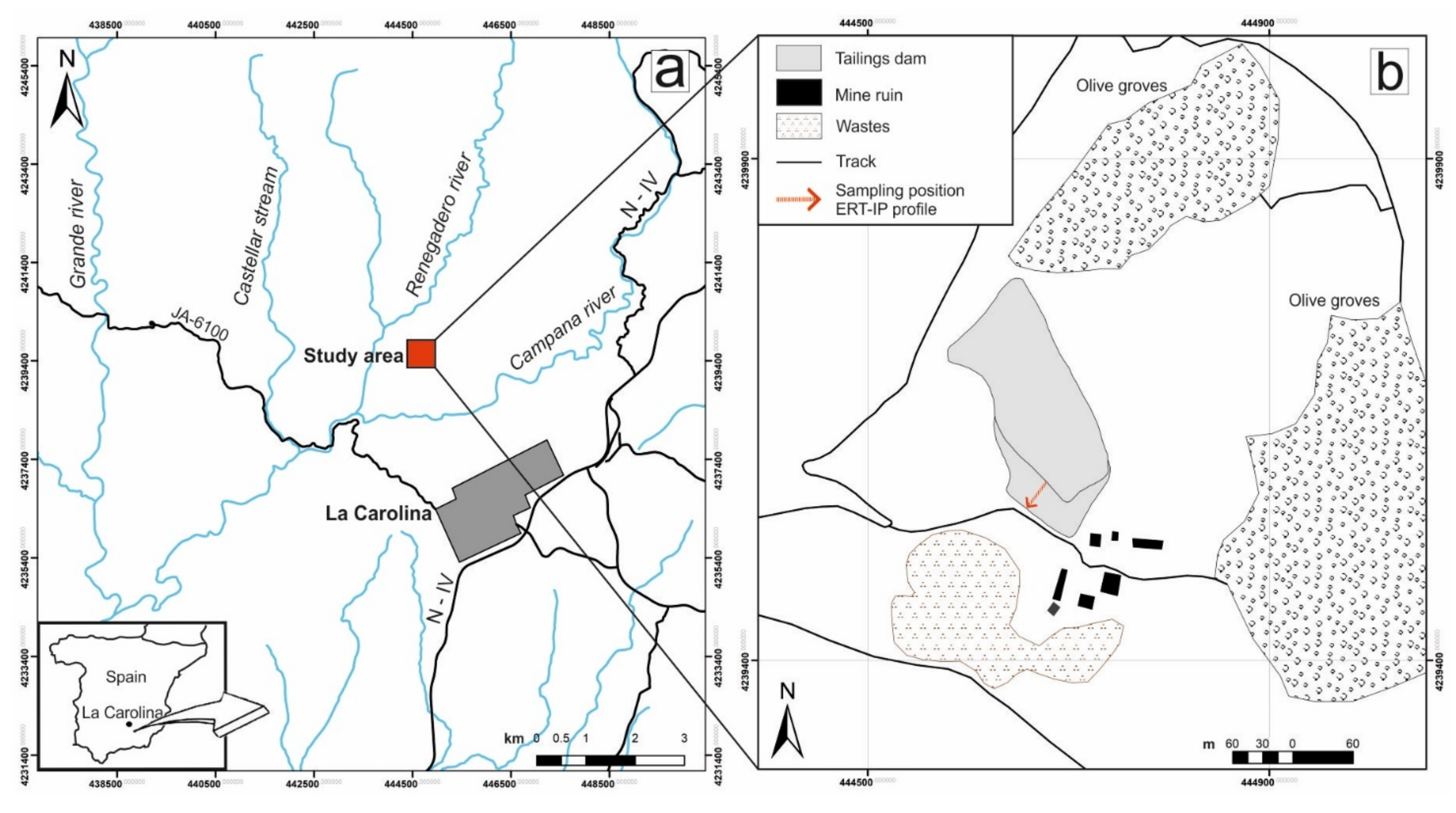
2. Mining in the Study Area

The study area is located on the southeast slope of Sierra Morena within the Hesperian massif (southeast of Spain), where two large geological units stand out at the regional level, consisting of a Palaeozoic basement and a post-Hercynian sedimentary cover [17,18].
The Palaeozoic basement is formed by metamorphic rocks (phyllites with quartzite intercalations), intensely folded during the Hercynian orogeny and subsequently affected by a granitic intrusion. The different tectonic phases generated an extensive network of fractures, which were subsequently filled by a hydrothermal fluid enriched in metallic sulphides, giving rise to the veins deposits of the mining district. The predominant mineralizations in this paragenesis are galena, sphalerite, chalcopyrite, and pyrite, with quartz, ankerite, and calcite as accompanying minerals [19].
Unlike the Palaeozoic basement and fossilizing these mineralizations, the post-Hercynian cover appears to be arranged subhorizontally. It consists of Triassic (red shales and conglomerates), Miocene (marls with layers of sandstones, silts, and/or breccias at the base), and Quaternary materials (silts, sands, and gravels) [20,21].
The mining system used in the district was underground mining using the shrinkage stoping or cut and fill stoping method. It is estimated that the district has approximately 1300 mines, with 65 km of main pits and 786 km of galleries along the vein. This mining district was ranked as the world’s leading producer of lead between 1875 and 1920 [22]. With the ore and host rock obtained from exploitation, comminution and classification operations were carried out as a step prior to the gravimetric concentration process, from which mixed and enriched waste rocks were obtained that were subsequently treated in the flotation process after milling. Through the flotation process, gangue with a particle size of <1 mm with no commercial value was obtained, which was deposited in tailing dams and ponds.
This study was carried out in the vicinity of the Federico Mine, where the dam containing the flotation fines of the concentration process is located (Figure 1b and Figure 2a). This structure lies within a depression in the land where the pumped pulp was retained by a wall composed of the waste rock itself. The waste was deposited without carrying out any previous mitigation efforts to prevent the soils and waters from being affected by the site.

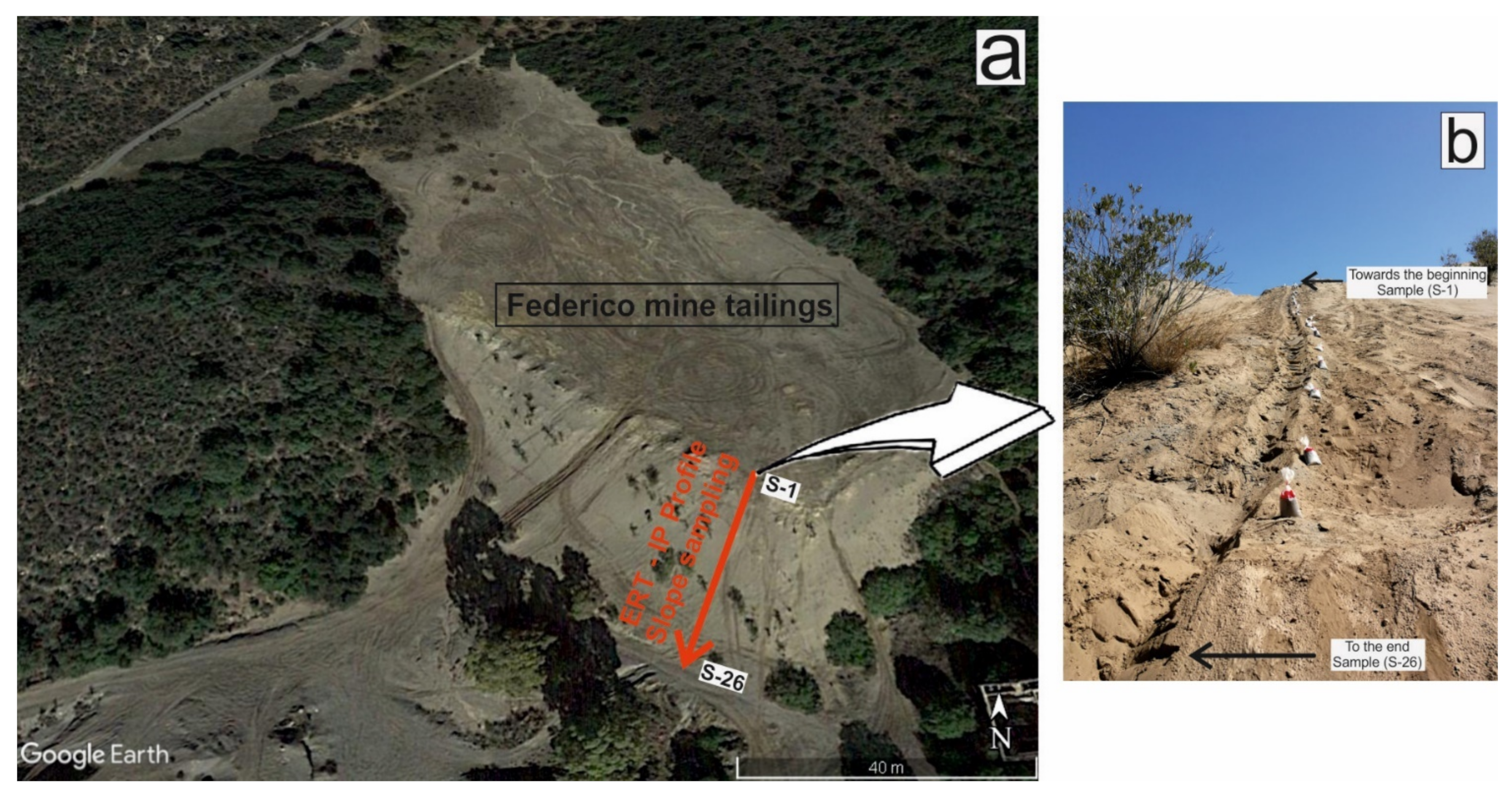
3. Materials and Methods

3.1. Geophysical Techniques

The electrical resistivity tomography (ERT) technique is a noninvasive method that indirectly measures the resistance contributed by a material to the passage of an electric current, obtaining numerical models in the form of 2D profiles or 3D images of the electrical resistivity values [23,24,25,26]. Through automatic data acquisition systems, a large amount of information is obtained that is quickly processed with appropriate software that is able to resolve increasingly complex geological models [27]. In practice, numerous electrodes are placed along a profile, separated according to the degree of resolution and the desired depth [26].
With the induced polarization (IP) method, the electrical charge capacity of a certain body or material in a subsurface is measured; this can identify the materials with the capacity to maintain the current for a given time [23,28]. A known direct current is injected into the ground between two current electrodes and interrupted suddenly to measure the drop in potential between two other potential electrodes. The electrical parameter measured is the apparent chargeability, which corresponds to the area of the voltage decay curve [29,30].
The combination of these two techniques has been used in different areas of earth sciences, such as mining [31,32,33], hydrogeology [34,35], and environmental sciences [8,36,37].
In the flotation fines of the Federico mine dam, ERT and IP surveys were performed to analyse the internal structure of the tailings [38]. For this work, the resistivity and chargeability values obtained in the ERT and IP profiles taken along the slope of the tailing dam were used (Figure 2a). They were obtained using a Wenner–Schlumberger configuration, with a total of 64 electrodes spaced every 0.5 m. The parameters used to measure the resistivity and the chargeability were an 880 V current, time of application = 2000 ms (with a delay of 50 ms) and an interval of 1000 ms (for voltage decay readings), and a Bessel filter and two repetition cycles. The equipment used was a RESECS digital resistivity meter manufactured by Deutsche Montan Technologie (DMT). To generate the resistivity and chargeability values, RES2DINV software was used, which uses the least squares method with forced smoothing and a modified quasi-Newton optimization technique [38].

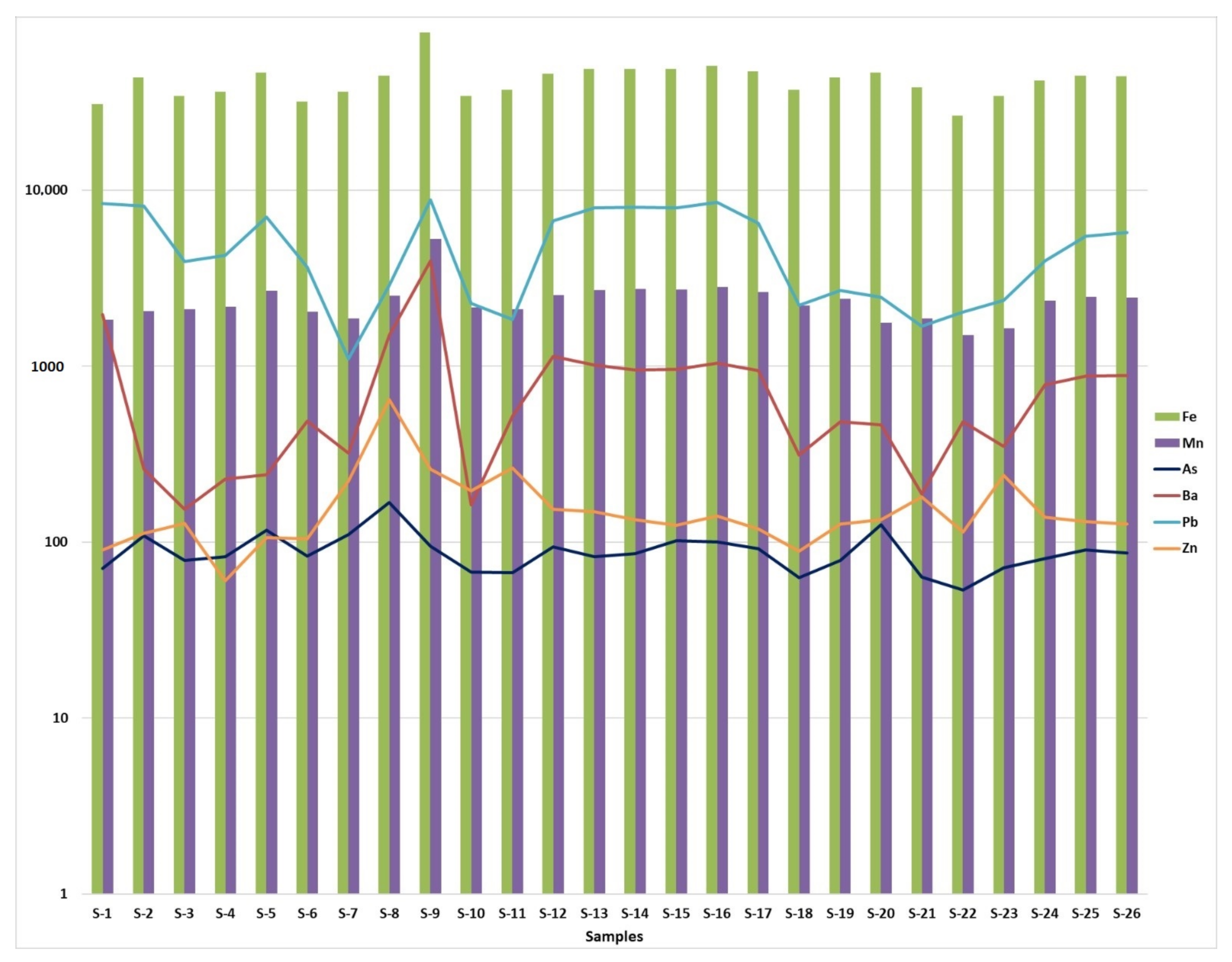
3.2. Geochemical Analysis

A sampling profile was obtained along the slope of the flotation fines dam from the crest to the foot of the slope. In total, 26 sampling points were selected, spaced 1.5 m apart and distributed along a profile 39 m in length (Figure 2b).
Prior to collection of the samples, the surface layer was removed until the unexposed waste was reached (Figure 2b). The sampling criteria adopted were to excavate boreholes 40 cm deep and to take three subsamples at each sampling point. The total amount of each sample obtained was 1.5 to 2 kg, and the samples were stored in plastic bags. Once in the laboratory, after homogenization and air drying for 72 h, the samples were screened using a PVC sieve with a 2-mm mesh. Subsequently, for each sample, the fraction was ground smaller than 2 mm in an agate ball mill Retsch PM 100 model.
For determination of the total metal(loid)s content in the mining waste, the <2-mm fraction was ground in an agate ball mill until a size of less than 50 microns was obtained (Retsch PM 100). Total digestion was carried out by microwave digestion [39] through chemical attack on 0.5 g of the ground sample using HNO3 reagents with addition of H2O2 to facilitate complete oxidation of the organic matter [40].
The analyte obtained by the digestion was analysed by inductively coupled plasma mass spectrometry (ICP–MS) [41]. The analyses were performed at the Centre for Scientific and Technical Instrumentation of the University of Jaen in a mass spectrometer with a plasma torch ionization source and a quadrupole ion filter (model AGILENT 7900).

3.3. Statistical Analysis

Univariate and multivariate statistical techniques were used to determine the interrelationships of and variability in the elements analysed. Data processing was performed using the software SPSS 22 developed by IBM.
The mean, median, range, standard deviation, variance, skewness, and kurtosis were calculated, and histograms, normality plots, and box-and-whisker plots were generated [42].
As a multivariate statistic, a principal component analysis (PCA) of the metal(oid)s present in the slope of the Federico tailing dam was performed. The objective of PCA is to transform a set of original variables into a new set of variables, called factors, that are characterized by being correlated with each other. The first factor or component explains the largest variance of the dataset, the second factor or component explains the second largest variance of the dataset, and so on for the rest of the factors [43,44]. It is interpreted through rotation of the components (axes), with Kaiser–varimax normalization being the most commonly used in geochemistry, which is adequate when the number of components is small. This technique has been used in different environmental scenarios [45,46,47,48].
To combine the geoelectrical and geochemical data, statistical linear regression models were used to evaluate the correlation between the concentration of heavy metals and the values of electrical resistivity and IP. The estimated weighting method was used, which facilitates the calculation of the coefficients of a linear regression model using weighted least squares (WLS). In this way, from the resistivity and chargeability data recorded, the observations that presented greater correlations with the elements analysed received more weight.
As a result, a linear regression model was obtained from the electrical resistivity and chargeability data (Table 1), combined with the concentration of metal(oid)s (Table 2).
Finally, with the mathematical function obtained, the distribution of the lead concentration (mg·kg−1) along the entire slope was calculated. Graphical representation of the results was performed by Surfer 15 software from Golden Software using the kriging method for estimation between the points.

4. Results and Discussion

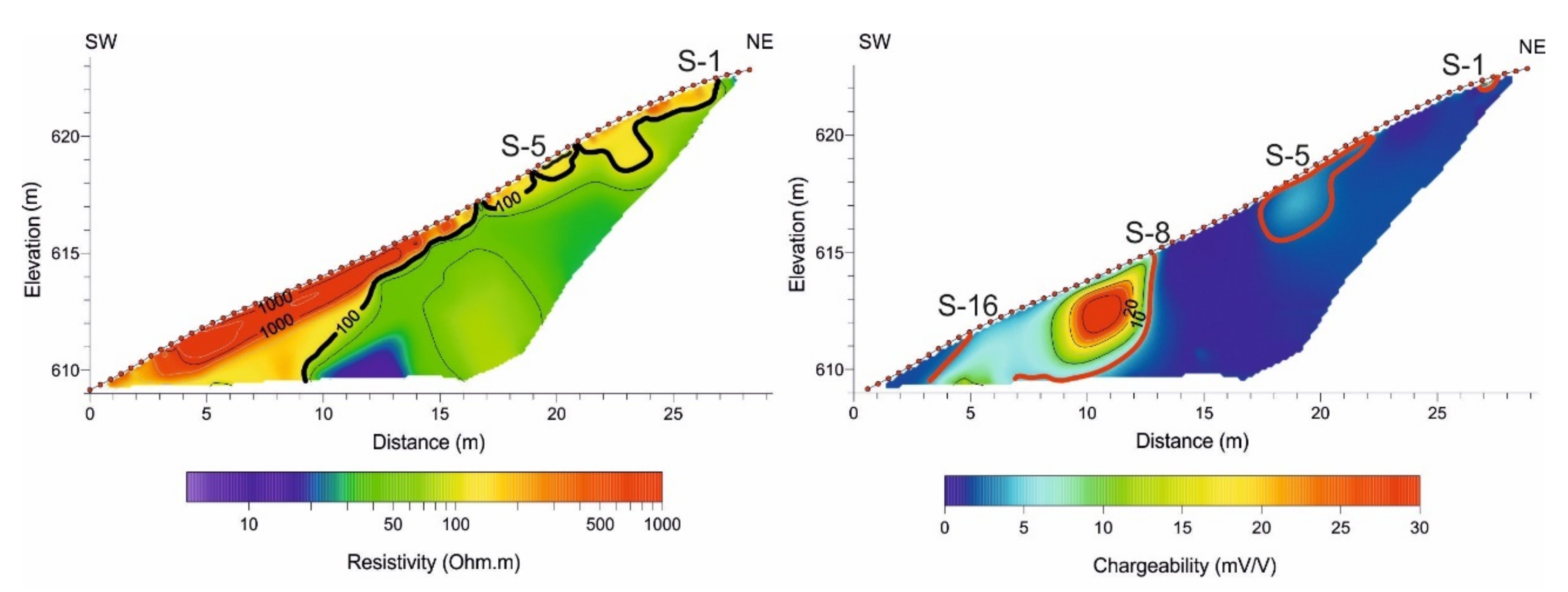
4.1. Resistivity and Chargeability

The geoelectric resistivity and chargeability profiles obtained along the slope of the tailings dam are represented in Figure 3 (modified from [38]). The objective of this geoelectric profile was to obtain an actual resistivity image to verify, as a function of the lateral electrical response obtained, whether the deposited waste was uniform in composition or, on the contrary, if metal(oid)-enriched zones could be differentiated.
As the waste is composed mainly of minerals from the host rocks and, to a lesser extent, of different minerals from the mineral paragenesis of the deposit, it is worth considering that the changes in resistivity and IP recorded are related to the degree of concentration of metal(oid)s in the deposit. To analyse this correlation, the concentration of metals obtained in the samples of fines from the slope was compared with the values of resistivity and chargeability measured at the same points.
Although the maximum depth reached in the resistivity and chargeability profile was 6 m, first, the geophysical data referring to the upper 64 cm of the waste were selected for comparison with the metal (oid) contents obtained from the surface strip of the slope at locations S-1 to S-20 (Figure 2).
According to Samouëlian [49], the variation in electrical resistivity is mainly influenced by the presence of interstitial water and the particle size distribution. Regarding the first factor, note that the degree of moisture present in the waste in the first 64 cm of the profile was very low. On the other hand, the particle size distribution of the deposited waste was uniform, since it came from a concentration plant, where all of the waste was subjected to a series of crushing and milling operations, controlling the particle size by sieving. However, these operations and processes were sometimes difficult to maintain under constant working conditions, which could lead to mineral losses with low recovery. Therefore, the variation in resistivity in the slope is mainly due to the different compositions of the waste. In addition, differences in the concentration of metal(oid)s present in certain areas of the dam would influence the measured chargeability, since electrode polarization occurs when the porous space is blocked by metallic particles [28].
Table 1 includes the actual resistivity and chargeability data used in this work. They correspond to values recorded at the three shallowest depths (12.5 cm, 37.5 cm, and 63.7 cm) for each sampling point. The mean value of the three depths is also presented, which is the value used to calculate the linear regression model.
The concentrations of 15 metal(oid)s (Ag, As, Ba, Ca, Co, Cr, Cu, Fe, Mg, Mn, Ni, P, Pb, V, and Zn) were analysed in the 26 samples taken along the length of the slope. The results obtained are summarized in Table 2. Note the high concentration of Pb obtained; since Pb was the target metal of the concentration process (galena), it should be present at a low concentration in the waste rock, so the high concentration reflects the fact that sometimes, the concentration process was not entirely efficient.
Figure 4 shows the distribution along the slope of six of the metals and semimetals analysed (As, Ba, Fe, Mn, Pb, and Zn). These elements were present in high concentrations and are related to the mineral paragenesis of the study area. The maximum difference obtained between Samples S-8 and S-9 stands out (from 10.5 m to 12 m from the top of the slope), which was observed for all the metal(oid)s analysed. Ba and Pb are present in high amounts with a similar distribution, with these elements presenting the greatest variability among all those analysed. In the case of Pb, abrupt variations are recorded throughout the slope, with high concentrations (above 6000 mg·kg−1) in Samples S-1, S-2, S-5, S-9, S-12, S-13, S-14, S-15, S-16, and S-17, which are located at 0 m, 1.5 m, 6 m, 12 m, 16.5 m, 18 m, 19.5 m, 21 m, 22.5 m and 24 m from the crest of the slope, respectively (Figure 4). The highest concentrations of Ba appear at 0 m and 12 m from the crest of the slope, with a maximum of 3965 mg·kg−1 in Sample S-9.
As, Fe, Mn, and Zn exhibit more homogeneous content distributions. In the case of Fe and Mn, although changes are observed along the slope, they present relatively high values as a whole (with a mean of 42,416 mg·kg−1 of Fe and 2370 mg·kg−1 of Mn), again highlighting the maximum reached in Sample S-9 (78.618 mg·kg−1 for Fe and 5284 mg·kg−1 for Mn). For As and Zn, the concentrations are much more moderate, except in Sample S-8 (at 10.5 m), which presents the maximum values (167 mg·kg−1 of As and 647 mg·kg−1 of Zn; Figure 4).
Figure 3 shows the resistivity and chargeability image obtained from the electrical tomography profile taken on the slope of the Federico dam [38]. The positions of Samples S-1 and S-5 and S-8 to S-16 are also shown, which have the highest contents of metals and semimetals (Figure 4). The positions of these samples coincide with the areas of greatest chargeability and the lowest surface resistivity detected in the profile. The area of maximum surface chargeability values (Figure 3) coincides with samples that present high concentrations of metal(oid)s (S-8 to S-16), especially a high concentration of lead. The surface resistivity obtained in this same section is high, since it is a dry zone whose high chargeability is related to the presence of precipitated salts in the form of metal-rich whitish crusts [38].

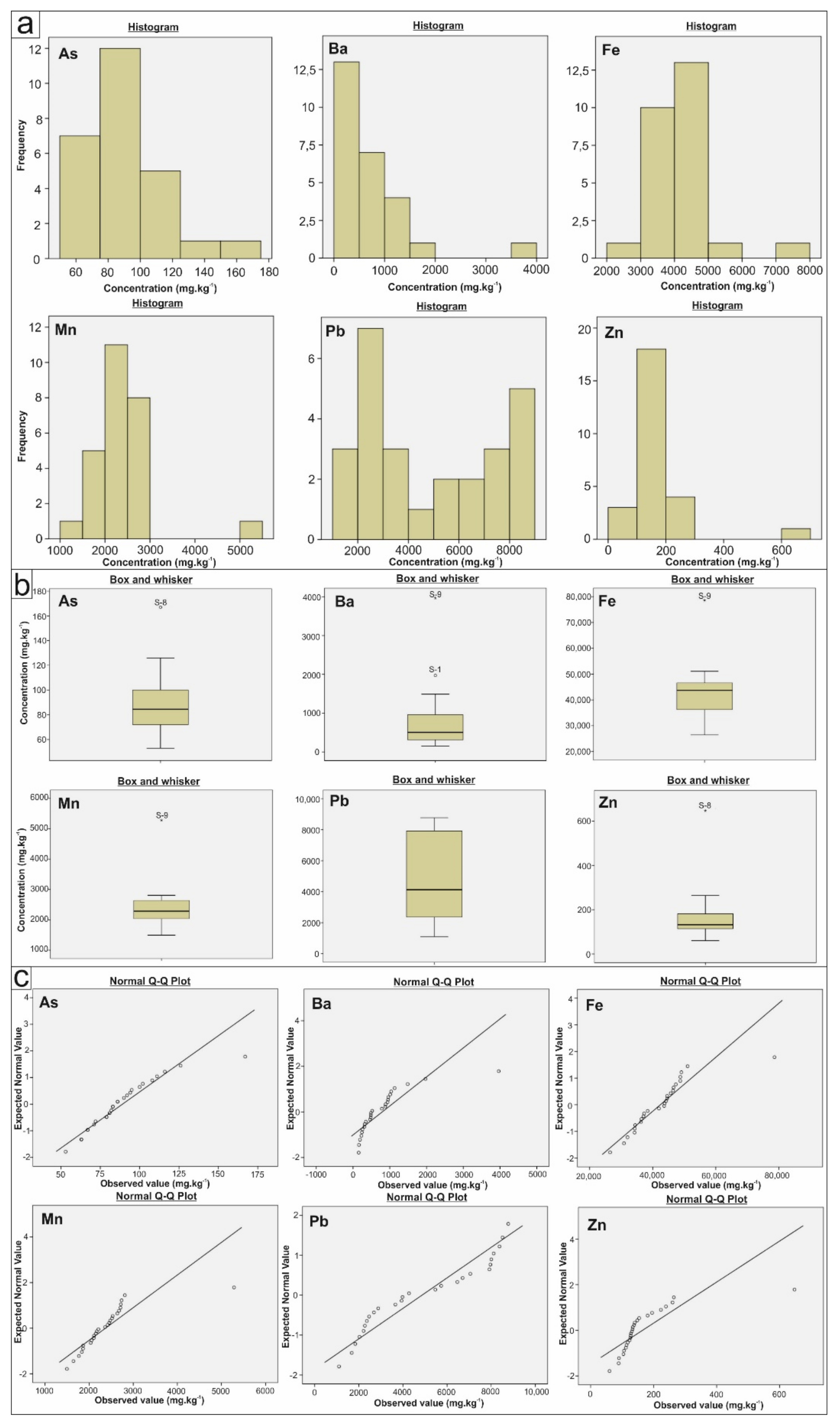
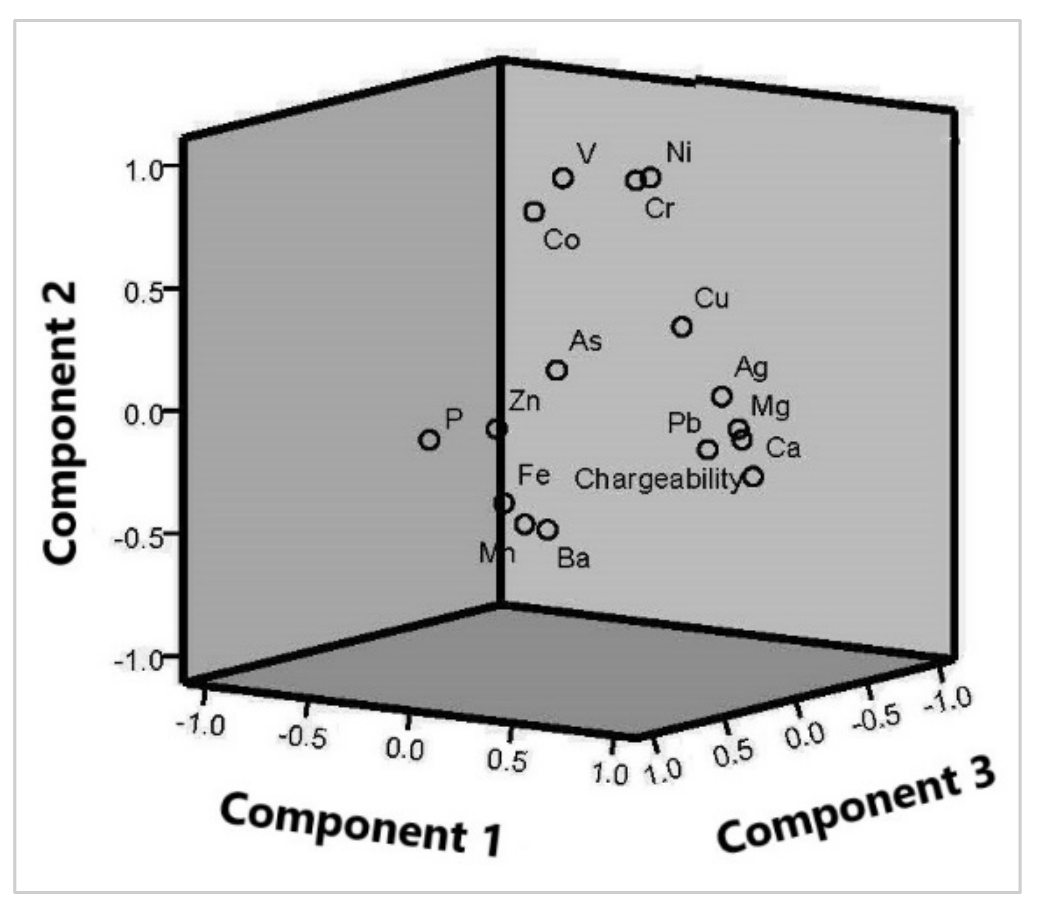
4.2. Univariate and Multivariate Statistics

Table 3 shows the statistical parameters calculated for the six elements that presented high concentrations and that relate to the mineral paragenesis of the study area. The maximum values obtained for As, Ba, Fe, Mn, Pb, and Zn are 167 mg·kg−1, 3965 mg·kg−1, 78,618 mg·kg−1, 5284 mg·kg−1, 8772 mg·kg−1, and 647 mg·kg−1, respectively. In the case of Ba, Pb, and Zn, there is a greater difference between the mean and the median obtained, presenting a wide range of variation (Table 3).
In all cases, except for As, the standard deviation and variance are characterized by high values, indicating that most samples have values far from their mean.
As, Ba, Fe, Mn, and Zn have a greater number of values below the mean than above it, but in any case, the concentrated values close to the mean are high and present a positive asymmetry and kurtosis. Pb has the lowest concentration of values around its mean; that is, its values lie furthest from the mean and are predominantly located close to the minimum and maximum values (Table 3).
All the histograms obtained (Figure 5a) group the majority of samples for each element off-centre with asymmetry to the right, with the exception of Pb, which has two maximums at the extremes, with the mean concentration being the least frequent.
The box-and-whisker plots (Figure 5b) show off-centred medians for Ba, Fe, Mn, Pb, and Zn, with the exception of As. Note the wide box of Pb, which indicates the large range of Pb content throughout the entire slope. For the rest of the elements, especially Mn and Zn, the amplitude of the box is reduced due to a closer quartile 1 and quartile 3. Values considered atypical are identified in Sample S-8 for As and Zn; in S-9 for Ba, Fe, and Mn; and in S-1 for Ba. As mentioned before, these are the samples in which the maximum concentrations were identified.
The values of the contents of As, Fe, and Mn present a normal distribution. The same does not happen in the case of Ba, Pb, and Zn, which present a lognormal distribution (Figure 5c). In addition, Ba and Zn present a distribution of values very far from normal due to Samples S-8 and S-9.
A multivariate statistical analysis was performed using PCA, and the original number of variables was reduced to a smaller number of variables. These principal components (PCs) are able to explain a large part of the total variability; in this case, the four PCs obtained represent 80% of the total variance. In addition, the component graph is shown in rotated three-dimensional space (Figure 6).
The first PC (Table 4), which represents the maximum variance, is composed of Ag, Ca, Cu, chargeability, Mg, and Pb. Ag, Cu, and Pb are the metals associated with the mineral paragenesis in the mining basin of the study area. Ca and Mg also contribute, since they are elements associated with the carbonate minerals that accompany the mineralization of galena. The association of chargeability with these metal(oid)s indicates that their variability is mainly due to the concentration of these elements.
Co, Cr, Ni, and V were found as elements of the second PC (Table 4). This association is related to the country rock, consisting of phyllites, which justifies the low values obtained in the flotation sludge. In the case of Ni, the concentration that appeared in the river sediments of this drainage basin was greater than that obtained in the Federico tailing dam [6].
In the third PC (Table 4), Ba, Fe, and Mn are associated. These three metals are related to the mineral paragenesis of the mining basin and are usually associated with some of the mined minerals.
Finally, the fourth PC (Table 4) has the lowest representation of the total variance. In this component, we find As and Zn, which are frequent elements in the study area because they are associated with mineralization. However, as with Ni, its concentrations are lower in this deposit of mining waste than those found in the sediments of the water channels.
Figure 6 shows the grouping of the different variables in a space rotated in three dimensions (components), which represents 68% of the variance. In this way, we can see the position of each variable influenced by the three PCs. The associations produced are the same as those obtained in the rotated matrix (Table 4). For Component 1, the most saturated variables are Ag, Ca, Cu, chargeability, Mg, and Pb, with Ca and Mg superimposed. In the case of Component 2, they are Co, V, Cr, and Ni. Finally, Component 3 is formed by Ba, Fe, and Mn.
The different legislations on contaminated soils establish allowable generic reference levels (GRLs), where there are possible impacts on humans and/or ecosystems if the levels are exceeded. In this work, both the GRLs established in the regulation concerning contaminated soils in Andalusia [50] and the levels included in the Dutch regulations [51], some of the most internationally applied levels in the study of soils affected by mining [52,53], were considered.
Table 3 highlights the values that exceed the limit set by the Andalusian regional regulations in bold and those that exceed the maximum allowable concentrations established by the Dutch standard in grey.
The mean concentrations of As and Pb exceed the reference values for contaminated soils in both the Andalusian and Dutch regulations. In the case of As, even the minimum concentration obtained exceeds the value of the regional regulations, which are more restrictive than the Dutch equivalents for this element. Additionally, the mean content of Ba presents values that exceed the limit established by the Dutch regulations. However, the Pb content of these mining wastes stand out, since in all the samples analysed, there are concentrations that far exceed the reference values of the two regulations considered.

4.3. Estimation of the Pb Content

Of all the metal(oid)s analysed, the distribution of lead inside the flotation dam was analysed. Given its potentially toxic nature and the high concentrations existing in the upper strip of the studied slope, the distribution of this metal inside the mining dam is of interest.
Both the chargeability and the resistivity are influenced by the metal(oid) content, but the chargeability has a stronger relationship with the metals. Therefore, after the chargeability–Pb affinity was verified by PCA, a weighted linear regression was used, with the weighting variable being the chargeability, which allowed the calculation of the coefficients of a linear regression model using WLS so that more accurate observations were given greater weight. For the calculation, resistivity and chargeability were taken as independent variables, taking the mean values along the slope (Table 1). The dependent variable was Pb, taking the concentration values from Samples S-1 to S-20 (Table 2).
The equation obtained from the linear regression model with weighted estimation is:
PE (Pb) = (4.2 × Res.) + (547 × Charg.)
where PE (Pb) is the weighted estimate of the lead concentration (in mg·kg−1), Res. is the actual electrical resistivity (expressed in Ohm m), and Charg. is the chargeability (expressed in mV·V−1). For this equation, the power used in the weighting is −0.5, since this power has the lowest logarithmic value of likelihood.
The linearity between the dependent variable and the independent variables is significant, since they have a correlation coefficient (R) of 0.9 and a coefficient of determination (R2) of 0.8. The residual values were verified to be independent according to the Durbin–Watson factor, which presented a value of 1.7. In the collinearity diagnosis, the value obtained for the inflation factors of the variance of each of the predictor variables was 1.3, which justified the noncollinearity between the independent variables; that is, there is no correlation between them.
Equation (1) was used to estimate the Pb content from the 342 resistivity and chargeability data recorded for the inside slope (Figure 3). The results obtained for the weighted estimation of the Pb content are graphically represented in Figure 7, where the image of the lead concentration along the slope profile is shown. Three ranges are differentiated for the distribution of Pb content. The first range corresponds to values lower than 4000 mg·kg−1 (the mean value of the Pb content of the sampling profile), the second ranges from 4000 to 6000 mg·kg−1, and the third corresponds to values greater than 6000 mg·kg−1. The minimum value of lead in the profile is above 1000 mg·kg−1, which exceeds the limit established by the regional (275 mg·kg−1) and Dutch regulations (530 mg·kg−1). Estimated maximums above 14,000 mg·kg−1 can be observed in the lower zone of the slope. In addition, in this medium-lower zone of the dam, there are other areas with values above 8000 mg·kg−1, which exceeds the maximum concentration obtained in the surface samples. This medium-lower zone coincides with a greater presence of whitish precipitate crusts [38], characterized by a high metallic content.

5. Conclusions

Sampling was carried out along a cut made in the slope of a tailing dam of flotation fines, and the metal(oid)s of these mining wastes were analysed. Of the 15 elements analysed, As, Ba, Fe, Mn, Pb, and Zn were selected as the most significant, either because of their contents or because of their relationship with mineral paragenesis. The highest concentrations appeared in the lower third of the slope between sampling points S-8 and S-9, associated with high values of chargeability.
The histograms, box-and-whisker plots, and Q-Q plots indicated that the contents of As, Fe, and Mn presented normal behaviour, except for the presence of some extreme values. However, Ba, Pb, and Zn showed lognormal behaviour.
The multivariate analysis performed using PCA extracted four components that explained 80% of the total variance. The first component grouped Ag, Ca, chargeability, Cu, Mg, and Pb, where Ag, Cu, and Pb are the main paragenetic metals, while Ca and Mg are the ones mainly accompanying mineralization. The second component included Co, Cr, Ni, and V, which are linked to the host rock, consisting of Palaeozoic phyllites. In the third component, Ba, Fe, and Mn were associated; these are also related to paragenesis minerals. Finally, the fourth group contained As and Zn, elements related to mineralization.
Pb is the most characteristic element of this paragenesis and the most abundant metal in the waste, and is considered potentially toxic according to current regulations. All the values obtained for the concentration of Pb in the samples of the slope of the Federico dam exceed the limits established by environmental regulations, both regional and European.
Using the linear regression model with estimated weighting, the distribution of Pb inside the tailing dam was obtained. For this, the resistivity and chargeability values of the terrain were correlated with the geochemical data obtained from the surface samples. However, in this work, estimation of the distribution of metals within the residue was carried out by estimating the weighting of the chargeability variable, a variable obtained by the induced polarization (IP) method.
The model determines the variation in the distribution of the Pb content with depth without the need to apply direct techniques (mechanical drilling). The combination of geophysical, geochemical, and statistical tools constitutes an acceptable and low-cost methodology compared with other methodologies used to estimate the distribution of metal(oid) contents inside mining dams. This mining district has another 32 mining dams with a volume of approximately 10,500,000 m3; in these dams, the concentration of chemical elements is similar to that in this mining dam. Therefore, the application of this methodology would be very useful to transform these environmental liabilities into mining, environmental, or social assets.

Author Contributions

Conceptualization, R.M., J.M. and M.C.H.; Formal analysis, J.M. and M.C.H.; Investigation, R.M. and M.J.C.-S.; Methodology, R.M., J.M. and M.J.C.-S.; Resources, R.M. and M.J.C.-S.; Software, R.M.; Supervision, J.M., M.C.H. and M.J.C.-S.; Validation, J.M. and M.C.H.; Visualization, R.M.; Writing—original draft, R.M.; Writing—review & editing, R.M., J.M. and M.C.H. All authors have read and agreed to the published version of the manuscript.

Funding

This research was funded by the project FEDER 2020, Grant Number 1380520.

Conflicts of Interest

The authors declare no conflict of interest.

References

  1. Edraki, M.; Baumgartl, T.; Manlapig, E.; Bradshaw, D.; Franks, D.M.; Moran, C.J. Designing mine tailings for better environmental, social and economic outcomes: A review of alternative approaches. J. Clean. Prod. 2014, 84, 411–420. [Google Scholar] [CrossRef]
  2. Byrne, P.; Reid, I.; Wood, P.J. Sediment geochemistry of streams draining abandoned lead/ zinc mines in central Wales: The Afon Twymyn. J. Soils Sediments 2010, 10, 683–697. [Google Scholar] [CrossRef] [Green Version]
  3. Resongles, E.; Casiot, C.; Freydier, R.; Dezileau, L.; Viers, J.Ô.; Elbaz-Poulichet, F. Persisting impact of historical mining activity to metal (Pb, Zn, Cd, Tl, Hg) and metalloid (As, Sb) enrichment in sediments of the Gardon River, Southern France. Sci. Total Environ. 2014, 481, 509–521. [Google Scholar] [CrossRef] [PubMed]
  4. Ciszewski, D. The past and prognosis of mining cessation impact on river sediment pollution. J. Soils Sediments 2019, 19, 393–402. [Google Scholar] [CrossRef] [Green Version]
  5. Cortada, U.; Hidalgo, M.; Martínez, J.; Rey, J. Dispersion of metal(loid)s in fluvial sediments: An example from the Linares mining district (southern Spain). Int. J. Environ. Sci. Technol. 2019, 16, 469–484. [Google Scholar] [CrossRef]
  6. Mendoza, R.; Martínez, J.; Rey, J.; Hidalgo, M.; Campos, M. Metal(loid)s Transport in Hydrographic Networks of Mining Basins: The Case of the La Carolina Mining District (Southeast Spain). Geosciences 2020, 10, 391. [Google Scholar] [CrossRef]
  7. Hudson-Edwards, K.A.; Macklin, M.G.; Brewer, P.A.; Dennis, I.A. Assessment of Metal Mining-Contaminated River. 2008. Available online: http://www.eugris.info/displayresource.aspx?r=6681 (accessed on 10 June 2020).
  8. Lghoul, M.; Teixidó, T.; Peña, J.A.; Hakkou, R.; Kchikach, A.; Guerin, R.; Jaffal, M.; Zouhri, L. Electrical and Seismic Tomography Used to Image the Structure of a Tailings Pond at the Abandoned Kettara Mine, Morocco. Mine Water Environ. 2012, 31, 53–61. [Google Scholar] [CrossRef]
  9. Placencia-Gómez, E.; Parviainen, A.; Hokkanen, T.; Loukola-Ruskeeniemi, K. Integrated geophysical and geochemical study on AMD generation at the Haveri Au–Cu mine tailings, SW Finland. Environ. Earth Sci. 2010, 61, 1435–1447. [Google Scholar] [CrossRef]
  10. Martínez, J.; Hidalgo, M.; Rey, J.; Garrido, J.; Kohfahl, C.; Benavente, J.; Rojas, D. A multidisciplinary characterization of a tailings pond in the Linares-La Carolina mining district, Spain. J. Geochem. Explor. 2016, 162, 62–71. [Google Scholar] [CrossRef]
  11. Ceniceros-Gómez, A.E.; Macías-Macías, K.Y.; de la Cruz-Moreno, J.E.; Gutiérrez-Ruiz, M.E.; Martínez-Jardines, L.G. Characterization of mining tailings in México for the possible recovery of strategic elements. J. South Am. Earth Sci. 2018, 88, 72–79. [Google Scholar] [CrossRef]
  12. Cortada, U.; Hidalgo, M.; Martínez, J.; Rey, J. Impact in soils caused by metal(loid)s in lead metallurgy. The case of La Cruz Smelter (Southern Spain). J. Geochem. Explor. 2018, 190, 302–313. [Google Scholar] [CrossRef]
  13. Martínez, J.; Rey, J.; Hidalgo, M.; Garrido, J.; Rojas, D. Influence of measurement conditions on the resolution of electrical resistivity imaging: The example of abandoned mining dams in the la Carolina District (Southern Spain). Int. J. Miner. Process. 2014, 133, 67–72. [Google Scholar] [CrossRef]
  14. Cortada, U.; Martínez, J.; Rey, J.; Hidalgo, M.; Sandoval, S. Assessment of tailings pond seals using geophysical and hydrochemical techniques. Eng. Geol. 2017, 223, 59–70. [Google Scholar] [CrossRef]
  15. Rojas, D.; Hidalgo, M.; Kohfahl, C.; Rey, J.; Martínez, J.; Benavente, J. Oxidation Dynamics and Composition of the Flotation Plant Derived Tailing Impoundment Aquisgrana (Spain). Water Air Soil Pollut. 2019, 230, 158. [Google Scholar] [CrossRef]
  16. IGME. Inventario Nacional de Depósitos de Lodos. 2002. Available online: http://info.igme.es/catalogo/resource.aspx?portal=1&catalog=3&ctt=1&lang=por&dlang=eng&llt=dropdown&master=infoigme&shdt=false&shfo=false&resource=18 (accessed on 13 August 2021).
  17. Tamain, G. Recherches Géologiques et Minières en Sierra Morena Orientale (Espagne); Laboratoire de Géologie Structurale et Appliquée: Paris, France, 1972. [Google Scholar]
  18. Castelló, R.; Orviz, F. Mapa Geológico y Memoria Explicativa de la Hoja 884 (La Carolina), Escala 1:50.000. 1976. Available online: http://info.igme.es/cartografiadigital/geologica/Magna50.aspx (accessed on 13 August 2021).
  19. Lillo, F.J. Geology and Geochemistry of Linares—La Carolina Pb-ore Field (Sootheastern Border of the Hesperian Massif). 1992. Available online: https://etheses.whiterose.ac.uk/12721/ (accessed on 13 August 2021).
  20. Rey, J.; Hidalgo, M.; Martínez, J. Upper Ordovician–Lower Silurian transgressive–regressive cycles of the Central Iberian Zone (NE Jaén, Spain). Geol. J. 2005, 40, 477–495. [Google Scholar] [CrossRef]
  21. Azcárate, J.E. Mapa Geológico y Memoria Explicativa de la Hoja 905 (Linares), Escala 1:50.000; Instituto Geológico y Minero de España: Madrid, Spain, 1977. [Google Scholar]
  22. Junta de Andalucía. Libro Blanco de la Minería Andaluza; Junta de Andalucía: Seville, Spain, 1986; Volume 2. [Google Scholar]
  23. Telford, W.M.; Geldart, L.P.; Sheriff, R.E. Applied Geophysics, 2nd ed.; Cambridge University Press: Cambridge, UK, 1990. [Google Scholar] [CrossRef]
  24. Store, H.; Storz, W.; Jacobs, F. Electrical Resistivity Tomography to Investigate Geological Structures of Earth’s Upper Crust. Geophys. Prospect. 2000, 48, 455–471. [Google Scholar] [CrossRef]
  25. Dahlin, T.; Zhou, B. A numerical comparison of 2D resistivity imaging with 10 electrode arrays. Geophys. Prospect. 2004, 52, 379–398. [Google Scholar] [CrossRef] [Green Version]
  26. Sasaki, Y. Resolution of Resistivity Tomography Inferred from Numerical Simulation. Geophys. Prospect. 1992, 40, 453–463. [Google Scholar] [CrossRef]
  27. Griffiths, D.; Barker, R. Two-dimensional resistivity imaging and modeling in areas of complex geology. J. Appl. Geophys. 1993, 29, 211–226. [Google Scholar] [CrossRef]
  28. Summer, J.S. Principles of Induced Polarization for Geophysical Exploration; Developments in Economic Geology; Elsevier: Amsterdam, The Netherlands, 1976; Volume 5. [Google Scholar]
  29. Zhdanov, M. Chapter 12—Direct Current and Induced Polarization Methods. In Foundations of Geophysical Electromagnetic Theory and Methods, 2nd ed.; Zhdanov, M.S., Ed.; Elsevier: Amsterdam, The Netherlands, 2018; pp. 439–493. [Google Scholar]
  30. Vinegar, H.J.; Waxman, M.H. Induced polarization of shaly sands. Geophysics 1984, 49, 1267–1287. [Google Scholar] [CrossRef]
  31. Mostafaei, K.; Ramazi, H. Compiling and verifying 3D models of 2D induced polarization and resistivity data by geostatistical methods. Acta Geophys. 2018, 66, 959–971. [Google Scholar] [CrossRef]
  32. Heritana A, R.; Riva, R.; Ralay, R.; Boni, R. Evaluation of flake graphite ore using self-potential (SP), electrical resistivity tomography (ERT) and induced polarization (IP) methods in east coast of Madagascar. J. Appl. Geophys. 2019, 169, 134–141. [Google Scholar] [CrossRef]
  33. Martínez, J.; Rey, J.; Sandoval, S.; Hidalgo, M.; Mendoza, R. Geophysical Prospecting Using ERT and IP Techniques to Locate Galena Veins. Remote Sens. 2019, 11, 2923. [Google Scholar] [CrossRef] [Green Version]
  34. Revil, A.; Karaoulis, M.; Johnson, T.; Kemna, A. Review: Some low-frequency electrical methods for subsurface characterization and monitoring in hydrogeology. Hydrogeol. J. 2012, 20, 617–658. [Google Scholar] [CrossRef]
  35. Chirindja, F.J.; Dahlin, T.; Juizo, D.; Steinbruch, F. Reconstructing the formation of a costal aquifer in Nampula province, Mozambique, from ERT and IP methods for water prospection. Environ. Earth Sci. 2017, 76, 36. [Google Scholar] [CrossRef] [Green Version]
  36. Zarroca, M.; Linares, R.; Velásquez-López, P.C.; Roqué, C.; Rodríguez, R. Application of electrical resistivity imaging (ERI) to a tailings dam project for artisanal and small-scale gold mining in Zaruma-Portovelo, Ecuador. J. Appl. Geophys. 2015, 113, 103–113. [Google Scholar] [CrossRef]
  37. Rey, J.; Martínez, J.; Hidalgo, M.; Mendoza, R.; Sandoval, S. Assessment of Tailings Ponds by a Combination of Electrical (ERT and IP) and Hydrochemical Techniques (Linares, Southern Spain). Mine Water Environ. 2020, 40, 298–307. [Google Scholar] [CrossRef]
  38. Martínez, J.; Mendoza, R.; Rey, J.; Sandoval, S.; Hidalgo, M.C. Characterization of Tailings Dams by Electrical Geophysical Methods (ERT, IP): Federico Mine (La Carolina, Southeastern Spain). Minerals 2021, 11, 145. [Google Scholar] [CrossRef]
  39. Langston, W.J.; Spence, S.K. Metal Analysis. A Handbook of ecotoxicology. Volume 2; Blackwell Sci.: London, UK, 1994. [Google Scholar]
  40. Xing, B.; Veneman, P.L.M. Microwave digestion for analysis of metals in soil. Commun. Soil Sci. Plant Anal. 1998, 29, 923–930. [Google Scholar] [CrossRef]
  41. U.S. EPA. Method 200.8: Determination of Trace Elements in Waters and Wastes by Inductively Coupled Plasma-Mass Spectrometry; U.S. EPA: Cincinnati, OH, USA, 1994; Revision 5.4. [Google Scholar]
  42. Zhang, C.; Selinus, O. Statistics and GIS in environmental geochemistry—Some problems and solutions. J. Geochem. Explor. 1998, 64 Pt 1, 339–354. [Google Scholar] [CrossRef]
  43. Einax, J.W.; Truckenbrodt, D.; Kampe, O. River Pollution Data Interpreted by Means of Chemometric Methods. Microchem. J. 1998, 58, 315–324. [Google Scholar] [CrossRef]
  44. Lee, C.S.; Li, X.; Shi, W.; Cheung, S.C.; Thornton, I. Metal contamination in urban, suburban, and country park soils of Hong Kong: A study based on GIS and multivariate statistics. Sci. Total Environ. 2006, 356, 45–61. [Google Scholar] [CrossRef] [Green Version]
  45. Anju, M.; Banerjee, D.K. Multivariate statistical analysis of heavy metals in soils of a Pb–Zn mining area, India. Environ. Monit. Assess. 2012, 184, 4191–4206. [Google Scholar] [CrossRef] [PubMed]
  46. Astel, A.; Tsakovski, S.; Barbieri, P.; Simeonov, V. Comparison of self-organizing maps classification approach with cluster and principal components analysis for large environmental data sets. Water Res. 2007, 41, 4566–4578. [Google Scholar] [CrossRef] [PubMed]
  47. Lu, X.; Wang, L.; Li, L.Y.; Lei, K.; Huang, L.; Kang, D. Multivariate statistical analysis of heavy metals in street dust of Baoji, NW China. J. Hazard. Mater. 2010, 173, 744–749. [Google Scholar] [CrossRef] [PubMed]
  48. Tahri, M.; Bounakhla, M.; Bilal, E.; Gruffat, J.J.; Moutte, J.; Garcia, D. Multivariate analysis of heavy metal contents in soils, sediments and water in the region of Meknes (Central Morocco). Environ. Monit. Assess. 2005, 102, 405–417. [Google Scholar] [CrossRef] [PubMed]
  49. Samouëlian, A.; Cousin, I.; Tabbagh, A.; Bruand, A.; Richard, G. Electrical resistivity survey in soil science: A review. Soil Tillage Res. 2005, 83, 173–193. [Google Scholar] [CrossRef] [Green Version]
  50. Real Decreto 18/2015. de 27 de Enero. Boletín Oficial de la Junta de Andalucía. Consejería de Medio Ambiente y Ordenación del Territorio. Consejería de Medio Ambiente y Ordenación del Territorio, Vol. Núm. 38. Junta de Andalucía. Available online: https://www.juntadeandalucia.es/boja/2015/38/3 (accessed on 13 August 2021).
  51. Rijkswaterstaat. Soil Remediation Circular Version of 1 July 2013. 2013. Available online: https://rwsenvironment.eu/subjects/soil/legislation-and/soil-remediation/ (accessed on 13 August 2021).
  52. Esquenazi, E.L.; Norambuena, B.K.; Bacigalupo, Í.M.; Estay, M.G. Evaluation of soil intervention values in mine tailings in northern Chile. PeerJ 2018, 2018, e5879. [Google Scholar] [CrossRef] [PubMed]
  53. Kyere, V.N.; Greve, K.; Atiemo, S.M.; Amoako, D.; Aboh, I.K.; Cheabu, B.S. Contamination and Health Risk Assessment of Exposure to Heavy Metals in Soils from Informal E-Waste Recycling Site in Ghana. Emerg. Sci. J. 2018, 2, 428. [Google Scholar] [CrossRef]
Figure 1. (a) Georeferenced location of the study area (ETRS89/UTM zone 30N). (b) Location of the tailing dam in the Federico mine, indicating the position along the slope of the ERT-IP profile.
Minerals 12 00007 g001
Figure 2. (a) Orthophoto of the tailing dam. The location of the ERT-IP profile and sampling location in the tailings is indicated. (b) Sampling points on the slope of the dam and the position of the samples S-1 (top) and S-26 (bottom).
Minerals 12 00007 g002
Figure 3. Image of the actual electrical resistivity (Ohm m) and chargeability (mV·V−1) of the ERT-IP profile along the slope of the dam (modified from [38]). The position of the samples of fines with the highest concentration of metals is indicated.
Minerals 12 00007 g003
Figure 4. Distribution of the concentrations (expressed in logarithmic scale in base 10) of As, Ba, Fe, Mn, Pb, and Zn along the slope of the tailing dam.
Minerals 12 00007 g004
Figure 5. Univariate statistics: (a) histograms, (b) box-and-whisker plots, and (c) normal Q-Q plots for the concentration of metals along the slope of the tailing dam.
Minerals 12 00007 g005
Figure 6. Rotation of PCs using the varimax procedure.
Minerals 12 00007 g006
Figure 7. Image of the lead distribution in the profile studied along the slope of the tailing dam. The position of the samples with the highest metal concentration is indicated.
Minerals 12 00007 g007
Table 1. Electrical resistivity and chargeability values measured at depths of 12.5 cm, 37.5 cm, and 63.7 cm along the slope of the Federico mine dam.
Resistivity (Ohm.m)Chargeability (mV/V)
PositionDepth: 12.5 cmDepth: 37.5 cmDepth: 63.7 cmMeanDepth: 12.5 cmDepth: 37.5 cmDepth: 63.7 cmMean
S-1 (0.0 m)225.4092.2236.17117.9316.6013.909.4713.32
S-2 (1.5 m)189.64177.48147.60171.571.881.781.491.72
S-3 (3.0 m)289.71217.29104.23203.740.700.800.910.80
S-4 (4.5 m)240.92182.55139.80187.760.840.650.400.63
S-5 (6.0 m)158.76141.98114.94138.564.654.494.194.44
S-6 (7.5 m)62.9780.6687.8777.175.985.184.495.22
S-7 (9.0 m)140.21131.2589.45120.303.693.203.023.30
S-8 (10.5 m)145.02144.13123.37137.510.310.320.330.32
S-9 (12.0 m)171.50166.30120.02152.610.040.090.160.10
S-10 (13.5 m)290.95247.12139.20225.769.288.046.738.02
S-11 (15.0 m)1073.30860.20536.88823.460.490.290.180.32
S-12 (16.5 m)1021.801288.701168.701159.732.721.580.741.68
S-13 (18.0 m)975.411227.701705.201302.774.714.493.634.28
S-14 (19.5 m)817.221158.901871.701282.613.383.042.352.92
S-15 (21.0 m)952.911157.201809.001306.378.857.575.867.43
S-16 (22.5 m)845.771204.601775.401275.262.452.372.002.27
S-17 (24.0 m)1576.202258.003485.402439.870.070.080.080.08
S-18 (25.5 m)1788.002268.202847.102301.100.010.010.000.01
S-19 (27.5 m)250.50282.27314.34282.370.830.760.670.75
S-20 (29.0 m)281.96251.90150.55228.141.391.491.631.50
Table 2. The concentration (mg·kg−1) of metal(oid)s in the samples of fines from the slope of the Federico mine dam.
SampleAgAsBaCaCoCrCuFeMgMnNiPPbVZn
S-16.171197226,3116111030,88510,2151834164348375890
S-26.010825824,7418121243,76510,67720551952181109112
S-32.77915423,3277161034,31410,265210617489393911128
S-42.88322825,779612536,26310,9292171154524273860
S-54.711624135,022791146,46216,04826771939070517106
S-64.18348719,9351117631,995903020352342636569104
S-71.411131916,8701018836,4218461186323505110111223
S-82.4167148821,225891244,5799753251817536287810647
S-95.095396527,25563778,61812,22052841045287725260
S-101.26716221,63674534,425848221541356822746195
S-111.36752114,66576637,266595721111455218378264
S-124.994113320,212815945,7079608253419437670311154
S-135.982101021,9228121048,74710,96227102043979179148
S-145.88695222,2558121048,72211,27527361943080039133
S-155.610296022,1888121049,08210,99527182044479629124
S-165.6100103822,1948121451,07211,41028092044785149140
S-174.69294220,904713947,33610,380263819443646310118
S-182.06331217,427712937,07482062210184682213989
S-192.47948216,931811943,618807824201949626839126
S-201.4126462864984746,616360317671358524668134
S-211.36318811,80265738,404419818621160016798181
S-221.25348515,58945726,461645614961052920306114
S-231.57235013,337751034,235549416431458723627239
S-243.38178518,2528101141,967848023611750339799138
S-254.59087719,103891244,565916424761748154678131
S-264.48688518,886710944,230911124551746957329127
Table 3. Descriptive statistics of the total concentration of metal(oid)s. Values above the generic reference levels defined by the Andalusian government for contaminated soils are highlighted in bold. The shaded values are those that exceed the intervention values established by the Dutch regulations.
Element(mg·kg−1)VarianceSkewnessKurtosis
Min.Max.MeanMedianRangeStd. Deviation
Ag1644524−0.04−1.60
As531678985114245601.453.55
Ba15439657945043811786618,0792.8710.47
Ca864935,02220,24620,55826,373538929,048,4450.341.44
Co411787120.232.47
Cr318101115417−0.08−0.65
Cu514999250.00−0.44
Fe26,46178,61842,41643,69152,157986397,296,0061.816.49
Mg360316,0489209938612,44526286,908,878−0.051.22
Mn14965284237022853788698488,3672.9412.25
Ni1023171713413−0.41−0.30
P3906004874752105732670.51−0.71
Pb1101877248634126767126186,858,4940.18−1.61
V51199622−0.420.30
Zn6064716513258711112,3723.5014.72
Table 4. Results obtained for the PCA. The solutions rotated by the varimax method with Kaiser normalization are shown. % Var: percentage of variance for each PC.
Rotated Component Matrix
ElementComponent
1234
Mg0.895−0.0190.0920.054
Ag0.8830.1270.190−0.076
Pb0.876−0.0780.278−0.053
Ca0.853−0.241−0.0710.021
Cu0.5640.3530.0130.504
Chargeability0.419−0.213−0.614−0.134
Ni0.2570.900−0.204−0.017
Cr0.2010.886−0.182−0.190
V−0.1120.873−0.1190.157
Co−0.2060.736−0.0510.122
Fe0.288−0.2710.8630.180
Mn0.362−0.3550.8240.040
Ba0.344−0.4060.6400.151
As0.0340.1390.1310.891
Zn−0.232−0.1210.1730.837
P−0.796−0.271−0.1620.344
% Var29.7122.6215.6312.68
Publisher’s Note: MDPI stays neutral with regard to jurisdictional claims in published maps and institutional affiliations.

