
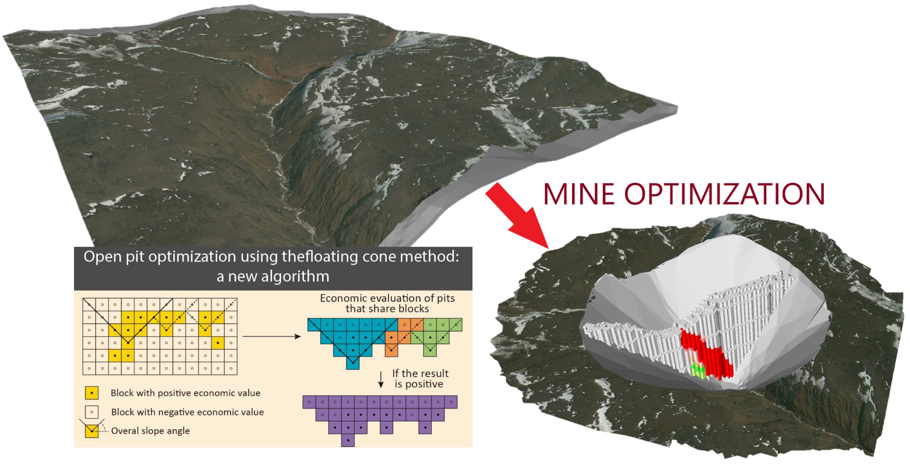
Open Pit Optimization Using the Floating Cone Method: A New Algorithm

 , , ,
, , ,
Abstract
:
1. Introduction
2. Block Models and Cut-Off Grade
3. Economic Pit Calculation Methods
4. Evolution of the Floating Cone Algorithm
4.1. Original Floating Cone
4.2. Floating Cone II
4.2.1. Modified Floating Cone II, Method 1
4.2.2. Modified Floating Cone II, Method 2
4.3. Floating Cone III
- The algorithm is very similar to the original floating cone algorithm, with the exception that when a cone is removed, the algorithm starts over from the first level. This step ends when all of the independent effective blocks in the model blocks have identified.
- Levels are analyzed for their effect on each other, e.g., an ore block on overlapping levels can make blocks of ore on underlying levels more or less effective.
- Following the technical restrictions, cones are built for all ore blocks and ore blocks are classified as dependent or independent.
- Ineffective independent blocks are identified. These blocks have negative cone value, though they can still form part of a positive block cone.
- Ineffective and dependent blocks, i.e., the blocks which have negative cone value, are identified. These blocks can be part of the final pit, but only as part of a larger cone, or together with other positive value blocks.
- Finally, the algorithm studies the remaining positive blocks. To do this, the algorithm continues as follows:
- Identify common blocks for each cone and calculate their weights. The weight of a block equals the number of cones in which said block can be included.
- Calculate the weight of cones. The weight of cone is the sum weight of common blocks of the cone.
- Calculate the value of the cone for each cone.
- Find the importance of each cone. The importance is the ratio between the weight of cones (which is the sum of the weight of the blocks that make up the cone) and cone value.
- Rank the cones at each level in order of importance, then by value in descending order.
- Extract the cones from each level in ascending order, adding the accumulated value.
- If the maximum accumulated value is positive, include the cones as part of the optimal pit. Repeat steps e–g for all levels of the model.
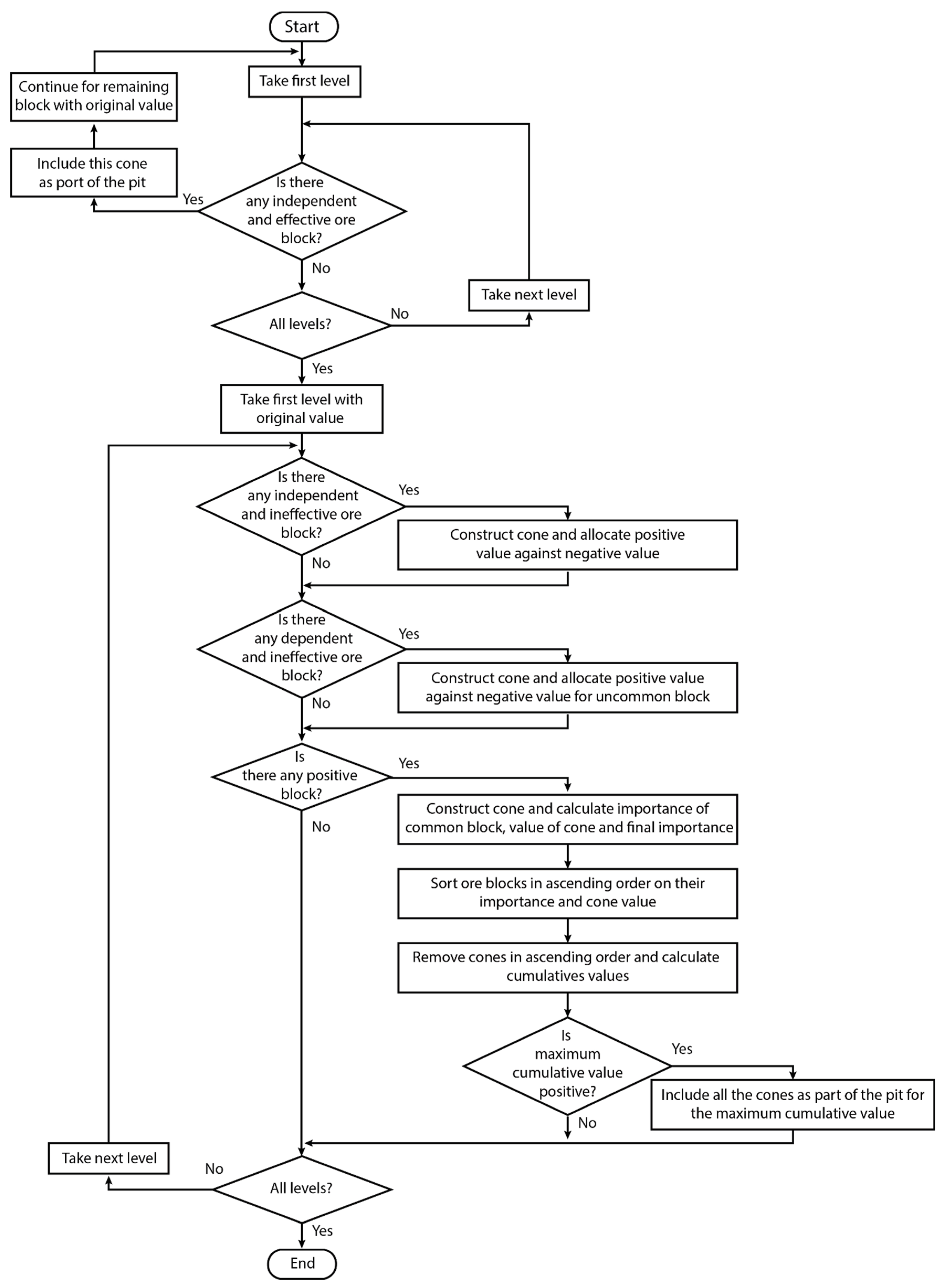
5. Floating Cone IV
- First, the algorithm reads the block model and assigns a value to each block according to Equation (3).
- In the first part, cones that are positive are removed from the block model following a strict order from top to bottom, taking into account that each time a cone is removed from the set, the process is restarted from the beginning, thus avoiding cones that are profitable due to the positive value of another cone that is above it. Once the first part is finished, the value of all the remaining cones in the block model will be negative.
- In the second part, the blocks with positive values are crossed again one by one from top to bottom. For each block with a positive value, it will calculate the value of the corresponding cone, which it will call the “cone under study”. If its value is positive, it is removed from the set and this second part is restarted again. The value of these cones should be negative, since the positives were removed in the first part, but when a cone is removed from the set in this second part, it is possible that some cone becomes positive if they have removed blocks that subtracted value, which is why it is returned to ask if the cone is positive before continuing with the process.
- If the value of the “cone under study” is negative, all positive value blocks that are at the same level or higher whose cones share blocks with the “cone under study” will be selected, ordered from top to bottom, and studied one by one if the value of the corresponding cone, removing the blocks that they share, is > = 0. When the first one that fulfills this condition is identified, it join its blocks, excluding those that they share so as not to repeat them, to the “cone under study”. If the value of the “cone under study” is already positive, it will be removed from the set and the second part will be restarted again. If it is still negative, it will continue with the rest of the selected blocks, repeating the process each time until one with a positive value is found, removing the common ones. If all of the selected blocks have been analyzed and the value of the “cone under study” is still negative, it will go on to the next block with a positive value.
- When all the blocks with a positive value have been studied in this second part without removing more cones from the set, the process will end. All the blocks that have been removed from the block model will be those that form the ultimate pit limit.
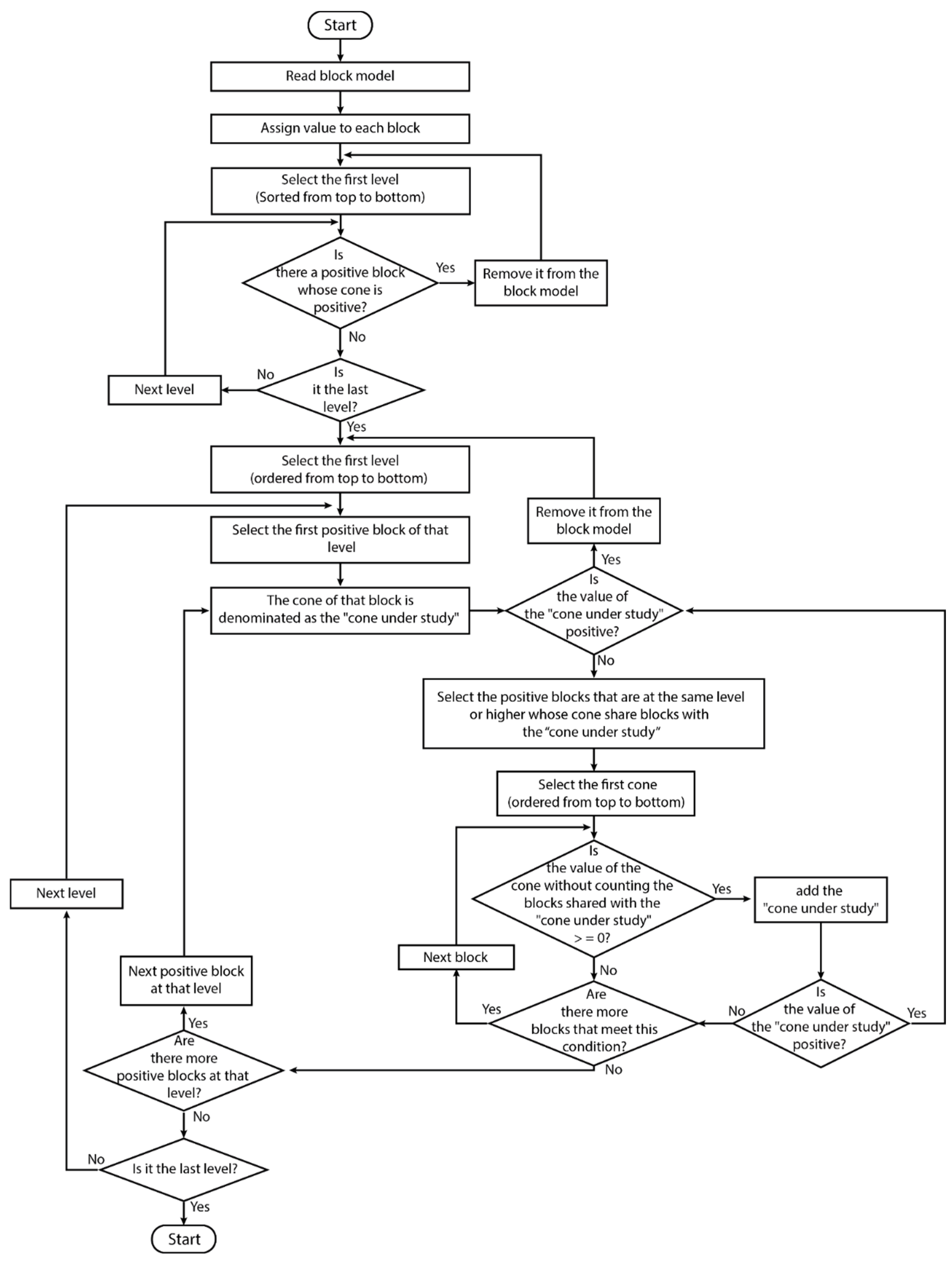
- First, the algorithm analyzes the block model and assigns a value to each block according to Equation (3).
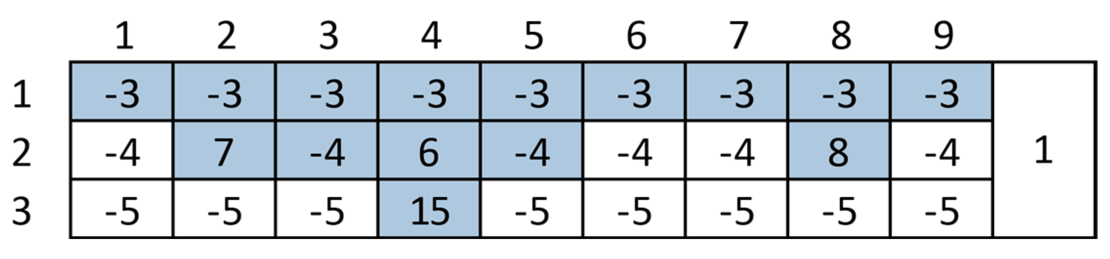
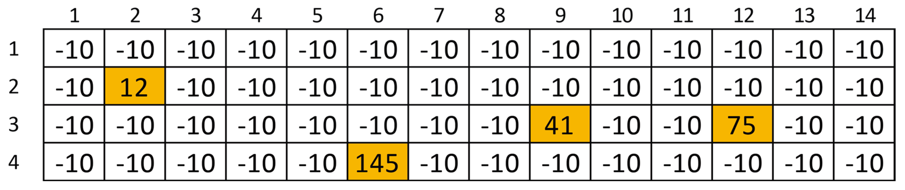
- Once the value of each block that makes up the model has been calculated, the algorithm follows the same logic as the original floating cone algorithm, as explained above. In this step, cones that are positive are removed from the block model following a strict order from top to bottom. Each time a cone is removed, the process is restarted from the beginning, thus avoiding cones that are profitable due to the positive value of another cone that is above it. In the block model of Figure 12, there is no single cone with a positive result.
- The remaining cones in the block model will all be negative, otherwise they would have been removed in the previous step. Each of these cones are known as the “cone under study”.
- The first “cone under study” will be selected and the cones prior to this one (which are above or at the same level) that share blocks with the “cone under study” will be studied. This study will always follow a descending order. In the block model shown in Figure 12, the first “cone under study” would be the cone of block (2, 2) but there are no previous cones or at the same level that share blocks.
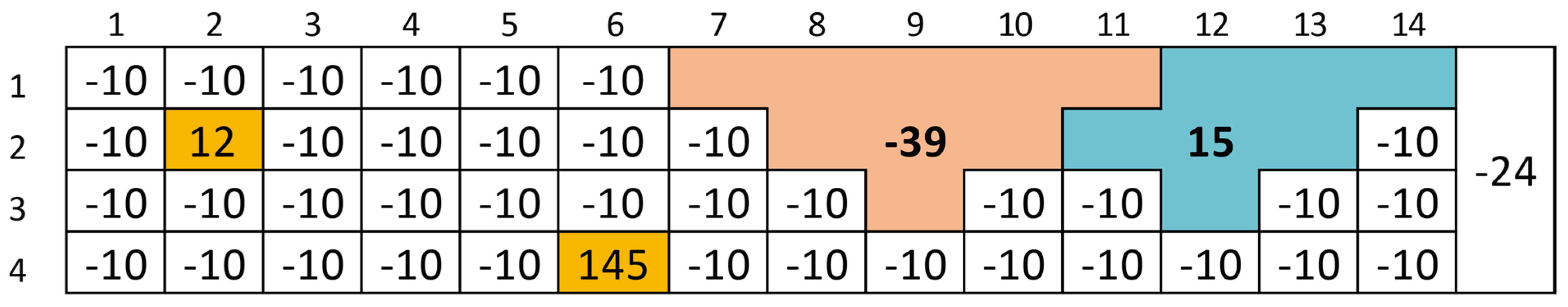
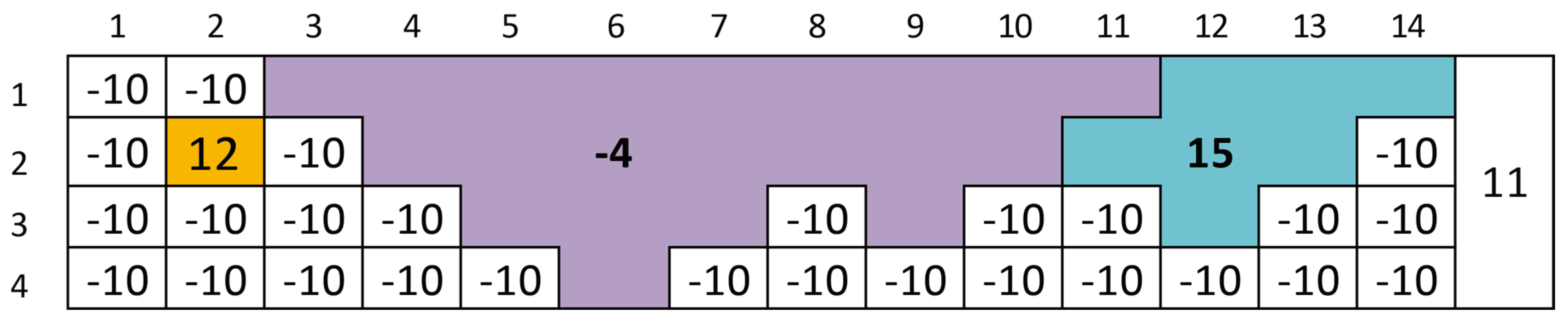
- The next “cone under study” would be the cone formed by the block (3, 9). In this case, it would share blocks with the cone formed by block (3, 12). The value of this second cone (Figure 13), without taking into account the blocks shared with the “cone under study”, would be positive (+15); however, the sum of both cones would still remain negative (-25). Since there are no other cones above or at the same level that share blocks with the cone under study, the next “cone under study” would be passed.
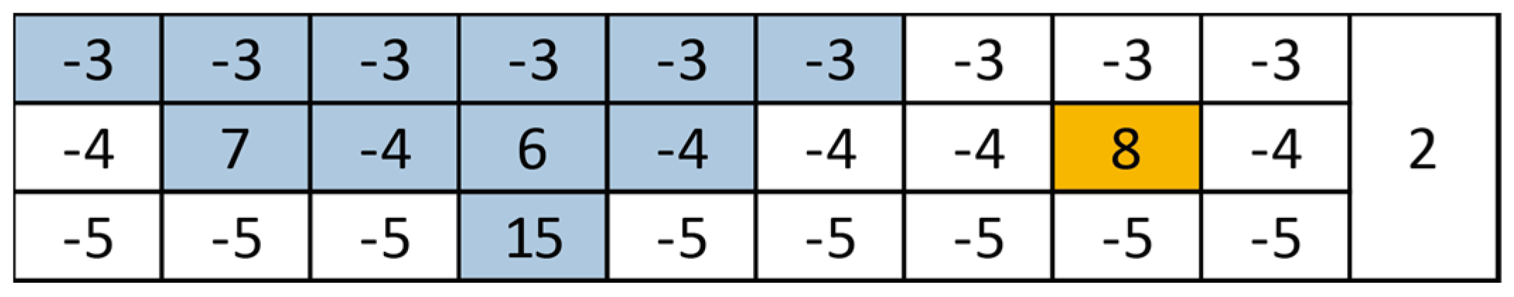
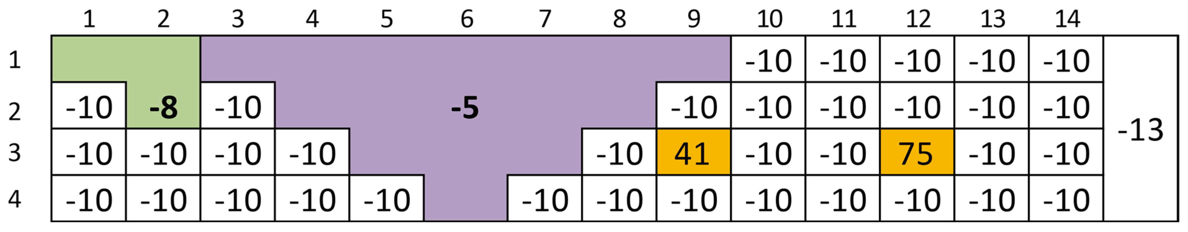
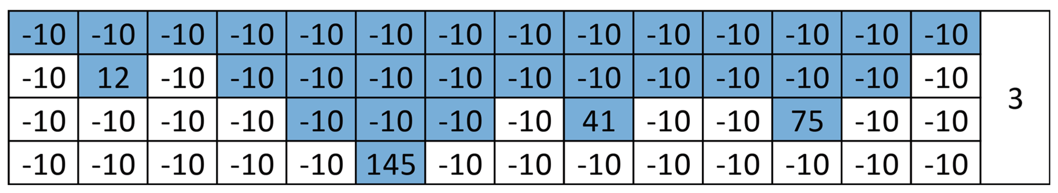
- The last “cone under study” that remains to be analyzed would be that of the block (4, 6). The first cone that it will share blocks with would be the block cone (2, 2). As can be seen in Figure 14, the value of this second cone, without taking into account the blocks shared with the “cone under study”, is negative (−8), so it is not incorporated into the “cone under study”.
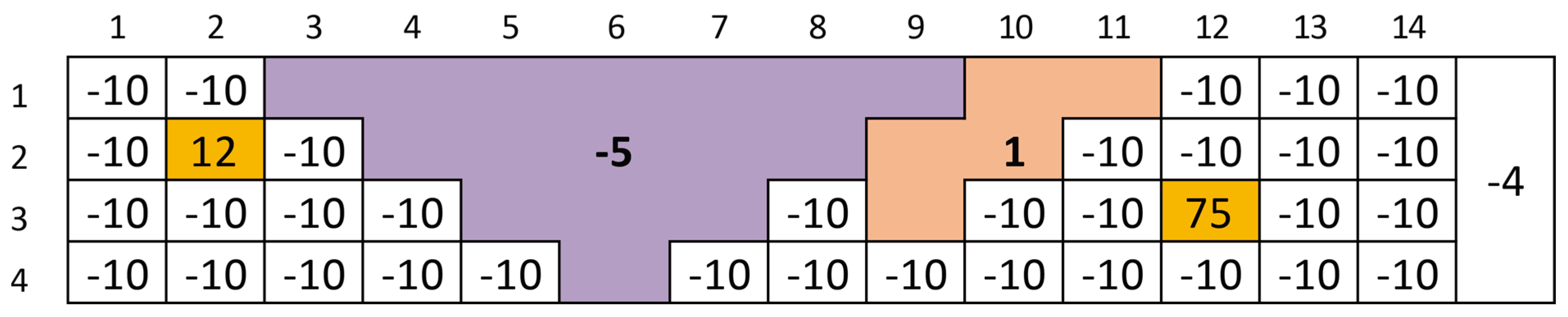
- The next cone with which the “cone under study” would share blocks would be the cone of the block (3, 9), as shown in Figure 15. In this case, the value of this second cone, not counting the shared blocks with the “cone under study”, is positive (+1), so it is added to the “cone under study” (Figure 15).
- The new “cone under study” shares blocks with the cone of the block (3, 12). The value of this second cone, not counting the blocks shared with the “cone under study”, is positive (+15) so it would be added to the cone under study (Figure 16). As the “cone under study” is now positive (+11), it is removed from the block model. In the event that the sum of the cones are negative and there are no more cones with which the “cone under study” shares blocks, it would be discarded and the next “cone under study” would be passed. If there is no other “cone under study”, as in this block model, the process will end.
6. Comparison of the Different Algorithms of the Floating Cone
- Weight of each block (the number of cones in which said block can be included);
- Weight of the cones (the sum of the weights of all the blocks within each cone);
- Value of the different cones;
- Importance of each cone (the relationship between the weight of the cones and the value of the cone).
7. Floating Cone IV versus Lerchs–Grossmann
- Conceptual study: ±30%
- Preliminary study: ±20%
- Feasibility study: ±10%
8. Conclusions
- The calculation of the ultimate pit limit must consider a study of robustness or sensitivity to changes in market conditions, mainly the sale price.
- The optimal pit defined by the different methods is the basis for designing the final pit in which the transport lanes are included. Therefore, the actual log will implement more blocks in the contour. The floating cone method when making slightly larger pits would already include blocks for the design of the ramps.
- The geological uncertainty in these stages is greater than the differences between the different methods of calculating the optimal pit.
- During the mining operation, changes will occur (problems during execution, changes in the market, application of reserves, etc.) that will modify the design of the mine with respect to the ultimate pit limit calculated in these stages.
Author Contributions
Funding
Institutional Review Board Statement
Informed Consent Statement
Data Availability Statement
Conflicts of Interest
References
- Hartman, H.L. SME Mining Engineering Handbook; Society for Mining, Metallurgy, and Exploration: Denver, CO, USA, 1992. [Google Scholar]
- Khalokakaie, R.; Dowd, P.A.; Fowell, R.J. Lerchs–Grossmann algorithm with variable slope angles. Min. Technol. 2000, 109, 77–85. [Google Scholar] [CrossRef]
- Khalokakaie, R.; Dowd, P.A.; Fowell, R.J. A Windows program for optimal open pit design with variable slope angles. Int. J. Surf. Min. Reclam. Environ. 2000, 14, 261–275. [Google Scholar] [CrossRef]
- Pana, M.T. The simulation approach to open pit design. In Proceedings of the 5th Symposium on the Application of Computers and Operations Research in the Mineral Industries (APCOM), Tucson, Arizona, USA, 10–11 March 1965; pp. ZZ1–ZZ24. [Google Scholar]
- Carlson, T.R.; Erickson, J.D.; O’Brain, D.T.; Pana, M.T. Computer techniques in mine planning. Min. Eng. 1966, 18, 53–56. [Google Scholar]
- David, M.; Dowd, P.A.; Korobov, S. Forecasting departure from planning in open pit design and grade control. In Proceedings of the 12th Symposium on the Application of Computers and Operations Research in the Mineral Industries (APCOM), Boulder, CO, USA, April 1974; pp. F131–F142. [Google Scholar]
- Dowd, P.A.; Onur, A.H. Open-pit optimization. 1. Optimal open-pit design. Trans. Inst. Min. Metall. 1993, 102, A95–A104. [Google Scholar]
- Lerchs, H. Optimum design of open-pit mines. Trans CIM 1965, 68, 17–24. [Google Scholar]
- Wright, A. MOVING CONE II-A simple algorithm for optimum pit limits design. In Proceedings of the 28th Symposium on the Application of Computers and Operations Research in the Mineral Industries (APCOM), Golden, CO, USA, 20–22 October 1999; pp. 367–374. [Google Scholar]
- Khalou, K.R. Optimum Open Pit Design with Modified Moving Cone II Methods. J. Fac. Eng. 2007, 41, 297–307. [Google Scholar]
- Elahi, E.; Kakaie, R.; Yusefi, A. A new algorithm for optimum open pit design: Floating cone method III. J. Min. Environ. 2012, 2, 118–125. [Google Scholar] [CrossRef]
- Díaz, A.B.; Álvarez, I.D.; Fernández, C.C.; Krzemień, A.; Rodríguez, F.J.I. Calculating ultimate pit limits and determining pushbacks in open-pit mining projects. Resour. Policy 2021, 72, 102058. [Google Scholar] [CrossRef]
- Githiria, J.; Musingwini, C. Comparison of cut-off grade models in mine planning for improved value creation based on NPV. In Proceedings of the 6th Regional Conference of the Society of Mining Professors (SOMP), Johannesburg, South Africa, 12–13 March 2018; pp. 347–362. [Google Scholar]
- Khan, A.; Asad, M.W.A. A method for optimal cut-off grade policy in open pit mining operations under uncertain supply. Resour. Policy 2019, 60, 178–184. [Google Scholar] [CrossRef]
- Lane, K.F. The Economic Definition of Ore: Cut-off Grades in Theory and Practice; Mining Journal Books Limited: London, UK, 1988. [Google Scholar]
- Bai, X.; Turczynski, G.; Baxter, N.; Place, D.; Sinclair-Ross, H. Pseudoflow method for pit optimization. In Whitepaper Geovia Whittle Dassault Systems; Dassault Systemes: Waltham, MA, USA, 2017. [Google Scholar]
- Koenigsberg, E. The optimum contours of an open pit mine: An application of dynamic programming. In Proceedings of the 17th Application of Computers and Operations Research in the Mineral Industry (APCOM), New York, NY, USA, 19–22 April 1982; pp. 274–287. [Google Scholar]
- Wilke, F.L. Determining the Optimal Untimate Pit Design for Hard Rock Open Pit Mines Using Dynamic Programming. Erzmetal 1984, 37, 139–144. [Google Scholar]
- Yamatomi, J.; Mogi, G.; Akaike, A.; Yamaguchi, U. Selective extraction dynamic cone algorithm for three-dimensional open pit designs. In Proceedings of the 25th Symposium on the Application of Computers and Operations Research in the Mineral Industries (APCOM), Brisbane, Australia, 9–14 July 1995; Australasian Institute of Mining and Metallurgy: Carlton, VIC, Australia, 1995; pp. 267–274. [Google Scholar]
- Denby, B.; Schofield, D. Open-pit design and scheduling by use of genetic algorithms. Trans. Inst. Min. Metall. 1994, 103, A21–A26. [Google Scholar]
- García, M.V.R.; Krzemień, A.; Bárcena, L.C.S.; Álvarez, I.D.; Fernández, C.C. Scoping studies of rare earth mining investments: Deciding on further project developments. Resour. Policy 2019, 64, 101525. [Google Scholar] [CrossRef]
- Cambon, J. Hudson Receives New Sarfartoq Rare Earth and Niobium Exploration License. Hudson Resources Inc. 9 March 2020. Available online: https://hudsonresourcesinc.com/hudson-receives-new-sarfartoq-rare-earth-and-niobium-exploration-license/ (accessed on 30 January 2022).
- Akisa, D.M.; Mireku-Gyimah, D. Application of surpac and whittle software in open pit optimisation and design. Ghana Min. J. 2015, 15, 35–43. [Google Scholar]
- Lee, T.D. Planning and mine feasibility study–An owner perspective. In Proceedings of the 1984 NWMA Short Course “Mine Feasibility–Concept to Completion”, Spokane, WA, USA, 15–17 April 1984. [Google Scholar]
- Dominy, S.C.; Noppé, M.A.; Annels, A.E. Errors and uncertainty in mineral resource and ore reserve estimation: The importance of getting it right. Explor. Min. Geol. 2002, 11, 77–98. [Google Scholar] [CrossRef]
- David, M. Geostatistical Ore Reserve Estimation; Elsevier: Amsterdam, The Netherlands, 1977. [Google Scholar]
- David, M. Handbook of Applied Advanced Geostatistical Ore Reserve Estimation; Elsevier: Amsterdam, The Netherlands, 1988. [Google Scholar]
- Annels, A.E. Mineral Deposit Evaluation: A Practical Approach; Springer: Berlin/Heidelberg, Germany, 2012. [Google Scholar]


| Stage | Block | Block Value | Cone Value | Cumulative Value | Mineable? |
|---|---|---|---|---|---|
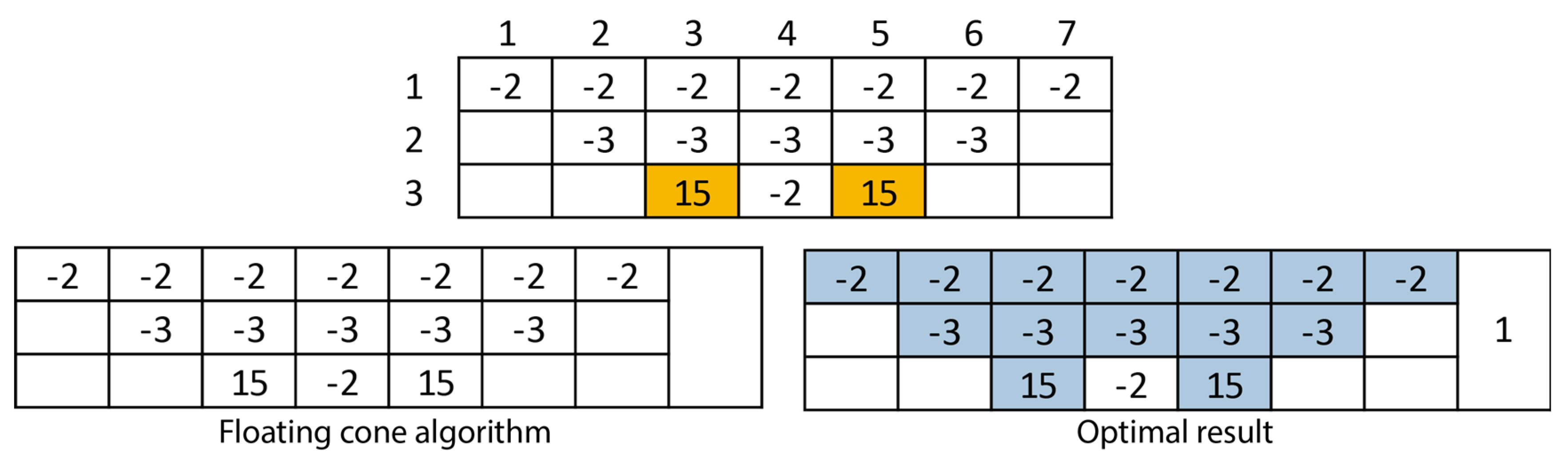
| 3 | (3, 3) | +15 | −4 | −4 | No |
| (3, 5) | +15 | +5 | +1 | Yes |
| Stage | Block | Block Value | Cone Value | Cumulative Value | Mineable? |
|---|---|---|---|---|---|
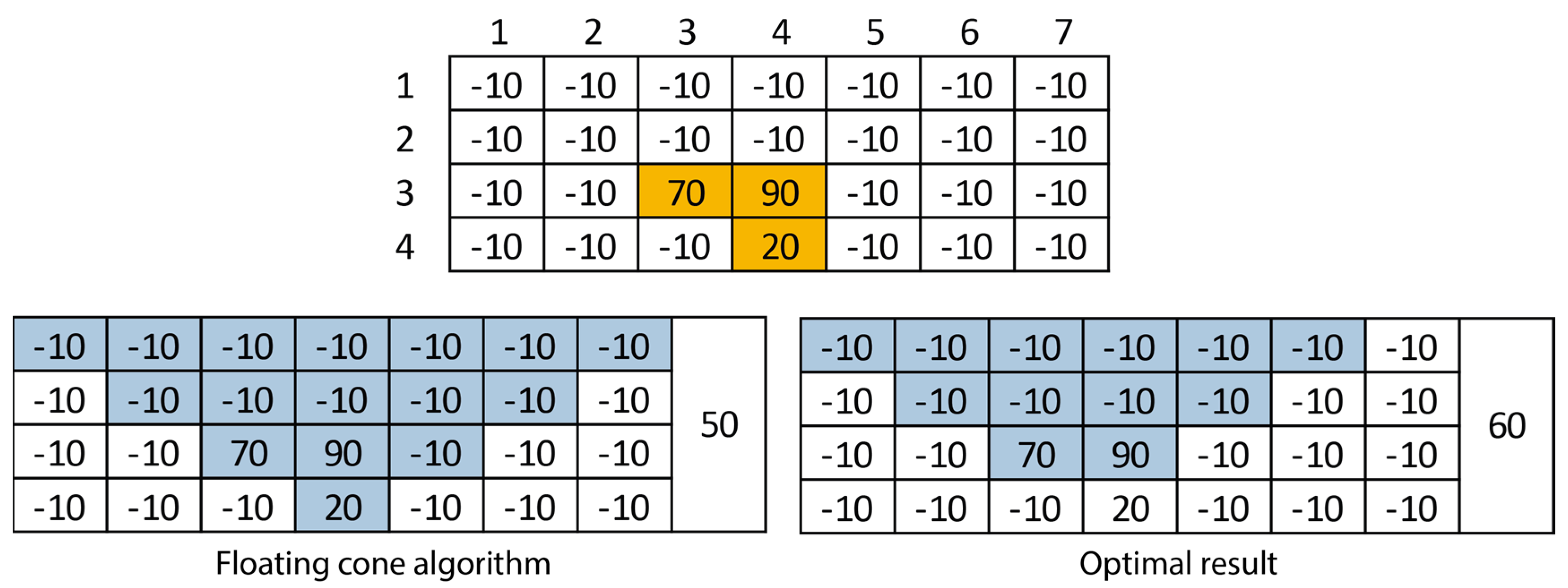
| 3 | (3, 3) | +70 | −10 | −10 | No |
| (3, 4) | +90 | +70 | +60 | Yes | |
| 4 | (4, 4) | +20 | −10 | +50 | Yes, but not optimal |
| Stage | Block | Block Value | Cone Value | Cumulative Value | Mineable? |
|---|---|---|---|---|---|
| 2 | (2, 8) | +8 | −1 | −1 | No |
| (2, 2) | +7 | −2 | −3 | No | |
| (2, 4) | +6 | 0 | −3 | No | |
| 3 | (3, 4) | +15 | −2 | −2 | No |
| Stage | Block | Block Value | Cone Value | Cumulative Value | Mineable? |
|---|---|---|---|---|---|
| 2 | (2, 8) | +8 | −1 | −1 | No |
| (2, 2) | +7 | −2 | −3 | No | |
| 3 | (3, 4) | +15 | +4 | +1 | Yes |
| Stage | Block | Block Value | Cone Value | Cumulative Value | Mineable? |
|---|---|---|---|---|---|
| 2 | (2, 2) | +12 | −18 | −18 | No |
| 3 | (3, 12) | +75 | −5 | −5 | No |
| (3, 9) | +41 | −39 | −24 | No | |
| 4 | (4, 6) | +145 | −5 | −5 | No |
| Stage | Block | Block Value | Cone Value | Cumulative Value | Mineable? |
|---|---|---|---|---|---|
| 2 | (2, 2) | +12 | −18 | −18 | No |
| 3 | (3, 12) | +75 | −5 | −23 | No |
| (3, 9) | +41 | −39 | −24 | No | |
| 4 | (4, 6) | +145 | −5 | +3 | Yes |
| Date | Lerchs–Grossmann | Floating Cone | Floating Cone IV |
|---|---|---|---|
| No. of pit blocks | 53,021 | 58,211 | 55,901 |
| No. of ore blocks | 5322 | 5324 | 5313 |
| No. of waste blocks | 47,699 | 52,887 | 50,588 |
| Calculation time | 3 min 2 s | 9 min 47 s | 3 min 59 s |
| Pit volume (m3) | 53,021,000.00 | 58,211,000.000 | 55,901,000.000 |
| Pit weight (t) | 159,063,000.00 | 174,633,000.000 | 167,703,000.00 |
| Ore weight (t) | 15,966,000.00 | 15,972,000.000 | 15,939,000.00 |
| Waste weight (t) | 143,097,000.00 | 158,661,000.000 | 151,764,000.000 |
| Ratio | 8.963 | 9.934 | 9.522 |
| cut-off grade (%) | 1.201 | 1.201 | 1.201 |
| Metal (t) | 191,751.66 | 191,823.72 | 191,427.39 |
| Recovered Metal (t) | 146,939.30 | 146,994.52 | 146,690.81 |
| Meta value ($) | 4,918,058,272.531 | 4,919,906,471.807 | 4,909,741,375.79 |
| Ore mining cost ($) | 40,872,960.000 | 40,888,320.000 | 40,803,840.00 |
| Waste mining cost ($) | 366,328,320.000 | 406,172,160.000 | 388,515,840.00 |
| Processing cost ($) | 1,918,793,880.000 | 1,919,514,960.000 | 1,915,549,020.00 |
| Total cost ($) | 2,325,995,160.00 | 2,366,575,440.00 | 2,344,868,700.00 |
| Income less cost ($) | 2,592,063,112.531 | 2,553,331,031.807 | 2,564,872,675.79 |
Publisher’s Note: MDPI stays neutral with regard to jurisdictional claims in published maps and institutional affiliations. |
© 2022 by the authors. Licensee MDPI, Basel, Switzerland. This article is an open access article distributed under the terms and conditions of the Creative Commons Attribution (CC BY) license (https://creativecommons.org/licenses/by/4.0/).
Share and Cite
Ares, G.; Castañón Fernández, C.; Álvarez, I.D.; Arias, D.; Díaz, A.B. Open Pit Optimization Using the Floating Cone Method: A New Algorithm. Minerals 2022, 12, 495. https://doi.org/10.3390/min12040495
Ares G, Castañón Fernández C, Álvarez ID, Arias D, Díaz AB. Open Pit Optimization Using the Floating Cone Method: A New Algorithm. Minerals. 2022; 12(4):495. https://doi.org/10.3390/min12040495
Chicago/Turabian StyleAres, Gonzalo, César Castañón Fernández, Isidro Diego Álvarez, Daniel Arias, and Arturo Buelga Díaz. 2022. "Open Pit Optimization Using the Floating Cone Method: A New Algorithm" Minerals 12, no. 4: 495. https://doi.org/10.3390/min12040495