
Deep-Learning-Based Automatic Mineral Grain Segmentation and Recognition


Abstract
:1. Introduction
2. Literature Review
2.1. Traditional, Device-Based Methods
2.2. Computer Vision-Based Computational Methods
3. Materials and Methods
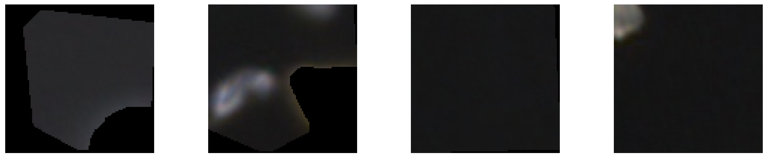
3.1. Data Set Acquisition
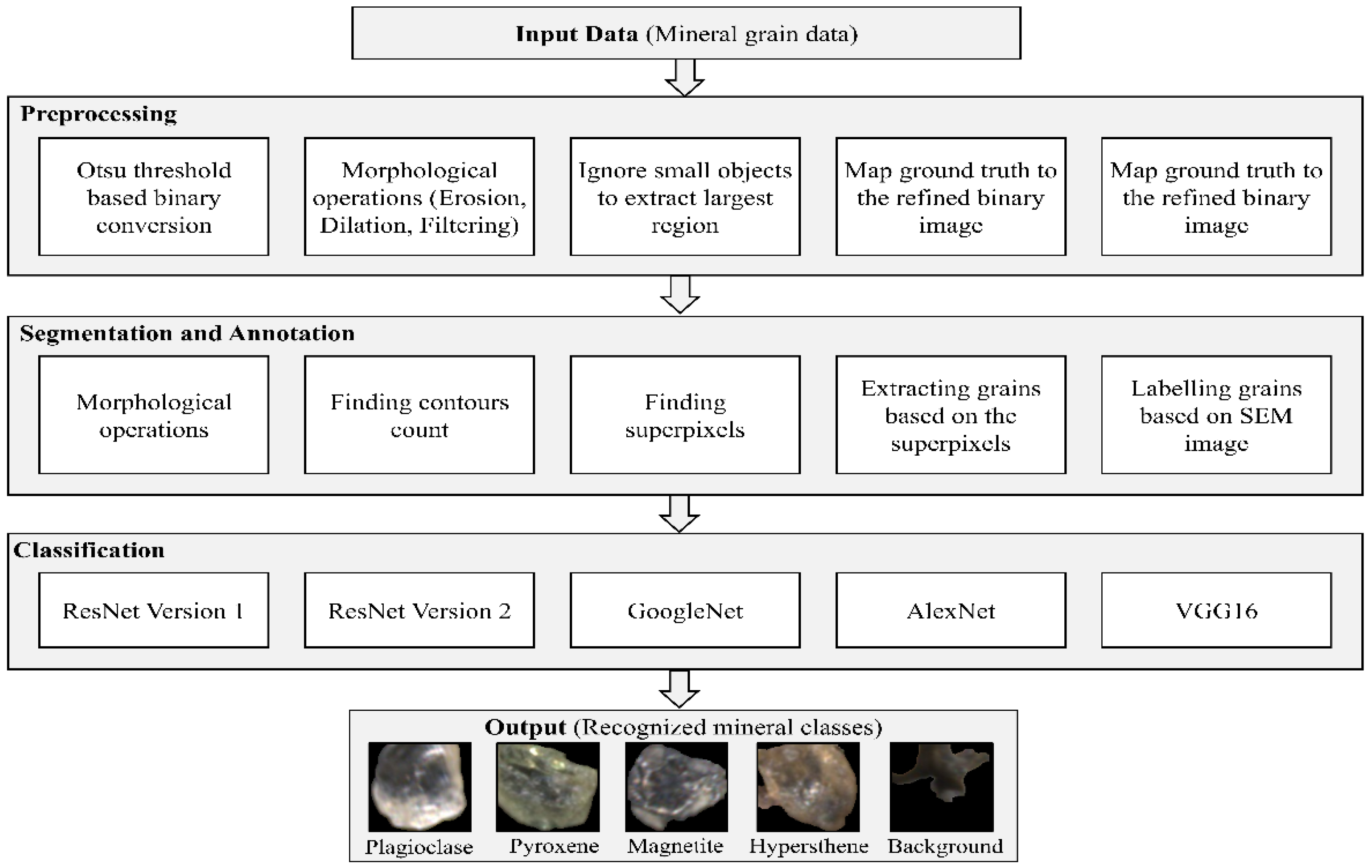
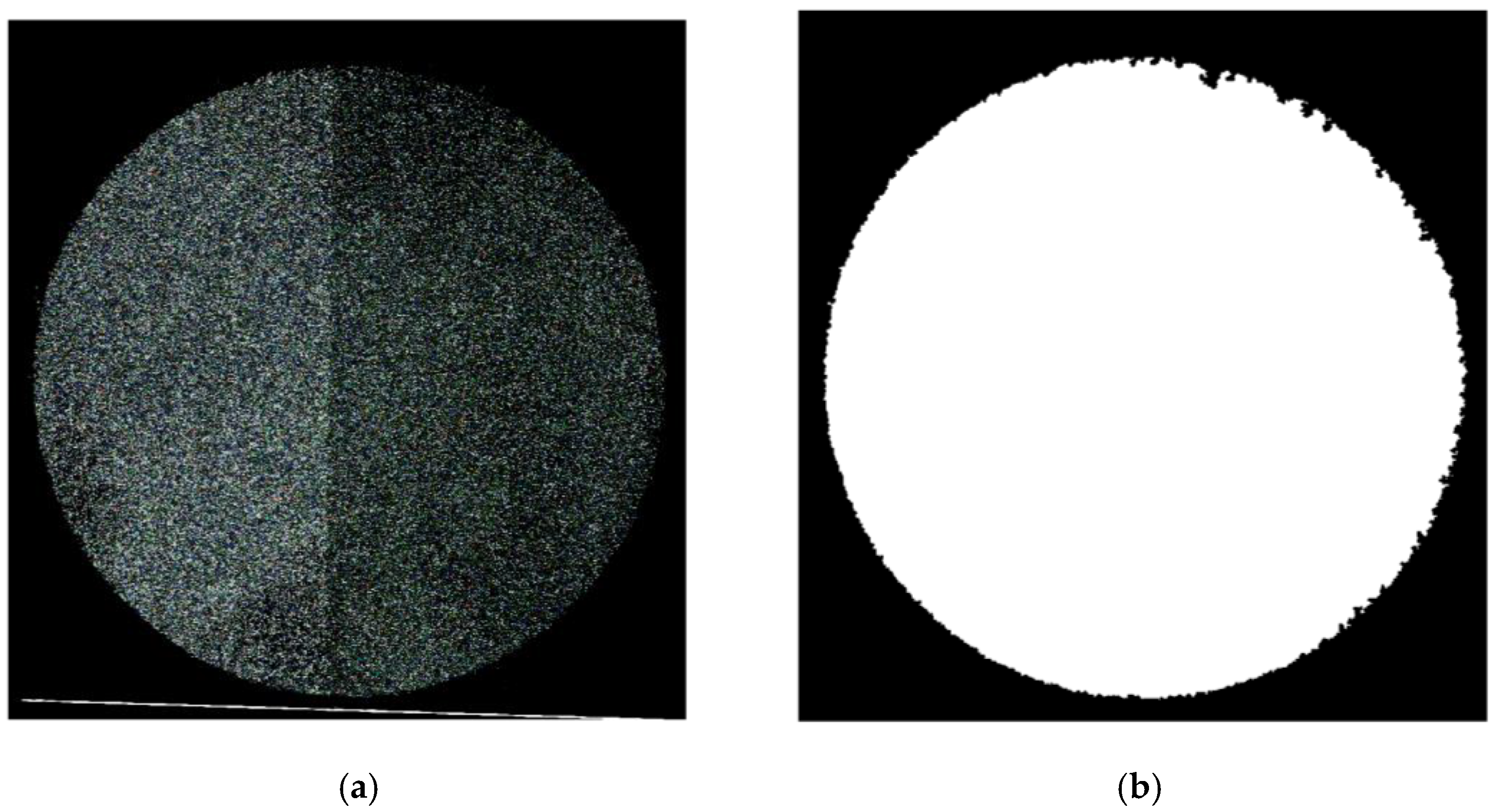
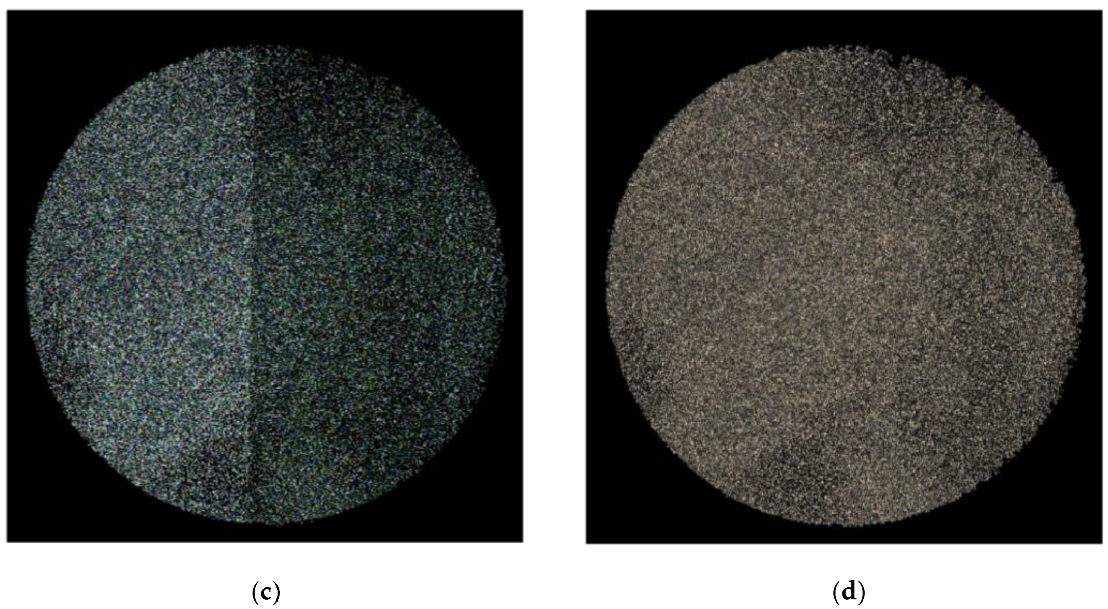
3.2. Data Preprocessing
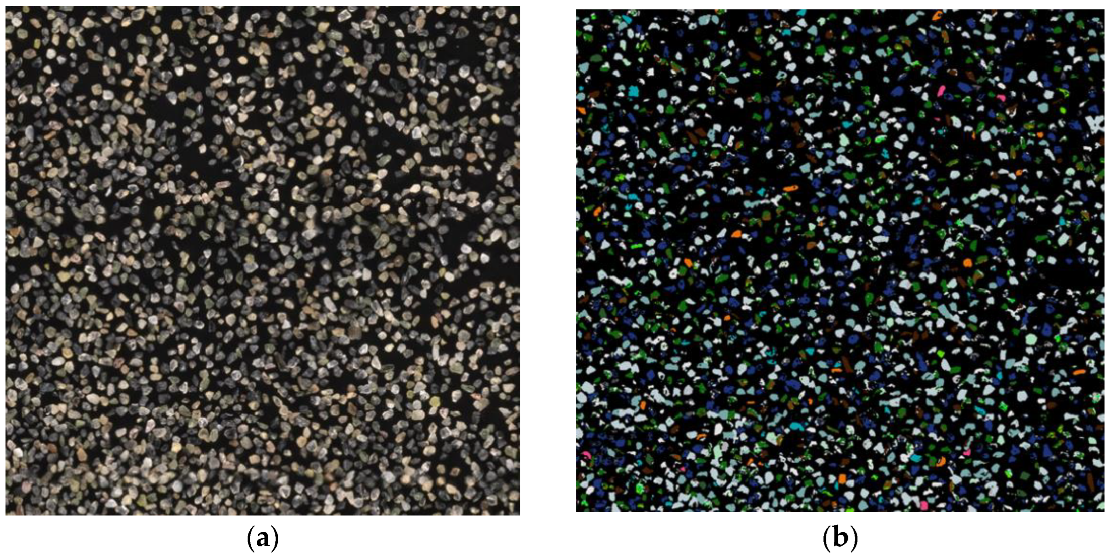
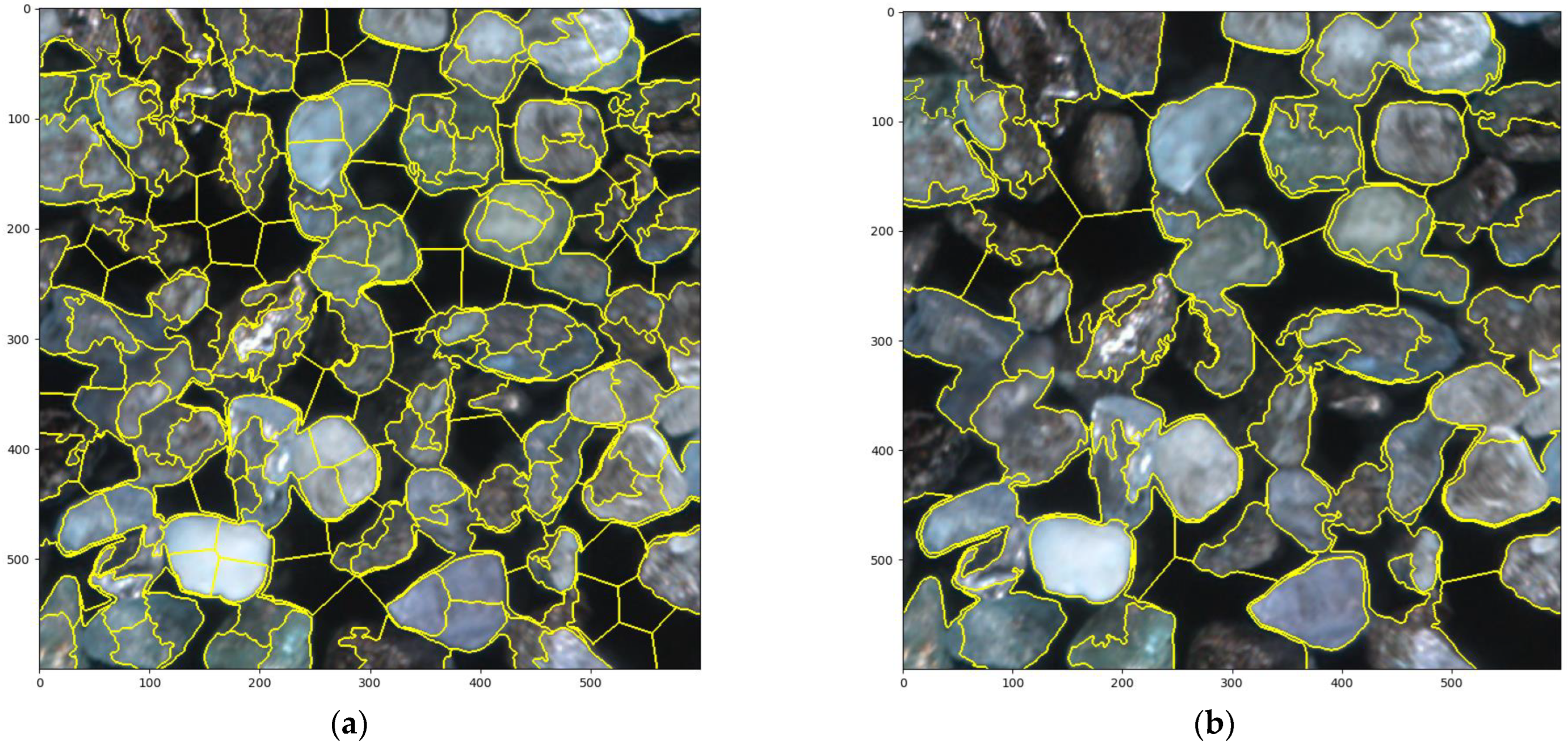
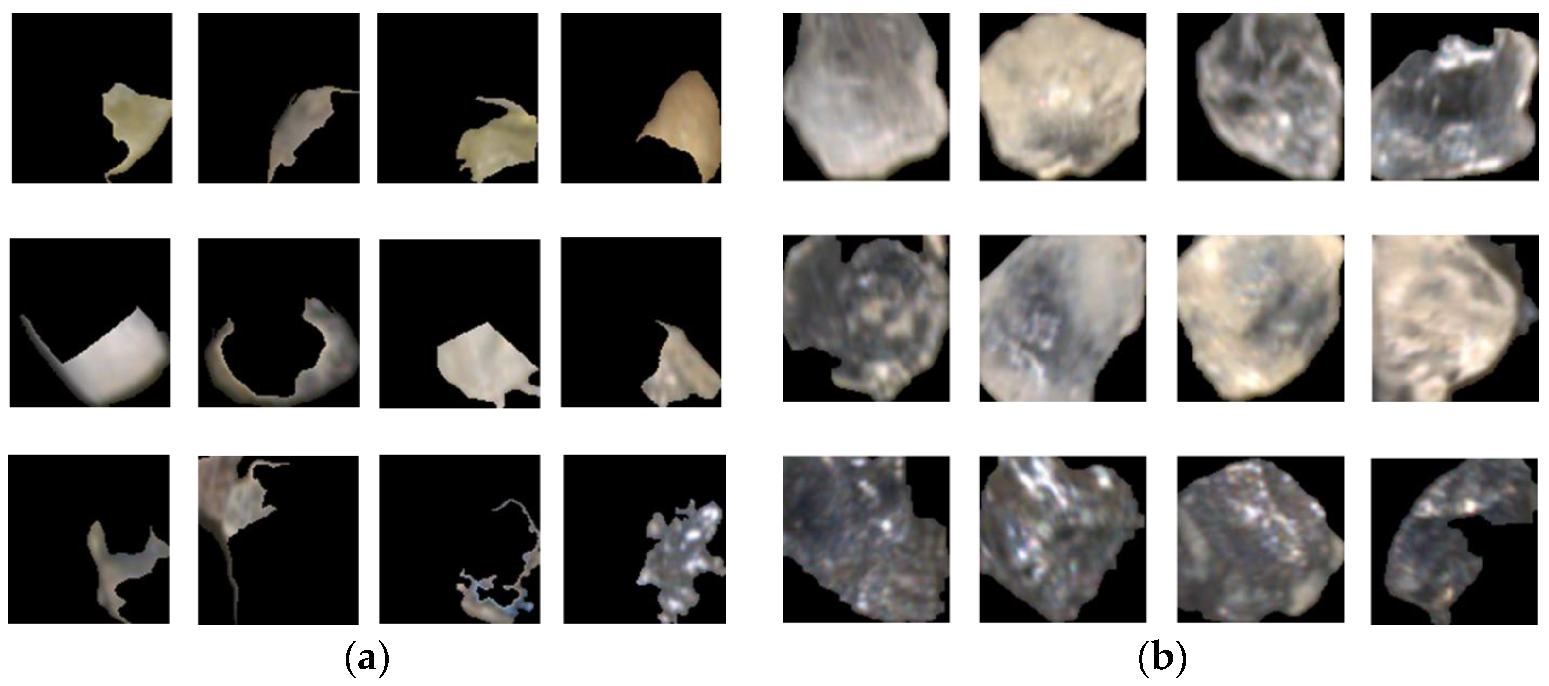
3.3. Grain Segmentation
| Algorithm 1: Segmentation and Annotation of Grains |
| Input: Grains mosaic image with BSE groundtruthing image and classes Output: Segmented grains with their annotation read , read ← binary (grayscale (), Otsu) ← erosion ( ← find external contours (, chain approx simple) ← length () GrainsApprox ← ← histogram equalization () ← superpixel () ← unique colors ← 0 for in ← if for in ← ← , else ← 0 ← end for |
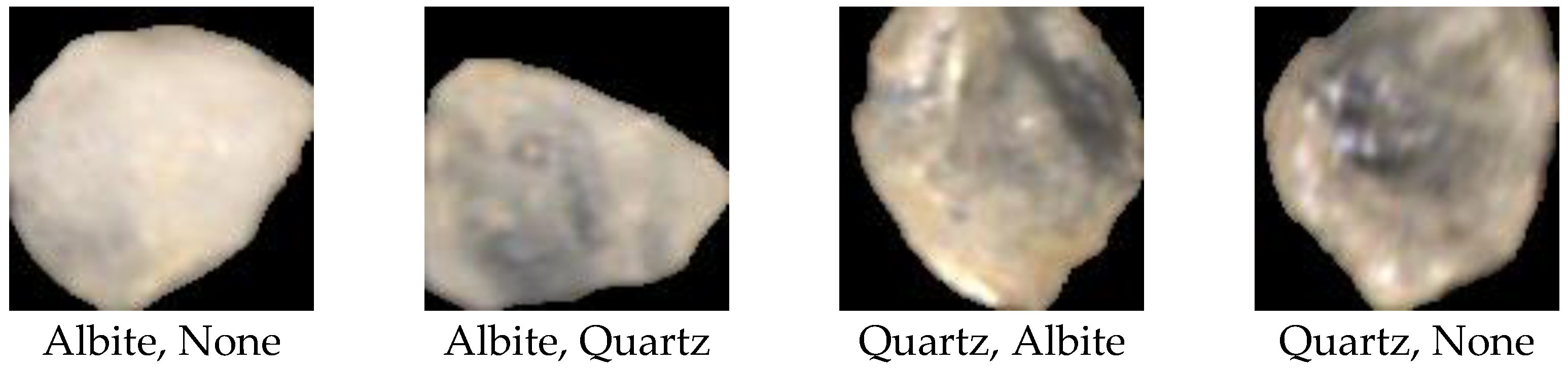
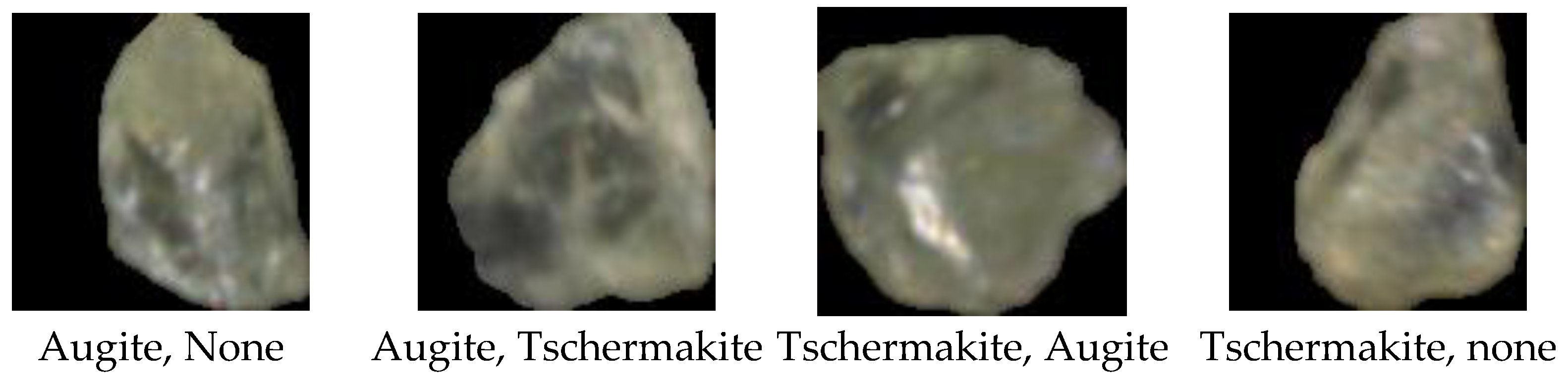
3.4. Grain Class Annotation
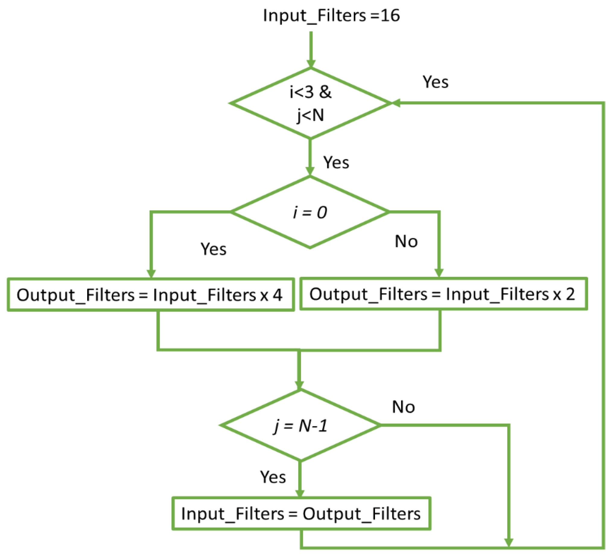
3.5. ResNet Models for Grain Recognition
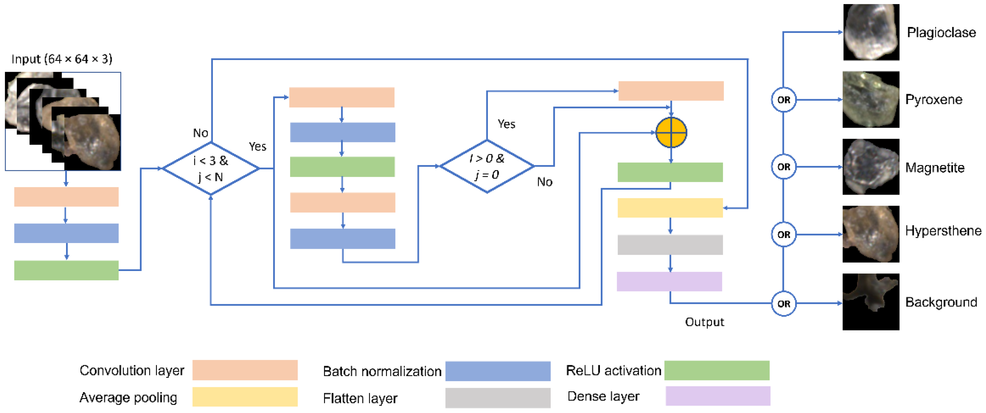
3.5.1. ResNet Version 1
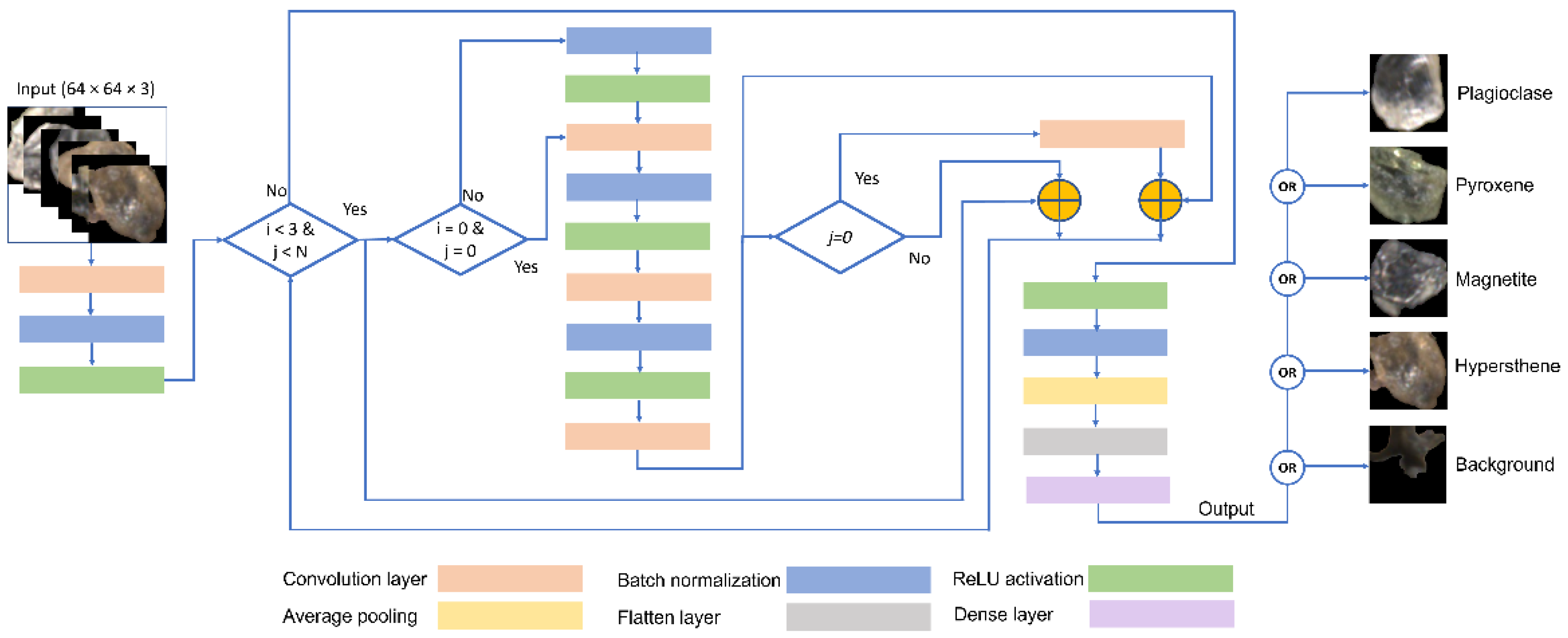
3.5.2. ResNet Version 2
4. Experimental Results
5. Discussion and Conclusions
- The scarcity of mineral data sets. A key contribution of this work is the development of such a data set, because they are not readily available for grain mineral classification.
- Unbalanced data for different classes. In the developed data set, there was an unequal number of images available for each class.
- High-performance GPUs are required for training. We had access to a GPU system; however, the training step required a considerable amount of time to be performed.
Author Contributions
Funding
Data Availability Statement
Acknowledgments
Conflicts of Interest
References
- Jung, D.; Choi, Y. Systematic Review of Machine Learning Applications in Mining: Exploration, Exploitation, and Reclamation. Minerals 2021, 11, 148. [Google Scholar] [CrossRef]
- Sengupta, S.; Dave, V. Predicting applicable law sections from judicial case reports using legislative text analysis with machine learning. J. Comput. Soc. Sci. 2021, 1–14. [Google Scholar] [CrossRef]
- Zantalis, F.; Koulouras, G.; Karabetsos, S.; Kandris, D. A Review of Machine Learning and IoT in Smart Transportation. Future Internet 2019, 11, 94. [Google Scholar] [CrossRef] [Green Version]
- Latif, G.; Shankar, A.; Alghazo, J.; Kalyanasundaram, V.; Boopathi, C.S.; Jaffar, M.A. I-CARES: Advancing health diagnosis and medication through IoT. Wirel. Netw. 2019, 26, 2375–2389. [Google Scholar] [CrossRef]
- Ali, D.; Frimpong, S. Artificial intelligence, machine learning and process automation: Existing knowledge frontier and way forward for mining sector. Artif. Intell. Rev. 2020, 53, 6025–6042. [Google Scholar] [CrossRef]
- Chow, B.H.Y.; Reyes-Aldasoro, C.C. Automatic Gemstone Classification Using Computer Vision. Minerals 2021, 12, 60. [Google Scholar] [CrossRef]
- Girard, R.; Tremblay, J.; Néron, A.; Longuépée, H. Automated Gold Grain Counting. Part 1: Why Counts Matter! Minerals 2021, 11, 337. [Google Scholar] [CrossRef]
- Boivin, J.-F.; Bédard, L.P.; Longuépée, H. Counting a pot of gold: A till golden standard (AuGC-1). J. Geochem. Explor. 2021, 229, 106821. [Google Scholar] [CrossRef]
- Plouffe, A.; McClenaghan, M.B.; Paulen, R.C.; McMartin, I.; Campbell, J.E.; Spirito, W.A. Processing of glacial sediments for the recovery of indicator minerals: Protocols used at the Geological Survey of Canada. Geochem. Explor. Environ. Anal. 2013, 13, 303–316. [Google Scholar] [CrossRef]
- Xu, C.S.; Hayworth, K.J.; Lu, Z.; Grob, P.; Hassan, A.M.; García-Cerdán, J.G.; Niyogi, K.K.; Nogales, E.; Weinberg, R.J.; Hess, H.F. Enhanced FIB-SEM systems for large-volume 3D imaging. eLife 2017, 6, e25916. [Google Scholar] [CrossRef]
- Nie, J.; Peng, W. Automated SEM–EDS heavy mineral analysis reveals no provenance shift between glacial loess and interglacial paleosol on the Chinese Loess Plateau. Aeolian Res. 2014, 13, 71–75. [Google Scholar] [CrossRef]
- Akcil, A.; Koldas, S. Acid Mine Drainage (AMD): Causes, treatment and case studies. J. Clean. Prod. 2006, 14, 1139–1145. [Google Scholar] [CrossRef]
- Hudson-Edwards, K.A. Sources, mineralogy, chemistry and fate ofheavy metal-bearing particles in mining-affected river systems. Miner. Mag. 2003, 67, 205–217. [Google Scholar] [CrossRef]
- Hobbs, D.W. 4 Structural Effects and Implications and Repair. In Alkali-Silica Reaction in Concrete; Thomas Telford Publishing: London, UK, 1988; pp. 73–87. [Google Scholar] [CrossRef]
- Lawrence, P.; Cyr, M.; Ringot, E. Mineral admixtures in mortars effect of type, amount and fineness of fine constituents on compressive strength. Cem. Concr. Res. 2005, 35, 1092–1105. [Google Scholar] [CrossRef]
- Erlich, E.I.; Hausel, W.D. Diamond Deposits: Origin, Exploration, and History of Discovery; SME: Littleton, CO, USA, 2003. [Google Scholar]
- Towie, N.J.; Seet, L.H. Diamond laboratory techniques. J. Geochem. Explor. 1995, 53, 205–212. [Google Scholar] [CrossRef]
- Chen, Z.; Liu, X.; Yang, J.; Little, E.C.; Zhou, Y. Deep learning-based method for SEM image segmentation in mineral characterization, an example from Duvernay Shale samples in Western Canada Sedimentary Basin. Comput. Geosci. 2020, 138, 104450. [Google Scholar] [CrossRef]
- Hyder, Z.; Siau, K.; Nah, F. Artificial Intelligence, Machine Learning, and Autonomous Technologies in Mining Industry. J. Database Manag. 2019, 30, 67–79. [Google Scholar] [CrossRef]
- Dalm, M.; Buxton, M.W.; van Ruitenbeek, F.; Voncken, J.H. Application of near-infrared spectroscopy to sensor based sorting of a porphyry copper ore. Miner. Eng. 2014, 58, 7–16. [Google Scholar] [CrossRef]
- McCoy, J.; Auret, L. Machine learning applications in minerals processing: A review. Miner. Eng. 2018, 132, 95–109. [Google Scholar] [CrossRef]
- Maitre, J.; Bouchard, K.; Bedard, L. Mineral grains recognition using computer vision and machine learning. Comput. Geosci. 2019, 130, 84–93. [Google Scholar] [CrossRef]
- Makvandi, S.; Pagé, P.; Tremblay, J.; Girard, R. Exploration for Platinum-Group Minerals in Till: A New Approach to the Recovery, Counting, Mineral Identification and Chemical Characterization. Minerals 2021, 11, 264. [Google Scholar] [CrossRef]
- Kim, C.S. Characterization and speciation of mercury-bearing mine wastes using X-ray absorption spectroscopy. Sci. Total Environ. 2000, 261, 157–168. [Google Scholar] [CrossRef] [Green Version]
- Baklanova, O.; Shvets, O. Cluster analysis methods for recognition of mineral rocks in the mining industry. In Proceedings of the 2014 4th International Conference on Image Processing Theory, Tools and Applications (IPTA), Paris, France, 14–17 October 2014. [Google Scholar] [CrossRef]
- Iglesias, J.C.A.; Gomes, O.D.F.M.; Paciornik, S. Automatic recognition of hematite grains under polarized reflected light microscopy through image analysis. Miner. Eng. 2011, 24, 1264–1270. [Google Scholar] [CrossRef]
- Gomes, O.D.F.M.; Iglesias, J.C.A.; Paciornik, S.; Vieira, M.B. Classification of hematite types in iron ores through circularly polarized light microscopy and image analysis. Miner. Eng. 2013, 52, 191–197. [Google Scholar] [CrossRef]
- Figueroa, G.; Moeller, K.; Buhot, M.; Gloy, G.; Haberla, D. Advanced Discrimination of Hematite and Magnetite by Automated Mineralogy. In Proceedings of the 10th International Congress for Applied Mineralogy (ICAM), Trondheim, Norway, 1–5 August 2011; Springer: Berlin/Heidelberg, Germany, 2012; pp. 197–204. [Google Scholar]
- Iglesias, J.C.; Santos, R.B.M.; Paciornik, S. Deep learning discrimination of quartz and resin in optical microscopy images of minerals. Miner. Eng. 2019, 138, 79–85. [Google Scholar] [CrossRef]
- Philander, C.; Rozendaal, A. The application of a novel geometallurgical template model to characterise the Namakwa Sands heavy mineral deposit, West Coast of South Africa. Miner. Eng. 2013, 52, 82–94. [Google Scholar] [CrossRef]
- Sylvester, P.J. Use of the Mineral Liberation Analyzer (MLA) for Mineralogical Studies of Sediments and Sedimentary Rocks; Mineralogical Association of Canada: Quebec City, QC, USA, 2012; Volume 1, pp. 1–16. [Google Scholar]
- Goldstein, J. Practical Scanning Electron Microscopy: Electron and Ion Microprobe Analysis; Springer Science & Business Media: Berlin/Heidelberg, Germany, 2012. [Google Scholar]
- Potts, P.J.; Bowles, J.F.; Reed, S.J.; Cave, R. Microprobe Techniques in the Earth Sciences; Springer Science & Business Media: Berlin/Heidelberg, Germany, 2012. [Google Scholar]
- Safari, H.; Balcom, B.J.; Afrough, A. Characterization of pore and grain size distributions in porous geological samples—An image processing workflow. Comput. Geosci. 2021, 156, 104895. [Google Scholar] [CrossRef]
- Duarte-Campos, L.; Wijnberg, K.M.; Gálvez, L.O.; Hulscher, S.J. Laser particle counter validation for aeolian sand transport measurements using a highspeed camera. Aeolian Res. 2017, 25, 37–44. [Google Scholar] [CrossRef]
- Cox, M.R.; Budhu, M. A practical approach to grain shape quantification. Eng. Geol. 2008, 96, 1–16. [Google Scholar] [CrossRef]
- Latif, G.; Iskandar, D.A.; Alghazo, J.; Butt, M.M. Brain MR Image Classification for Glioma Tumor detection using Deep Convolutional Neural Network Features. Curr. Med. Imaging 2021, 17, 56–63. [Google Scholar] [CrossRef]
- Alghazo, J.; Latif, G.; Elhassan, A.; Alzubaidi, L.; Al-Hmouz, A.; Al-Hmouz, R. An Online Numeral Recognition System Using Improved Structural Features—A Unified Method for Handwritten Arabic and Persian Numerals. J. Telecommun. Electron. Comput. Eng. 2017, 9, 33–40. [Google Scholar]
- Wang, Y.; Balmos, A.D.; Layton, A.W.; Noel, S.; Ault, A.; Krogmeier, J.V.; Buckmaster, D.R. An Open-Source Infrastructure for Real-Time Automatic Agricultural Machine Data Processing; American Society of Agricultural and Biological Engineers: St. Joseph, MI, USA, 2017. [Google Scholar]
- Wójcik, M.; Brinkmann, P.; Zdunek, R.; Riebe, D.; Beitz, T.; Merk, S.; Cieślik, K.; Mory, D.; Antończak, A. Classification of Copper Minerals by Handheld Laser-Induced Breakdown Spectroscopy and Nonnegative Tensor Factorisation. Sensors 2020, 20, 5152. [Google Scholar] [CrossRef] [PubMed]
- Hao, H.; Guo, R.; Gu, Q.; Hu, X. Machine learning application to automatically classify heavy minerals in river sand by using SEM/EDS data. Miner. Eng. 2019, 143, 105899. [Google Scholar] [CrossRef]
- Vos, K.; Vandenberghe, N.; Elsen, J. Surface textural analysis of quartz grains by scanning electron microscopy (SEM): From sample preparation to environmental interpretation. Earth-Sci. Rev. 2014, 128, 93–104. [Google Scholar] [CrossRef]
- Sundaresan, V.; Zamboni, G.; Le Heron, C.; Rothwell, P.M.; Husain, M.; Battaglini, M.; De Stefano, N.; Jenkinson, M.; Griffanti, L. Automated lesion segmentation with BIANCA: Impact of population-level features, classification algorithm and locally adaptive thresholding. NeuroImage 2019, 202, 116056. [Google Scholar] [CrossRef] [PubMed]
- Li, Z.; Chen, J. Superpixel Segmentation using Linear Spectral Clustering. In Proceedings of the IEEE Conference on Computer Vision and Pattern Recognition (CVPR), Boston, MA, USA, 7–12 June 2015; pp. 1356–1363. [Google Scholar]
- Hechler, E.; Oberhofer, M.; Schaeck, T. Deploying AI in the Enterprise IT Approaches for Design, DevOps, Governance, Change Management, Blockchain, and Quantum Computing; Springer: Berkeley, CA, USA, 2020. [Google Scholar]
- Alghmgham, D.A.; Latif, G.; Alghazo, J.; Alzubaidi, L. Autonomous Traffic Sign (ATSR) Detection and Recognition using Deep CNN. Procedia Comput. Sci. 2019, 163, 266–274. [Google Scholar] [CrossRef]
- Krizhevsky, A.; Sutskever, I.; Hinton, G.E. Imagenet classification with deep convolutional neural networks. Commun. ACM 2012, 60, 84–90. [Google Scholar] [CrossRef]
- Szegedy, C.; Liu, W.; Jia, Y.; Sermanet, P.; Reed, S.; Anguelov, D.; Erhan, D.; Vanhoucke, V.; Rabinovich, A. Going Deeper with Convolutions. arXiv 2014, arXiv:1409.4842v1. [Google Scholar]
- Wu, Z.; Shen, C.; Van Den Hengel, A. Wider or deeper: Revisiting the resnet model for visual recognition. Pattern Recognit. 2019, 90, 119–133. [Google Scholar] [CrossRef] [Green Version]
- Sinaice, B.; Owada, N.; Saadat, M.; Toriya, H.; Inagaki, F.; Bagai, Z.; Kawamura, Y. Coupling NCA Dimensionality Reduction with Machine Learning in Multispectral Rock Classification Problems. Minerals 2021, 11, 846. [Google Scholar] [CrossRef]


| Class Label | Primary Grain Type | Secondary Grain Type | Number of Grains |
|---|---|---|---|
| C1 | Albite | None | 6879 images |
| Quartz | None | ||
| Quartz | Albite | ||
| Albite | Quartz | ||
| Albite | Any class > 256 pixels | ||
| Quartz | Any class > 256 pixels | ||
| C2 | Augite | None | 3295 images |
| Tschermakite | Any class > 256 pixels | ||
| Tschermakite | Augite | ||
| Augite | Tschermakite | ||
| Augite | Any class > 256 pixels | ||
| C3 | Magnetite | Any class > 256 pixels | 3823 images |
| Magnetite | None | ||
| C4 | Hypersthene | Any class > 256 pixels | 988 images |
| Hypersthene | None | ||
| C5 | Background | - | 6106 images |
| CNN Model | Training Loss | Validation Loss | Training Accuracy (%) | Validation Accuracy (%) |
|---|---|---|---|---|
| LeNet | 1.1329 | 1.5627 | 66.67 | 39.29 |
| AlexNet | 0.3917 | 2.8706 | 88.89 | 39.88 |
| GoogleNet | 0.9911 | 1.4571 | 83.33 | 43.37 |
| ResNet 1 (32) | 1.0715 | 1.3784 | 72.29 | 45.61 |
| ResNet 2 (47) | 1.0263 | 1.3269 | 76.94 | 49.23 |
| CNN Model | Training Loss | Validation Loss | Training Accuracy (%) | Validation Accuracy (%) |
|---|---|---|---|---|
| LeNet | 1.063 | 0.6374 | 61.60 | 74.43 |
| AlexNet | 0.3425 | 0.3847 | 90.00 | 86.30 |
| GoogleNet | 0.7875 | 0.626 | 72.40 | 76.23 |
| ResNet 1 (32) | 0.3418 | 0.3668 | 90.40 | 89.80 |
| ResNet 2 (47) | 0.3523 | 0.3621 | 90.40 | 90.56 |
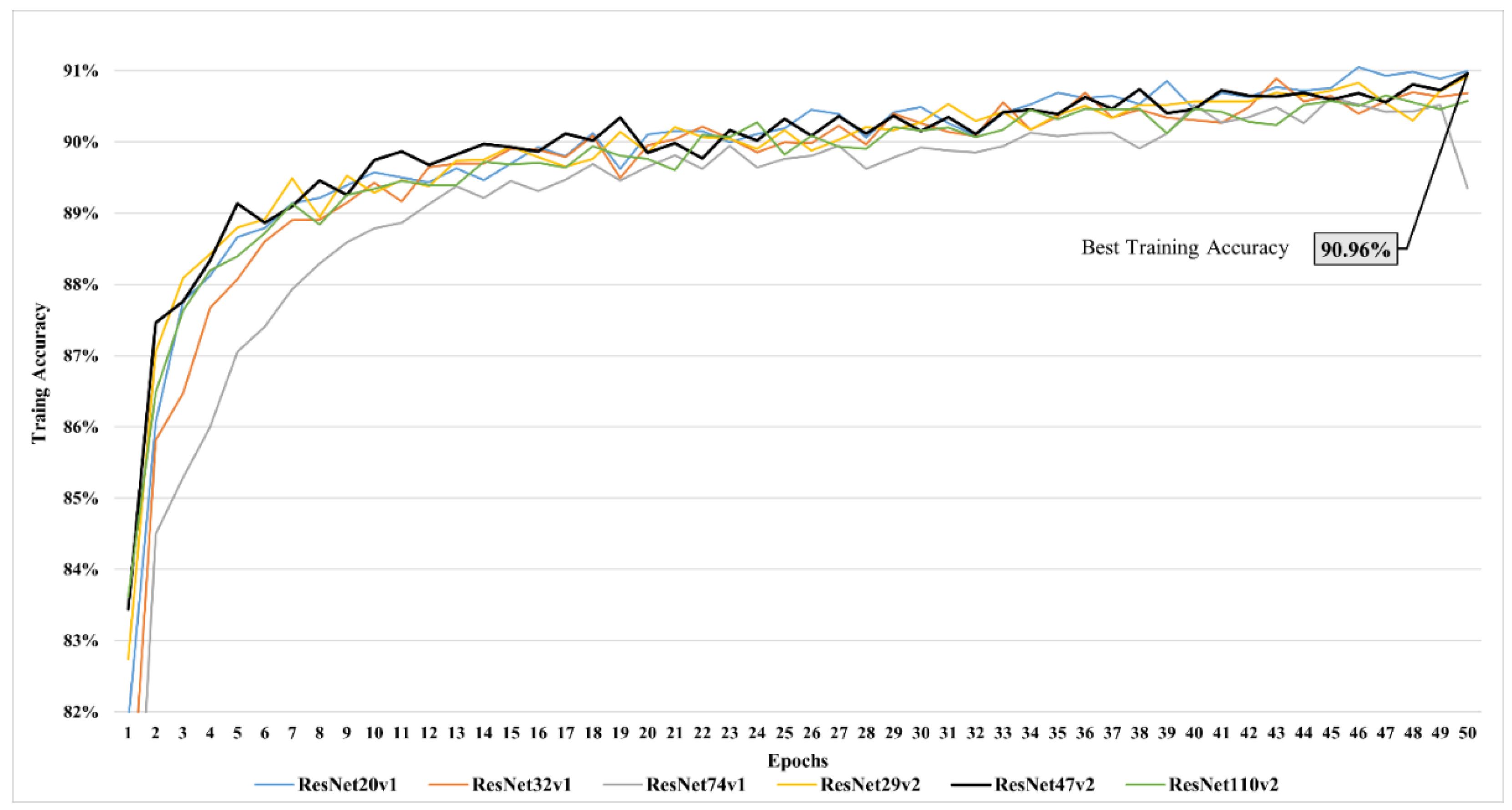
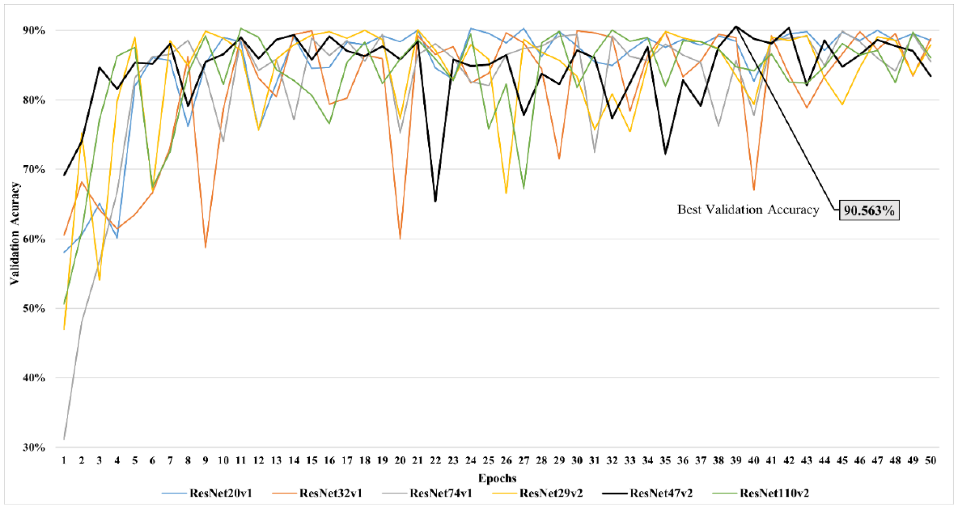
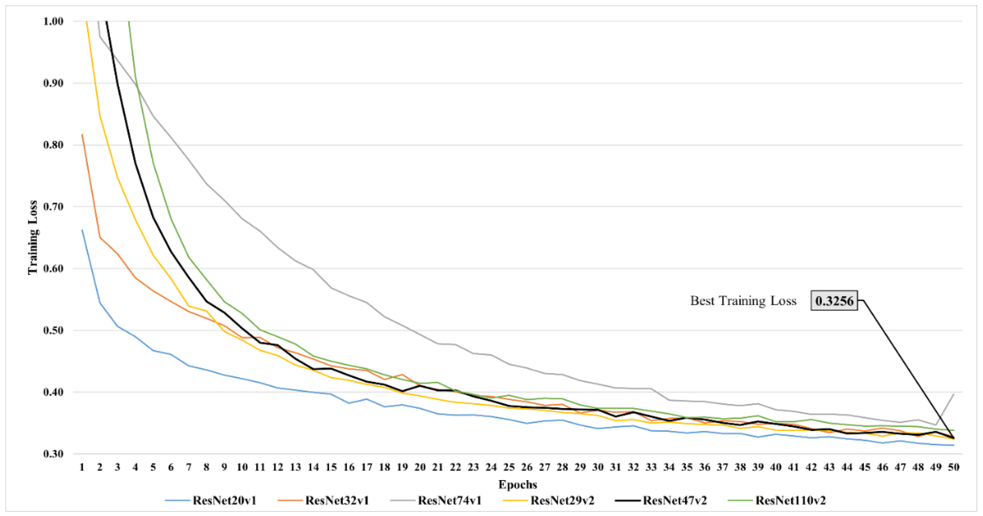
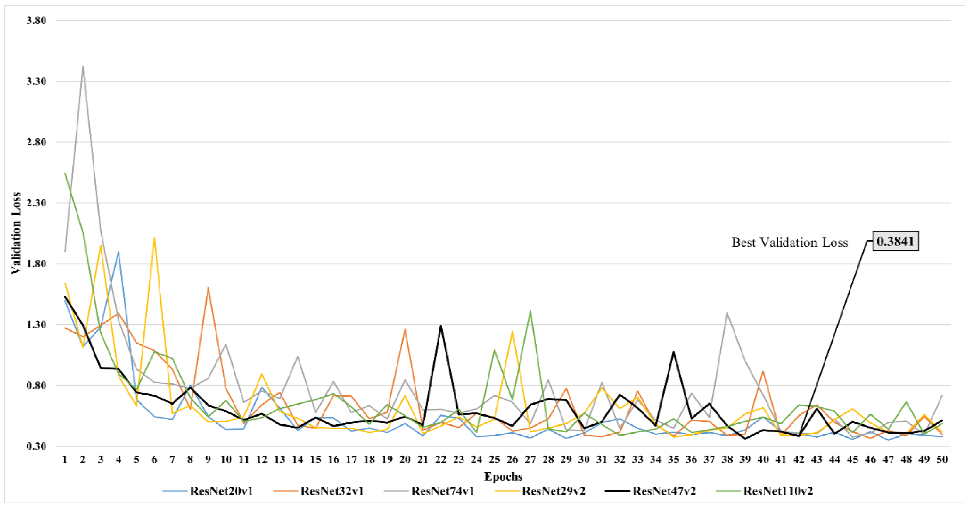
| Model | # of Layers | Training Loss | Validation Loss | Training Accuracy (%) | Validation Accuracy (%) | Training Time (h) | Validation Time (h) |
|---|---|---|---|---|---|---|---|
| ResNet 1 | 20 | 0.3219 | 0.3579 | 90.76 | 89.77 | 75.00 | 0.18 |
| ResNet 1 | 32 | 0.3418 | 0.3668 | 90.40 | 89.80 | 133.76 | 0.30 |
| ResNet 1 | 74 | 0.3586 | 0.3771 | 90.62 | 89.88 | 278.83 | 0.55 |
| ResNet 2 | 29 | 0.3491 | 0.3770 | 90.38 | 89.86 | 173.74 | 0.29 |
| ResNet 2 | 47 | 0.3523 | 0.3621 | 90.40 | 90.56 | 291.30 | 0.55 |
| ResNet 2 | 110 | 0.3738 | 0.3895 | 90.07 | 90.05 | 671.26 | 0.96 |
| Reference | Methodology | Accuracy (%) |
|---|---|---|
| This paper | Modified superpixel grains with ResNet2 with 47 layers | 90.56 |
| Julien et al. (2019) [22] | Superpixel color features with random forests | 89.00 |
| Julien et al. (2019) [22] | Superpixel segmented grains with CNN | 49.23 |
| Brian et al. (2021) [50] | Neighborhood component analysis and cubic SVM | 65.75 |
| Brian et al. (2021) [50] | Neighborhood component analysis quadratic SVM | 39.72% |
Publisher’s Note: MDPI stays neutral with regard to jurisdictional claims in published maps and institutional affiliations. |
© 2022 by the authors. Licensee MDPI, Basel, Switzerland. This article is an open access article distributed under the terms and conditions of the Creative Commons Attribution (CC BY) license (https://creativecommons.org/licenses/by/4.0/).
Share and Cite
Latif, G.; Bouchard, K.; Maitre, J.; Back, A.; Bédard, L.P. Deep-Learning-Based Automatic Mineral Grain Segmentation and Recognition. Minerals 2022, 12, 455. https://doi.org/10.3390/min12040455
Latif G, Bouchard K, Maitre J, Back A, Bédard LP. Deep-Learning-Based Automatic Mineral Grain Segmentation and Recognition. Minerals. 2022; 12(4):455. https://doi.org/10.3390/min12040455
Chicago/Turabian StyleLatif, Ghazanfar, Kévin Bouchard, Julien Maitre, Arnaud Back, and Léo Paul Bédard. 2022. "Deep-Learning-Based Automatic Mineral Grain Segmentation and Recognition" Minerals 12, no. 4: 455. https://doi.org/10.3390/min12040455