A Novel Enhanced Total Gradient (ETG) for Interpretation of Magnetic Data

Abstract

Edge detection techniques identify the horizontal extents of the underground geological bodies and work well in association with magnetic as well as seismic data. Even though the detected edges might not be a lithological contact, they offer first-hand information regarding various rocks that ultimately offers an extra argument for existing tectonics. Most of the edge enhancement techniques depend either on the horizontal gradient or total gradient of the potential fields. As of now, no single edge detection filter performance is best in all conditions. The study proposes a novel edge detection filter called “ETG-Enhanced Total Gradient” that combines the derivatives of the analytic signal (AS) (in the third dimension). The maximum amplitude of the AS is less dependent of the direction of magnetization and is critical in mapping the borders of the buried magnetic sources beneath the Earth. As the ETG filter is based on the total gradient of the field, there is no need to apply reduction to the pole process on the magnetic data. One limitation of the method is that the filter is unable to perform better at the corners where the other conventional methods miserably failed. The filter’s behavior is examined and validated using 2D and 3D synthetic magnetic data. The reliability of the ETG filter is examined by applying it to the magnetic data of the Seattle uplift region, USA. A new structural map of the region is generated by using the proposed ETG filter. The observed peak response of the ETG filter is well correlated with major tectonic features such as the Seattle Fault Zone (SFZ), Hood Canal Fault (HCF), and Dewatto Fault (DF).

1. Introduction

Edge detection is a fundamental operation in the geological interpretation constrained by magnetic field data [1]. The main principle in examining the geological contacts in the magnetic field is to determine the exact location and extents of the sources based on the measured magnetic properties of the rocks, such as magnetic susceptibility. Mapping the edges of various source rocks can group the lithologies of a similar magnetic field based on the detected edge along the contact of the two geological bodies. Even though the detected edges might not be a lithological contact, this offers first-hand information regarding various rocks and their geological domains that ultimately offers an extra argument for existing tectonic evolution. Numerous enhancement filters have been used to examine the boundaries of the sources buried at different depths on an observation plane [2,3,4]. These studies enhance the filter’s efficacy by delineating the true edges of the buried magnetic sources [5,6]. It is quite interesting to note that the edge enhancement techniques are successfully used to map the boundary of the salt dome in seismic image interpretation [7,8]. It is worth mentioning that enhancements in the edge detection filters are sensitive to factors like (i) accuracy in delineated edges, (ii) crossed interfaces, (iii) balancing the signal sources present at various depths, (iv) direction of magnetization, (v) dip of the interface, (vi) sensitivity to noise and (vii) capability of working over bodies with thin dimensions and less susceptibility contrast [9,10,11,12]. Most of the edge detection techniques are unable to recover the true edge of the buried bodies with dip and non-vertical magnetic fields. When the data is vertically magnetized, the edge detection filter task is straightforward. However, in the real Earth case, it is obvious that the magnetization of the different rocks could be vertical as well as non-vertical.

2. Previous Edge Detection Studies

Edge detection is the most common interpretation technique applied to gravity and magnetic data for delineating the subsurface bodies with contrasting susceptibility or density. Several edge detection techniques utilize the first, second, or even third-order derivatives of the magnetic field to delineate the susceptibility contrasting zones [11,12]. Several methods are in use for interpreting the size and shape factors of the causative bodies. Several studies have proposed filters on magnetic data to delineate the geological domain boundaries, faults, lineaments and shear zones.

Table 1. Previous edge detection techniques. Abbreviations are used in the table for reducing the column size and are listed as follows: HG: Horizontal Gradient; AS: Analytic Signal; TA: Tilt angle; HGTA: Horizontal gradient of tilt angle; TM: Theta map; TDX: Normalized horizontal tilt; HTA: Hyperbolic tilt angle; TAHG: Tilt angle of the horizontal gradient; TBHG: Tilt angle of the balanced horizontal gradient; TAAS: Tilt angle of the analytic signal.

Method (Reference)	Quantity Related to Edge	Advantages	Limitations
$HG=\sqrt{{\left(\frac{\partial M}{\partial x}\right)}^2+{\left(\frac{\partial M}{\partial y}\right)}^2}$ [13]	Maximum	1. Less sensitive to noise.	1. Poor performance in balancing the signals from shallow and deep anomalies. 2. Require magnetic reduction-to-the-pole
$\left|AS\right|=\sqrt{{\left(\frac{\partial M}{\partial x}\right)}^2+{\left(\frac{\partial M}{\partial y}\right)}^2+{\left(\frac{\partial M}{\partial z}\right)}^2}$ [14]	Maximum	1. Less dependent on the direction of the magnetization vector	1. Poor performance in balancing the signals from shallow and deep anomalies.
$TA={tan}^{-1}\left(\frac{\frac{\partial M}{\partial z}}{\sqrt{{\left(\frac{\partial M}{\partial x}\right)}^2+{\left(\frac{\partial M}{\partial y}\right)}^2}}\right)$ [15]	Zero	1. Can generate a balanced image for the sources situated at different depths.	1. Require magnetic reduction-to-the-pole. 2. Produces secondary edges around the true edge.
$HGTA=\sqrt{{\left(\frac{\partial TA}{\partial x}\right)}^2+{\left(\frac{\partial TA}{\partial y}\right)}^2}$ [16]	Maximum	1. The method enhances the maximum horizontal gradients in low wavelength anomalies.	1. Require magnetic reduction-to-the-pole. 2. Produces secondary edges around the true edge.
$TM={cos}^{-1}\left(\frac{\sqrt{{\left(\frac{\partial M}{\partial x}\right)}^2+{\left(\frac{\partial M}{\partial y}\right)}^2}}{\sqrt{{\left(\frac{\partial M}{\partial x}\right)}^2+{\left(\frac{\partial M}{\partial y}\right)}^2+{\left(\frac{\partial M}{\partial z}\right)}^2}}\right)$ [17]	Minimum	1. The TM filter produces balances between edges located at different source depths.	1. Require magnetic reduction-to-the-pole. 2. Produces secondary edges around the true edge.
$TDX={tan}^{-1}\left(\frac{\sqrt{{\left(\frac{\partial M}{\partial x}\right)}^2+{\left(\frac{\partial M}{\partial y}\right)}^2}}{\left|\frac{\partial M}{\partial z}\right|}\right)$ [18]	Maximum	1. Can generate a balanced image for the sources situated at different depths.	1. Require magnetic reduction-to-the-pole 2. Produces secondary edges around the true edge
$HTA=ℛ\left({tanh}^{-1}\left(\frac{\frac{\partial M}{\partial z}}{\sqrt{{\left(\frac{\partial M}{\partial x}\right)}^2+{\left(\frac{\partial M}{\partial y}\right)}^2}}\right)\right)$ [18]	Maximum	1. Can generate a balanced image for the sources situated at different depths.	1. Require magnetic reduction-to-the-pole 2. Produces secondary edges around the true edge.
$TAHG={tan}^{-1}\left(\frac{\frac{\partial \left(HG\right)}{\partial z}}{\sqrt{{\left(\frac{\partial \left(HG\right)}{\partial x}\right)}^2+{\left(\frac{\partial \left(HG\right)}{\partial y}\right)}^2}}\right)$ [19]	Maximum	1. Can generate a balanced image for the sources situated at different depths.	1. Detected edges have low resolution. 2. Require magnetic reduction-to-the-pole
$TBHG={tan}^{-1}\left(\frac{\frac{\partial B}{\partial z}}{\sqrt{{\left(\frac{\partial B}{\partial x}\right)}^2+{\left(\frac{\partial B}{\partial y}\right)}^2}}\right)$ where $B=\left(\frac{HG}{k+\sqrt{H_x\left(HG\right)+H_y\left(HG\right)+H{G}^2}}\right)$ [20]	Maximum	1. Can generate a balanced image for the sources situated at different depths.	1. Detected edges have low resolution. 2. Require magnetic reduction-to-the-pole
$TAAS={tan}^{-1}\left(\frac{\frac{\partial AS}{\partial z}}{{\left(\frac{\partial AS}{\partial x}\right)}^2+{\left(\frac{\partial AS}{\partial y}\right)}^2}\right)$ [21]	Maximum	1. Perform is same on the datasets situated at different latitudes.	1. Detected edges have low resolution.

lists the previous edge detection techniques used in the present research work for a comparative study that includes the technique’s formula, used for computing the source edges, defined edge value from the response, and potential advantages and limitations.

3. Proposed Method

The maximum amplitude of the AS (in the third dimension) is independent of the direction of magnetization and is critical in mapping the borders of the buried magnetic sources beneath the Earth. The AS filter peaks just over the edges of the magnetic source [14,22,23]. Nevertheless, the amplitudes are blurred if the bodies are buried at a deeper depth, and the shallow-seated bodies dominate the AS amplitude [11,12,14,23,24,25]. Even though the filter works independently of the directions of magnetization and ambient magnetic field, the blurriness caused by the response of the deep-seated magnetic sources makes this filter unworthy for geological interpretation. This situation calls for the AS method to enhance the response from the deep-seated anomalies that further generate a balanced image of the buried sources. The second-order vertical derivatives of the analytic signal are utilized to design the Enhanced Total gradient (ETG) function and are defined in Equation (1).

$$ETG=0.5\times \left({\tan }^{-1}\left(\frac{\left(A{S}_{zz}\right)-\left(\sqrt{{\left(A{S}_{zx}\right)}^2+{\left(A{S}_{zy}\right)}^2}\right)}{\left|A{S}_{zz}\right|}\right)+{\tan }^{-1}\left(\frac{\left(A{S}_{zz}\right)-\left(\sqrt{{\left(A{S}_{zx}\right)}^2+{\left(A{S}_{zy}\right)}^2}\right)}{\left|\sqrt{{\left(A{S}_{zx}\right)}^2+{\left(A{S}_{zy}\right)}^2}\right|}\right)\right)$$

(1)

Here $A{S}_{zz}$ is assumed to be a negative summation of the second derivative of AS in x- and y-directions as $A{S}_{zz}=-\left(A{S}_{xx}+A{S}_{yy}\right)$, which is used to localize the edges with zero-crossings of the high-frequency components in the magnetic field response [26].

As the ETG filter is based on the total gradient of the magnetic field, it can complement the reduction to the pole process. As defined by [27], the absolute value of the AS is described as the energy envelope of the field that is maximum over the contrasting magnetic zones. This eventually states that the amplitudes of the AS-dependent ETG filter peak directly over the center of the buried source edge. Even though the ETG filter is developed on the third-derivatives of the data, the resolution in the response of the filter is not compromised and performs as good as [21,28]. This can further be demonstrated in detail in the ensuing section.

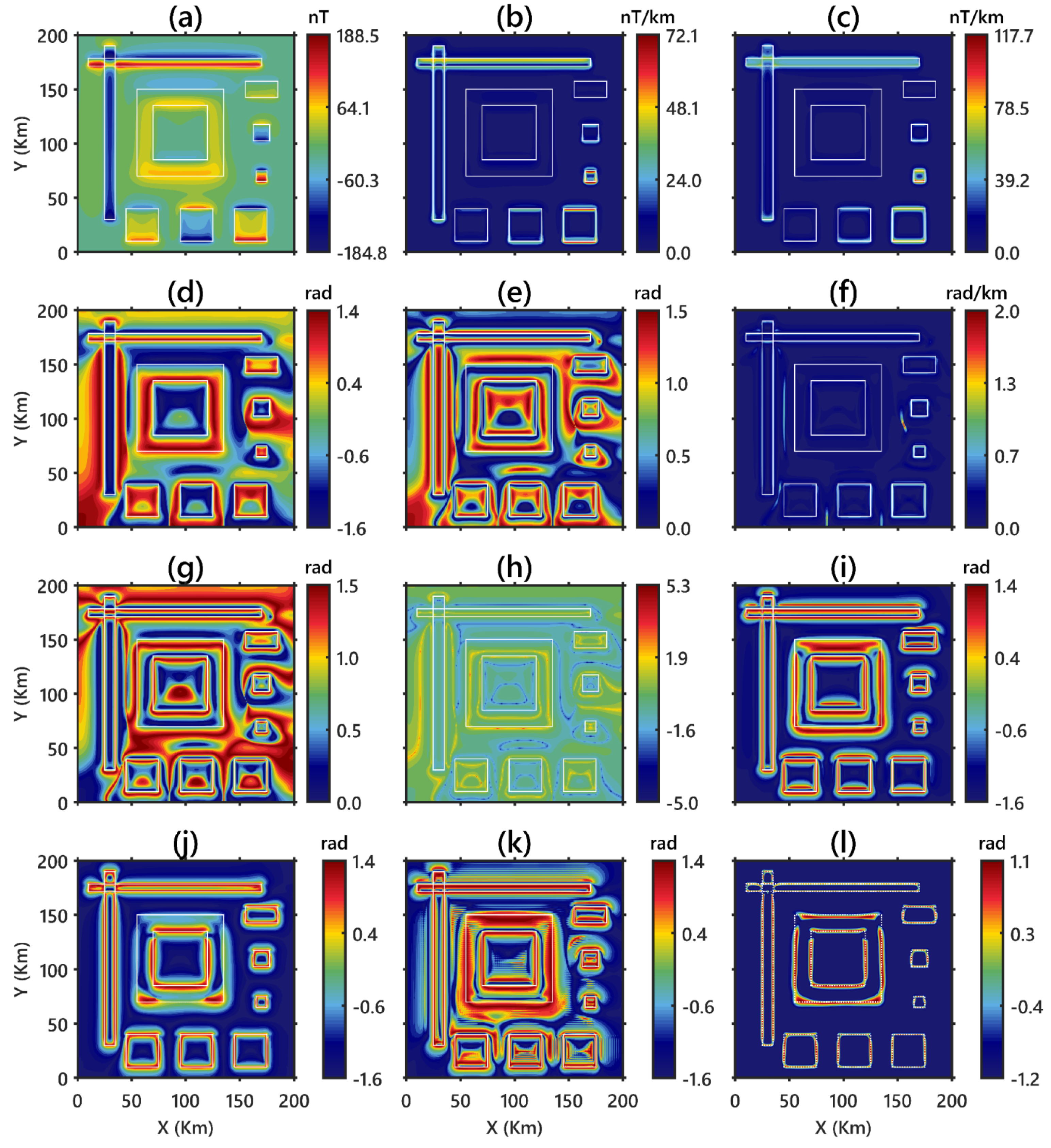
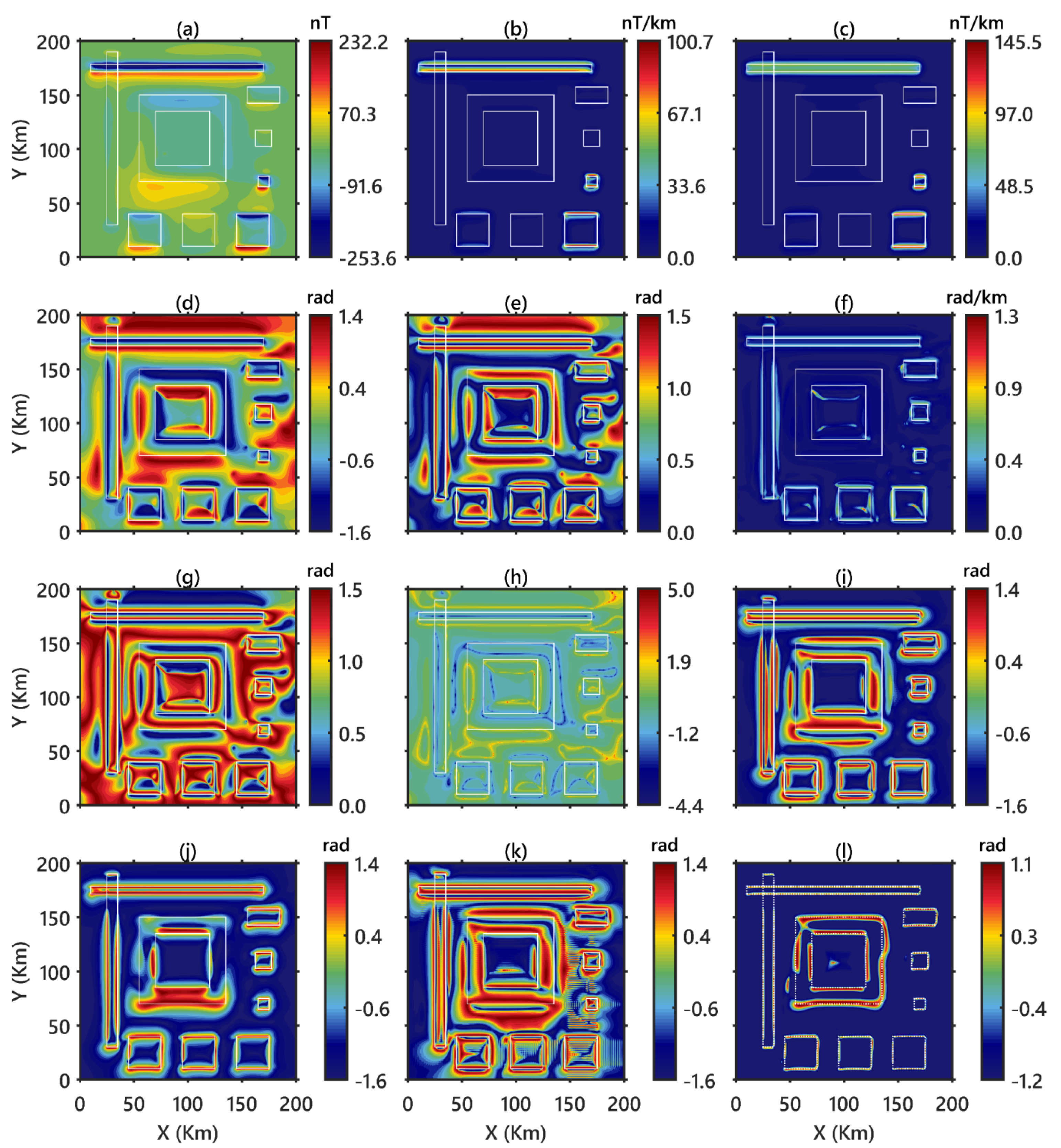
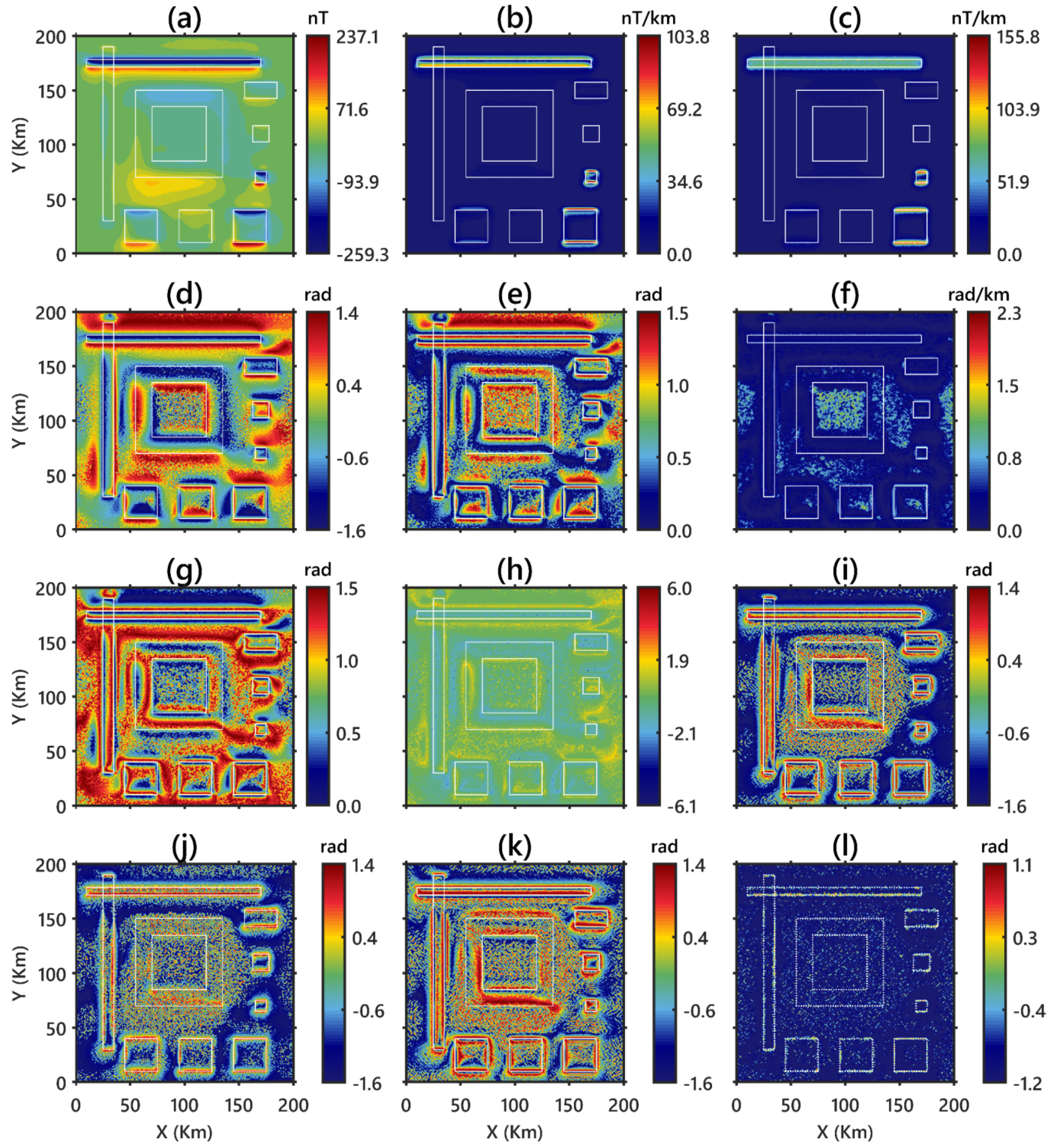
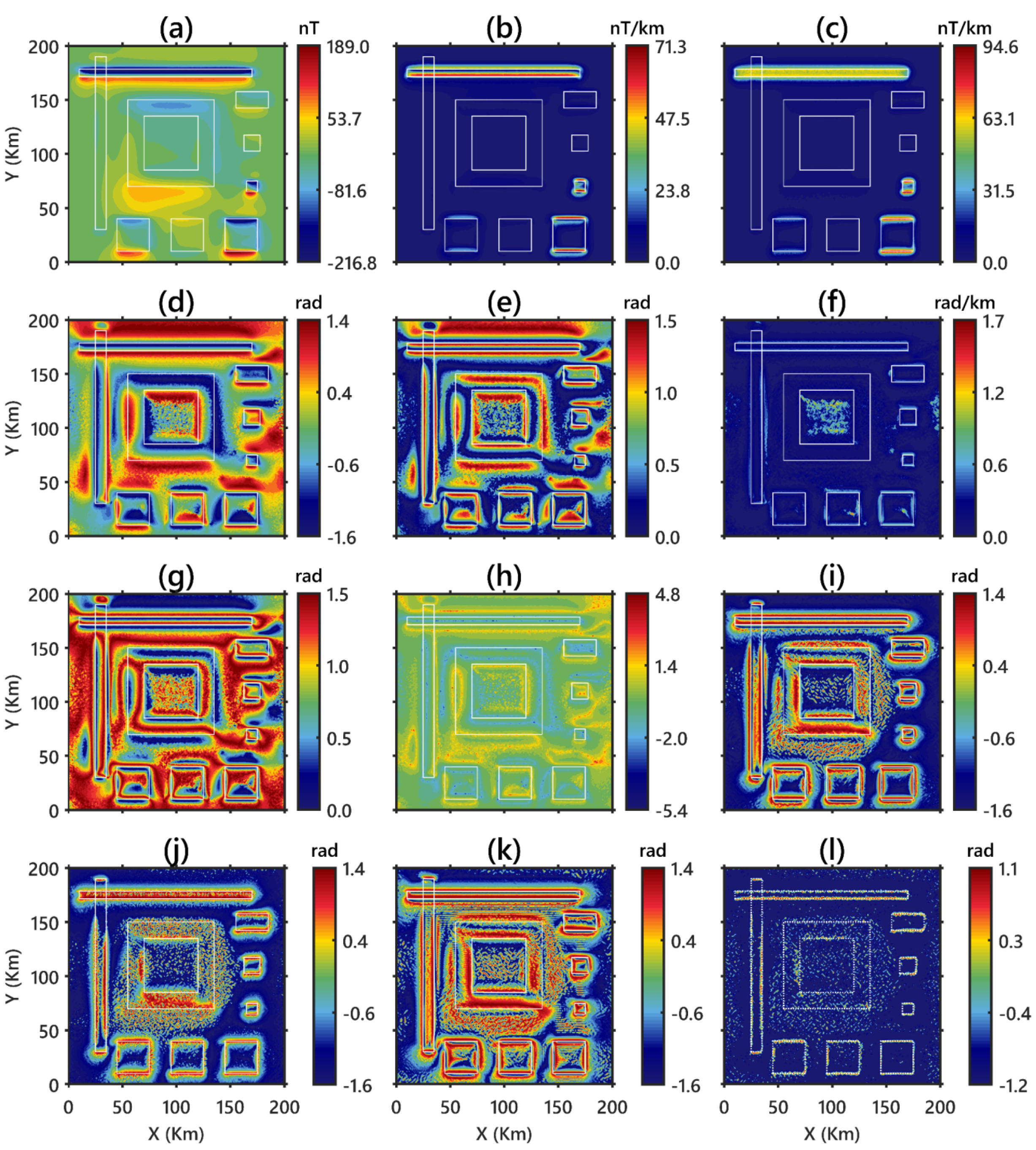
4. Validating the Response of the ETG Filter

Two special cases are introduced in the present work to validate the results obtained from the ETG filter. They are the responses over (i) 2D dipping dyke, (ii) 3D synthetic magnetic anomalies using a complex model constructed with ten prisms. The results are compared with the conventional edge detection filters which are listed in Table 1.

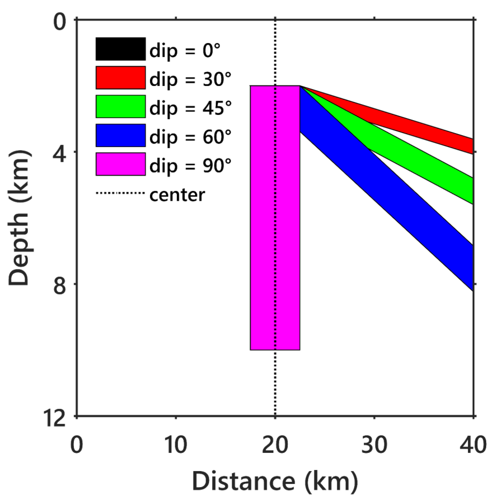
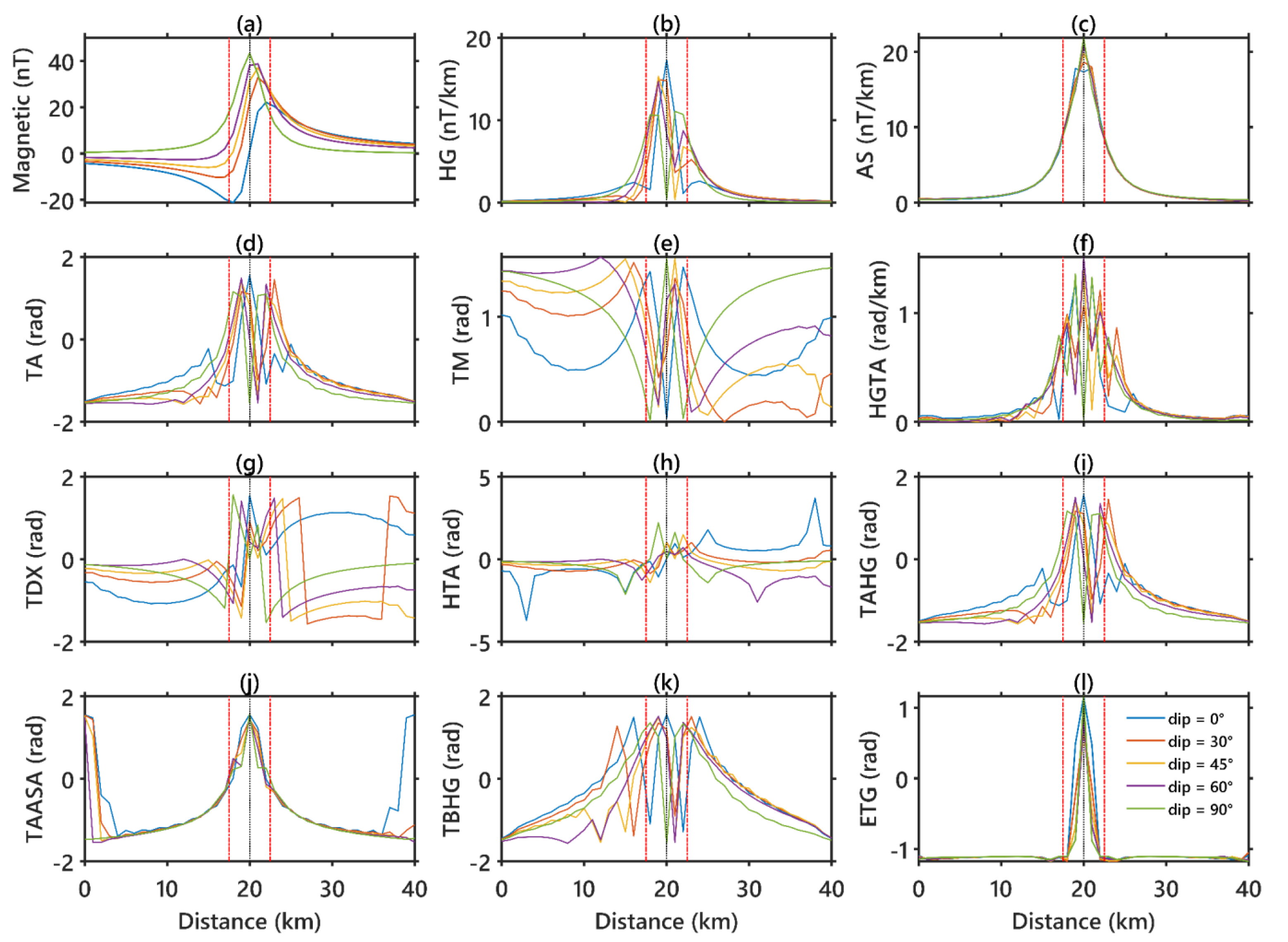
4.1. ETG Response over 2D Dipping Dyke

A simple 2D model is considered for the evaluation of the proposed ETG filter for validating its response over a buried dyke mode dipped at 0°, 30°, 45°, 60° and 90°. The dyke body has a width and height of 5 and 8 km, respectively. The dyke is buried at a depth of 2 km below the surface. The schematic diagram of the dipping dyke model at different dips is presented in Figure 1, and the magnetic anomaly response over the dipping dyke is shown in Figure 2a. The response of the edge detection methods, namely HG (Figure 2b), AS (Figure 2c), TA (Figure 2d), TM (Figure 2e), HGTA (Figure 2f), TDX (Figure 2g), HTA (Figure 2h), TAHG (Figure 2i), TAAS (Figure 2j) and TBHG (Figure 2k), represents that a change in the dip of the buried body obviously changes the response of the edge detection filters. It is clear from Figure 2 that, except for the filters that are developed using the total gradient of the field, the rest of the filters failed to extract the edge of the buried source. The performance of the two filters, AS (Figure 2c) and TAAS (Figure 2j), proves that, even though the dip of the dyke is changed, the filters continue to perform better. The response of the AS is sharp and peaks at the center of the body when the dip of the dyke is 90°, and the peak position is shifted away from the center when the dip approaches 0°, where a double-peak response is observed (Figure 2c) that is a limitation of the AS amplitude. The TAAS performed better than AS when dip = 0°, but the spurious maxima observed at either end of the response can lead to a false interpretation of the unknown sources (Figure 2j). The maximum amplitude of the ETG method is directly peaks over the center of the body (Figure 2l). The minimum amplitude is directed away from the center of the body and does not correspond to any geological contact. The maximum amplitude of ~1.1 radians is observed over the center of the body. There are no spurious peaks observed in the 2D response of the ETG function. The ETG filter performed similarly in all the cases when the dip of the dyke is changed between 0° and 90°. This is the advantage of the ETG over all the other conventional filters compared in the present study. In addition, even though the direction of magnetization of the field is changed, the response of the ETG filter remained the same.

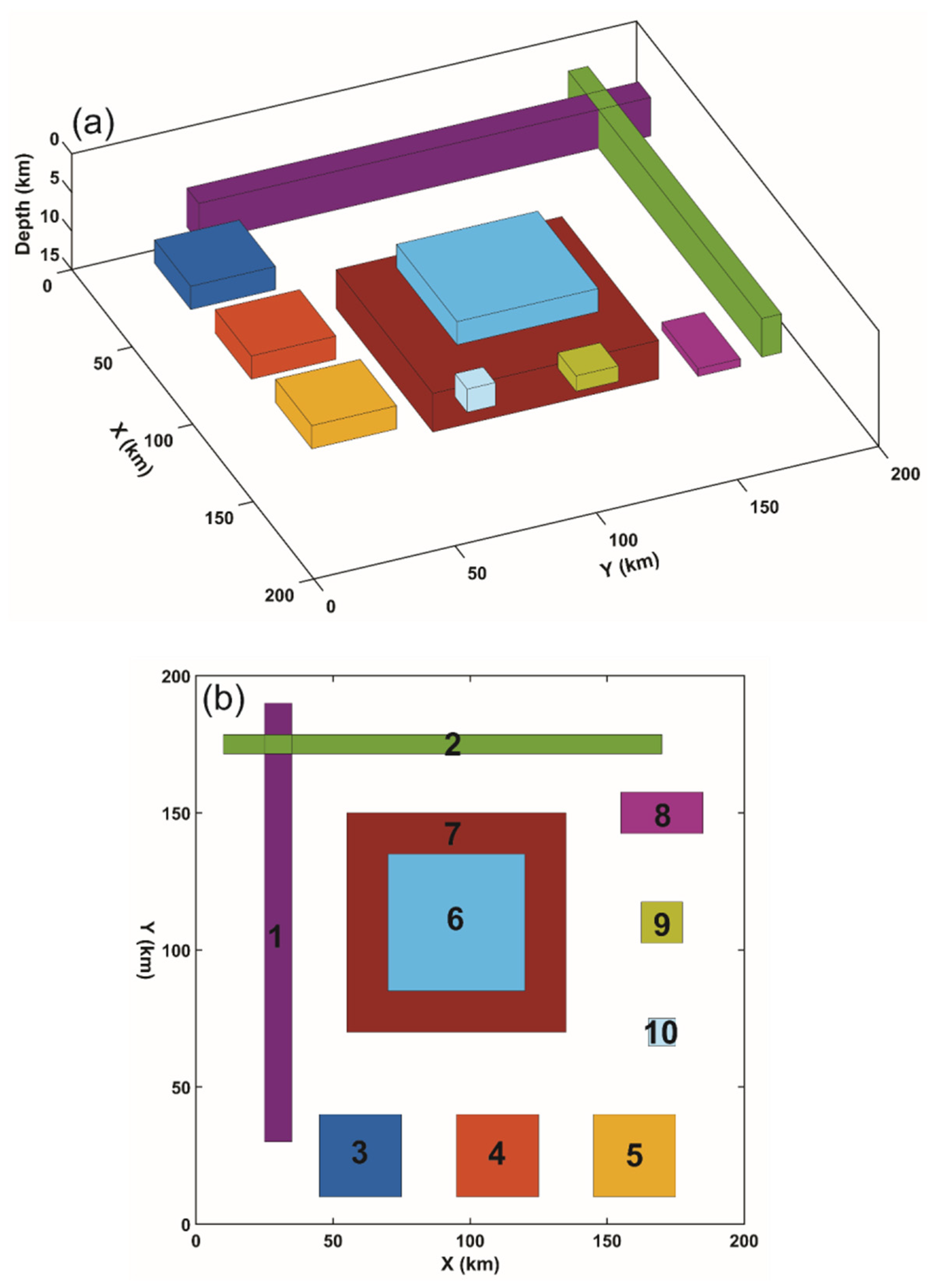
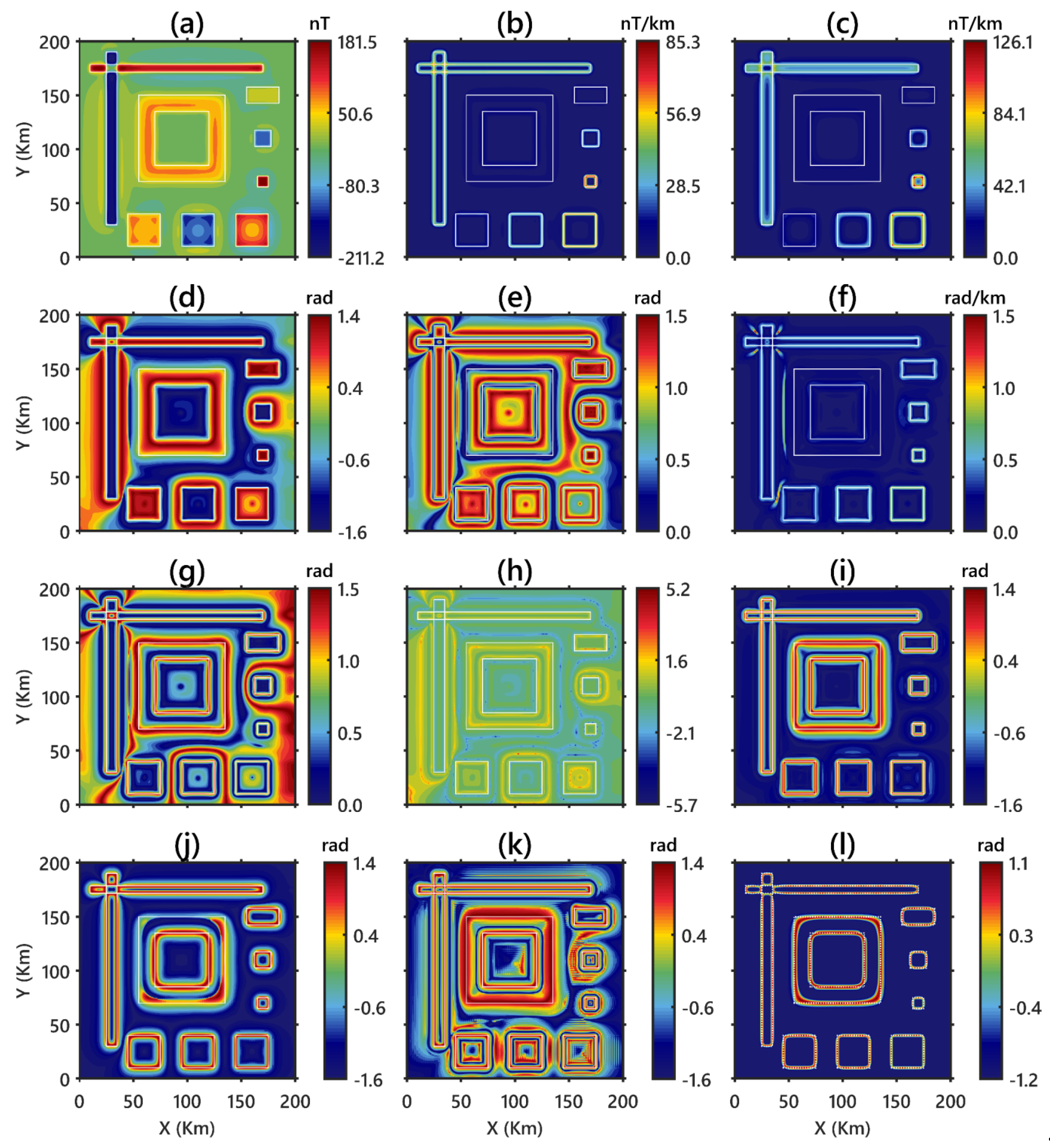
4.2. ETG Response over 3D Magnetic Sources

The efficacy of the ETG technique is illustrated by application over the 3D synthetic magnetic data consisting of ten prisms, each with different dimensions and physical properties. The schematic diagram of the 3D synthetic model considered for the present study is shown in Figure 3a, and the nomenclature with 2D representation is presented in Figure 3b. The dimensions and physical properties of the ten prismatic sources are listed in

Table 2. Geometry and magnetization parameters of the 3D synthetic model.

Parameter	P1	P2	P3	P4	P5	P6	P7	P8	P9	P10
X-center (km)	30	90	60	110	160	95	95	170	170	170
Y-center (km)	110	175	25	25	25	110	110	150	110	70
Width (km)	10	160	30	30	30	50	80	30	15	10
Height (km)	160	7	30	30	30	50	80	15	15	10
Top Depth (km)	2	2	3	2	1	5	10	3	2	1
Thickness (km)	5	5	3	3	3	3	5	1	2	3
Susceptibility (SI)	−0.02	0.02	0.02	−0.021	0.02	−0.026	0.028	0.023	−0.021	0.022

. The total magnetic intensity of the model is set to 44,500 nT (as per the IGRF model). The anomaly due to the 3D prismatic model is calculated with a 1 km sampling interval at 201 × 201 grid nodes. Here, four important cases were considered: (1) The azimuth, inclination and declination of the field are set to 0°, 90° and 0° for all the sources, respectively; (2) The azimuth, inclination and declination of the field are set to 0°, 33° and 0.19° for all the sources (magnetic field parameters of central Indian tectonic zone as per IGRF model), respectively; (3) The remanent magnetization direction is (Ir, Dr) = (10°, 25°), and a remnant magnetization of 0.5 is introduced to all the model’s bodies of the second case; (4) 4% Gaussian noise added to the magnetic anomaly of the third case.

The magnetic anomaly in the first case is represented in Figure 4a. Figure 4b–l show the results of the HG, AS, TA, TM, HGTA, TDX, HTA, TAHG, TAAS, TBHG, and ETG methods, respectively. We can see that the HG, AS, and HGTA filters cannot be applicable to outline the borders of the deeper bodies and hence fail to balance the amplitudes from the sources at different depths [11,12,22,28]. The TA, TM, TDX, and HTA methods produce numerous spurious anomalies around the true edges of the bodies making the interpretation complicated, which [29,30] also observed. The TAHG filter is effective in delineating all the borders. Like TAHG, the filter TAAS is effective in delineating all the borders, but its performance does not seem to perform well over bodies with superimposed magnetic source bodies (P6 and P7). The TBHG filter can delineate all the borders, but it also produces numerous spurious edges. The proposed ETG filter is successful in delineating the edges of all the buried magnetic sources with better accuracy than the above discussed conventional edge detection filters. No false edges are produced in the filtered response of the ETG filter.

In the second case, the magnetic anomaly response of the model is represented in Figure 5a. In this case, it is observed that, when the parameters of the model are close to the real data parameters, all the methods (Figure 5b–k) failed to identify a clear picture of the true edges of the subsurface bodies. Amongst the conventional filters tested in the present study, TAHG’s (Figure 5i) performance is comparatively better, but the horizontal edges have been found with false edges and are not clearly visible. The ETG filter response (Figure 5l) is outstanding when compared to the other methods. The proposed method clearly identified the source edges, irrespective of the sign of magnetic susceptibility, magnetic inclination and declination. One limitation of the method is that the filter is unable to perform better at the corners, where the other methods miserably failed.

The magnetic anomaly in the case of the remanent magnetization induced to the model is represented in Figure 6a. Similar to the second scenario, all the filters failed to outline the source, including TAHG (Figure 6b–k). The proposed ETG filter is effective in delineating all the borders except the body with superimposed anomalies (P7) (Figure 6l). P7 is situated at 10 km depth, and with the influence of remnant magnetization the edge of the prismatic body is not linear.

In the fourth case, 4% Gaussian noise added to the magnetic anomaly of the third case (Figure 7a). Almost all the conventional filters (Figure 7b–k) failed to highlight the borders under the influence of noise in the data. Similar to the other conventional methods based on total gradient, the performance of the ETG filter (Figure 7l) is rather poor and is the limitation of the proposed filter. In order to overcome this limitation, one solution is to continue the magnetic anomaly to a certain height that is based on the interpreter. Likewise, we opted for 1000 m as continuation height to visualize the performance of the filters (Figure 8a). We observed that, when the magnetic response continued to 1000 m, the ETG filter performed better than other conventional filters (Figure 8b–k), delineating all the edges of the magnetic sources except the superimposed bodies (Figure 8l).

5. Application of ETG over Aeromagnetic Data of Seattle Uplift (SU), USA

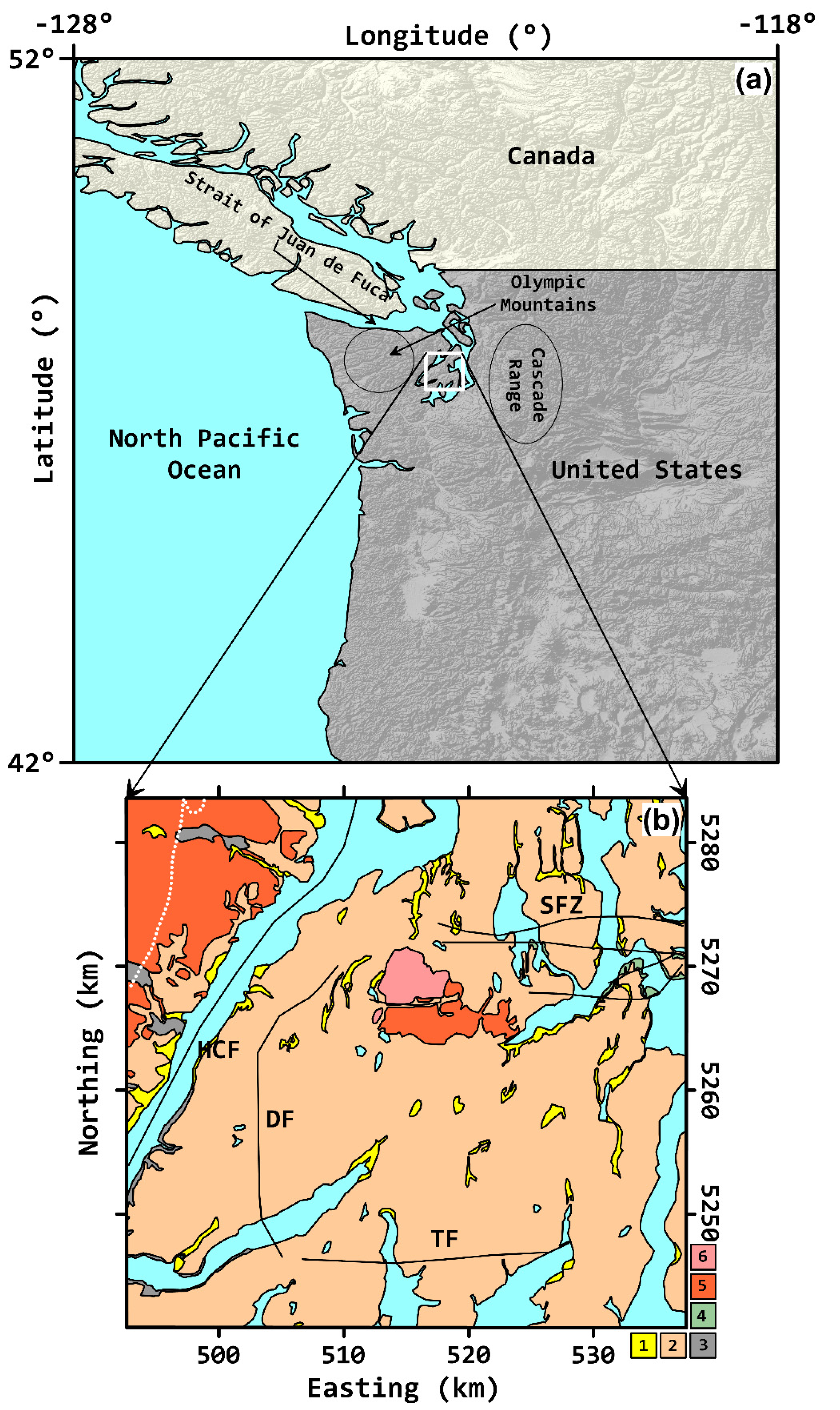
5.1. Study Region

The aeromagnetic anomaly over the Seattle Uplift, USA, is used to represent the practical utility of the proposed ETG filter. The location of the study region is shown in Figure 9a and the geology of the region [29,31] with the major tectonics is represented in Figure 9b. The study region is bounded by the North Pacific Ocean and the Olympic Mountains in the west, Strait of Juan de Fuca in the north-west and the Cascade Range in the east. The subduction setting of the Juan de Fuca plate under the North American continent created an unstable tectonic condition and resulted in the northeast migration of the coastal regions of Washington and surrounding regions. The migration is counter attacked by the stable cratonic blocks of the southwest Canadian region resulting in the activation of numerous fault zones between major tectonic settings of the Seattle uplift region [32,33,34]. The Crescent formations present in the northwest corner of the study region are divided into the Lower and Upper member basalt, where a solid white dotted line is represented in Figure 9a for division.

There are several active tectonic faults present in the region, namely Seattle Fault Zone (SFZ), Hood Canal Fault (HCF), Tacoma Fault (TF) and Dewatto Fault (DF) [31]. The Seattle fault is reflected as a crustal fault in the study region that hosted a large Holocene earthquake and can better be called as Seattle Fault Zone (SFZ) because of its huge width (5–7 km) with numerous faults and deformed shallow strata ([35] and references therein). The HCF is a NE-SW trending linear-natured strike-slip fault beneath Hood Canal, which probably transfers strain onto the SFZ as suggested by [36]. The TF is a steep north dipping buried reverse fault where the northern side of the fault is uplifted, and its eastern end comprises numerous lineaments along a 10 km wide zone [37]. The DF is present on the western end of the Seattle uplift region and exhibits two different trends, being north directed in its southern end and NW-SE directed in its southern tip. According to [34], DF is thought to be initiated with the exhumation of the Olympic Massif. The Seattle uplift is thought to be controlled by two nearly orthogonal faults (TF and DF) bounding it in the southern and western corners.

5.2. Aeromagnetic Data

The high-resolution aeromagnetic data (Figure 10a) were acquired by the U.S. Geological Survey department during the late 1990s with north-south directed flight lines, a flying height of 250 m and a 400 m sampling interval [38]. The amplitudes of the magnetic anomalies in the study region varies between a minimum of ~−620 nT to the north of SFZ and a maximum of ~1018 nT that surrounds the Seattle uplift region. The low amplitude of the magnetic anomaly dominates the study region that covers the southwest of the DF and eastern end of the TF. The high amplitude magnetic anomalies are present at the center of the map over the Seattle uplift region. The SFZ is governed by low amplitude magnetic anomalies, whereas the HCF divides the moderate NE-SW trending elongated magnetic anomalies in the east from the low amplitude anomalies to its west. In order to remove the effect of erroneous near-surface magnetic sources, the magnetic anomaly is continued to 200 m upward (Figure 10b). The upward continued magnetic anomaly is used to extract the pseudo-structural magnetic fabric of the study region, and the amplitude varies between ~−560 to 865 nT (Figure 10b).

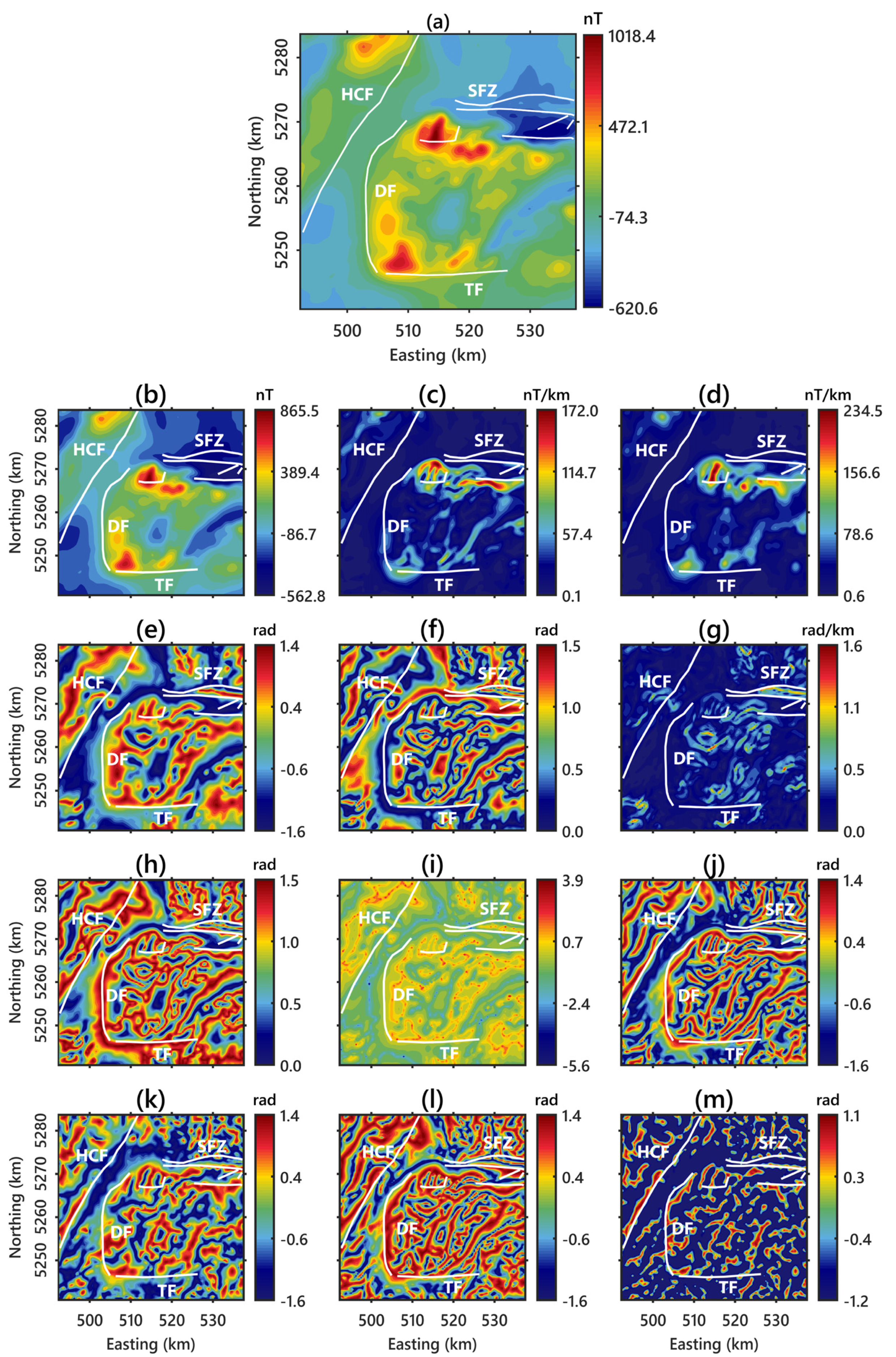
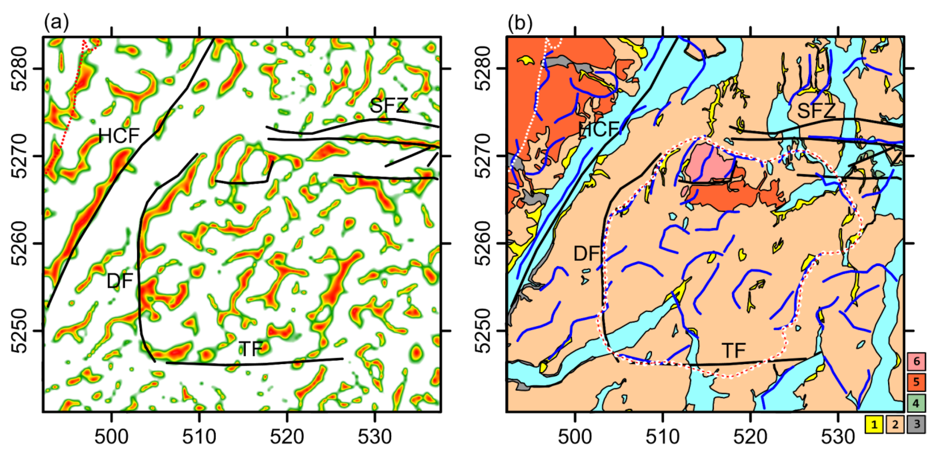
5.3. Results and Discussion

The magnetic anomaly, which continued to 200 m upwards (Figure 10b), is used to map the subsurface structures. The subsurface structures identified by various edge detection techniques are shown in Figure 10c–l. The edges obtained from the ETG method are displayed in Figure 10m, superimposed by the major tectonic features [31,34]. The magnetic analysis shows that both HG (Figure 10c) and AS (Figure 10d) are dominated by the large anomalies from the southern margin of the SFZ. Both AS and HG are good at deciphering the linear structures that are present at a shallower depth, unable to balance the linear features, and unable to produce a signal from the deep subsurface geological structures [11]. The phase-based filters like TA (Figure 10e), TBHG (Figure 10l) and TM (Figure 10f) were successful in delineating the magnetic lineaments. However, the detected edges are not sharp enough for visual inspection. The HGTA map is shown in Figure 10g. As stated in scenario 1, the filter is unable to balance the borders of the bodies with sources at different depths, which is an inherent quality of a filter designed based on horizontal gradient.

The TDX and HTA filters (Figure 10h,i, respectively) are successful in detecting the horizontal extents of most of the geological boundaries. Nonetheless, false boundaries were determined, and many adjacent edges were found to be interconnected in the response of HTA. The synthetic scenarios suggest that the delineated edges have a considerable shift from the true geological boundary. The filters TAAS (Figure 10k) and TAHG (Figure 10j) are successful in identifying the geological contacts. Amongst the applied edge enhancement filters applied to the aeromagnetic data over the Seattle uplift region, the filters based on the HG and its derivatives need the reduction to pole process so we can observe a shift of linear features. However, the filters AS, TAAS and ETG (Figure 10m) have an exemption from the reduction to pole process, as they use the total gradient of the magnetic anomaly.

Figure 10. (a) The aeromagnetic anomaly map of the study region. The aeromagnetic anomaly map after continuing to 200 m upward is presented in (b). The response of various conventional edge detection filters namely (c) HG; (d) AS; (e) TA; (f) TM; (g) HGTA; (h) TDX; (i) HTA; (j) TAHG; (k) TAAS; (l) TBHG; and (m) ETG. The white lines over the response on all the figures show the true edge of the prisms.

Figure 10. (a) The aeromagnetic anomaly map of the study region. The aeromagnetic anomaly map after continuing to 200 m upward is presented in (b). The response of various conventional edge detection filters namely (c) HG; (d) AS; (e) TA; (f) TM; (g) HGTA; (h) TDX; (i) HTA; (j) TAHG; (k) TAAS; (l) TBHG; and (m) ETG. The white lines over the response on all the figures show the true edge of the prisms.

The proposed ETG technique is successful in delineating the boundaries of most of the geological contacts visible on the surface as well as buried under the top geological cover. A new structural map of the Seattle uplift region is interpreted from the response of ETG and is shown in Figure 11a, and the geology is overlaid on the existing and interpreted lineaments as shown in Figure 11b. Three types of gradients are generated in the magnetic analysis map (Figure 11a), out of which the magnetic gradients observed beneath the SFZ are aligned in E-W direction, the trends to the north are aligned, and the rest are mostly trending in NE-SW direction. It is clear that the contact between the upper and lower members of the Crescent Formations is identified reasonably well. Our analysis shows that the HCF has well-documented evidence in the magnetic gradient aligned in the NE-SW direction along its length. The magnetic gradient is continuous at its southern end but is discontinuous in its upper portion. However, we observed no seismic evidence to support the existence of a fault beneath Hood Canal [39]. The Seattle uplift zone is marked with a boundary based on the aligning trends at the outer edge of the Seattle uplift region (Figure 11b). The DF fault is represented by the peaks of the ETG filter and is consistent with its NE-SW trending nature at its northern end to ~N-S at its center and is interrupted by the NE-SW trending faults to its south-western margin. We were unable to detect any continuous ETG response beneath the TF. The structural map prepared using ETG response revealed numerous magnetic lineaments in the Seattle uplift region that were not recognized from the geologic map alone.

6. Conclusions

We introduced a new edge enhancement technique called “Enhanced Total Gradient” for outlining the boundaries of the subsurface bodies. The effectiveness of the ETG method is discussed over the magnetic anomaly generated on a dipping dyke model and a complex synthetic magnetic model and compared with performing conventional edge detection techniques. The main advantage of the ETG technique is that it reduces the filter dependency on the direction of magnetization. The results obtained from the model studies show that the ETG method can outline all the boundaries with no false information generated around the true boundaries. The method appears to effectively equalize the signal arising from the shallow and deep bodies. Under the influence of remnant magnetization, the technique performs better than other techniques. Since the ETG filter is developed on the third-derivatives of the data, the interpreter needs to apply the upward continuation technique to overcome the noise limitation of the ETG filter. The reliability of the ETG filter is also validated by applying it to the aeromagnetic data of the Seattle uplift region, USA. A new structural map is generated by using an ETG filter. The filter seems to perform better when compared to other techniques. The observed peak response of the ETG filter is well correlated with major tectonic features like HCF, DF and SFZ.

References

1. Eldosouky, A.M.; Abdelkareem, M.; Elkhateeb, S.O. Integration of remote sensing and aero-magnetic data for mapping structural features and hydrothermal alteration zones in Wadi Allaqi area, South Eastern Desert of Egypt. J. Afr. Earth Sci. 2017, 130, 28–37. [Google Scholar] [CrossRef]
2. Hang, N.T.; Thanh, D.D.; Minh, L.H. Application of directional derivative method to determine boundary of magnetic sources by total magnetic anomalies. Vietnam J. Earth Sci. 2017, 39, 360–375. [Google Scholar] [CrossRef] [Green Version]
3. Pham, L.T.; Oksum, E.; Kafadar, O.; Trinh, P.T.; Nguyen, D.V.; Vo, Q.T.; Le, S.T.; Do, T.D. Determination of subsurface lineaments in the Hoang Sa islands using enhanced methods of gravity total horizontal gradient. Vietnam J. Earth Sci. 2022, 44, 395–409. [Google Scholar] [CrossRef]
4. Pham, L.T.; Oliveira, S.P.; Eldosouky, A.M.; Abdelrahman, K.; Fnais, M.S.; Xayavong, V.; Andráš, P.; Le, D.V. Determination of structural lineaments of Northeastern Laos using the LTHG and EHGA methods. J. King Saud Univ.-Sci. 2022, 34, 101825. [Google Scholar] [CrossRef]
5. Eldosouky, A.M.; Pham, L.T.; Henaish, A. High precision structural mapping using edge filters of potential field and remote sensing data: A case study from Wadi Umm Ghalqa area, South Eastern Desert, Egypt. Egypt. J. Remote Sens. Space Sci. 2022, 25, 501–513. [Google Scholar] [CrossRef]
6. Eldosouky, A.M.; Pham, L.T.; Abdelrahman, K.; Fnais, M.S.; Gomez-Ortiz, D. Mapping structural features of the Wadi Umm Dulfah area using aeromagnetic data. J. King Saud Univ.-Sci. 2022, 34, 101803. [Google Scholar] [CrossRef]
7. Soleimani, M.; Aghajani, H.; Heydari-Nejad, S. Salt dome boundary detection in seismic image via resolution enhancement by the improved NFG method. Acta Geod. Et Geophys. 2018, 53, 463–478. [Google Scholar] [CrossRef]
8. Soleimani, M.; Aghajani, H.; Heydari-Nejad, S. Structure of giant buried mud volcanoes in the South Caspian Basin: Enhanced seismic image and field gravity data by using normalized full gradient method. Interpretation 2018, 6, T861–T872. [Google Scholar] [CrossRef]
9. Nasuti, Y.; Nasuti, A.; Moghadas, D. STDR: A novel approach for enhancing and edge detection of potential field data. Pure Appl. Geophys. 2019, 176, 827–841. [Google Scholar] [CrossRef]
10. Pham, L.T. A comparative study on different filters for enhancing potential field source boundaries: Synthetic examples and a case study from the Song Hong Trough (Vietnam). Arab. J. Geosci. 2020, 13, 1–10. [Google Scholar] [CrossRef]
11. Prasad, K.N.D.; Pham, L.T.; Singh, A.P. Structural mapping of potential field sources using BHG filter. Geocarto Int. 2022, 1–28. [Google Scholar] [CrossRef]
12. Prasad, K.N.D.; Pham, L.T.; Singh, A.P. A Novel Filter “ImpTAHG” for Edge Detection and a Case Study from Cambay Rift Basin, India. Pure Appl. Geophys. 2022, 179, 2351–2364. [Google Scholar] [CrossRef]
13. Cordell, L.; Grauch, V.J.S. Mapping Basement Magnetisation Zones from Aeromagnetic Data in the San Juan Basin, New Mexico. In The Utility of Regional Gravity and Magnetic Anomaly Maps; Society of Exploration Geophysicists: Houston, TX, USA, 1985; Chapter 16; pp. 181–197. [Google Scholar]
14. Roest, W.R.J.; Verhoef; Pilkington, M. Magnetic interpretation using the 3-D analytic signal. Geophysics 1992, 57, 116–125. [Google Scholar] [CrossRef]
15. Miller, H.G.; Singh, V. Potential field tilt-A new concept for location of potential field sources. J. Appl. Geophys. 1994, 32, 213–217. [Google Scholar] [CrossRef]
16. Verduzco, B.; Fairhead, J.D.; Green, C.M.; MacKenzie, C. New insights into magnetic derivatives for structural mapping. Lead. Edge 2004, 23, 116–119. [Google Scholar] [CrossRef]
17. Wijns, C.; Perez, C.; Kowalczyk, P. Theta map: Edge detection in magnetic data. Geophysics 2005, 70, 39–43. [Google Scholar] [CrossRef]
18. Cooper, G.R.J.; Cowan, D.R. Enhancing potential field data using filters based on the local phase. Comput. Geosci. 2006, 32, 1585–1591. [Google Scholar] [CrossRef]
19. Ferreira, F.J.F.; Jeferson, D.S.; Alessandra, D.B.E.S.B.; Luis, G.D.C. Enhancement of the total horizontal gradient of magnetic anomalies using the tilt angle. Geophysics 2013, 78, J33–J41. [Google Scholar] [CrossRef]
20. Eshaghzadeh, A.; Dehghanpour, A.; Kalantari, R.A. Application of the tilt angle of the balanced total horizontal derivative filter for the interpretation of potential field data. Boll. Di Geofis. Teor. Ed Appl. 2018, 59, 161–178. [Google Scholar]
21. Cooper, G.R.J. Reducing the dependence of the analytic signal amplitude of aeromagnetic data on the source vector direction. Geophysics 2014, 79, J55–J60. [Google Scholar] [CrossRef]
22. Pham, L.T.; Vu, T.V.; Le, T.S.; Trinh, P.T. Enhancement of potential field source boundaries using an improved logistic filter. Pure Appl. Geophys. 2020, 177, 5237–5249. [Google Scholar] [CrossRef]
23. Eldosouky, A.M.; Pham, L.T.; Mohmed, H.; Pradhan, B. A comparative study of THG, AS, TA, Theta, TDX and LTHG techniques for improving source boundaries detection of magnetic data using synthetic models: A case study from G. Um Monqul, North Eastern Desert, Egypt. J. Afr. Earth Sci. 2020, 170, 103940. [Google Scholar] [CrossRef]
24. Pham, L.T.; Le-Huy, M.; Oksum, E.; Do, T.D. Determination of maximum tilt angle from analytic signal amplitude of magnetic data by the curvature-based method. Vietnam J. Earth Sci. 2018, 40, 354–366. [Google Scholar]
25. Pham, L.T. A high-resolution edge detector for interpreting potential field data: A case study from the Witwatersrand basin, South Africa. J. Afr. Earth Sci. 2021, 178, 104190. [Google Scholar] [CrossRef]
26. Wang, X. Laplacian operator-based edge detectors. IEEE Trans. Pattern Anal. Mach. Intell. 2007, 29, 886–890. [Google Scholar] [CrossRef]
27. Oppenheim, A.V.; Schafer, R.W. Digital Signal Processing; Research supported by the Massachusetts Institute of Technology, Bell Telephone Laboratories, and Guggenheim Foundation; Prentice-Hall, Inc.: Englewood Cliffs, NJ, USA, 1975; pp. 1–598. [Google Scholar]
28. Nasuti, Y.; Nasuti, A. NTilt as an improved enhanced tilt derivative filter for edge detection of potential field anomalies. Geophys. J. Int. 2018, 214, 36–45. [Google Scholar] [CrossRef]
29. Pham, L.T.; Oksum, E.; Do, T.D.; Nguyen, D.V.; Eldosouky, A.M. On the performance of phase-based filters for enhancing lateral boundaries of magnetic and gravity sources: A case study of the Seattle Uplift. Arab. J. Geosci. 2021, 14, 1–11. [Google Scholar] [CrossRef]
30. Oksum, E.; Le, D.V.; Vu, M.D.; Nguyen, T.H.T.; Pham, L.T. A novel approach based on the fast sigmoid function for interpretation of potential field data. Bull. Geophys. Oceanogr. 2021, 62, 543–556. [Google Scholar]
31. Blakely, R.J.; Sherrod, B.L.; Hughes, J.F.; Anderson, M.L.; Wells, R.E.; Weaver, C.S. Saddle Mountain fault deformation zone, Olympic Peninsula, Washington: Western boundary of the Seattle uplift. Geosphere 2009, 5, 105–125. [Google Scholar] [CrossRef] [Green Version]
32. Pratt, T.L.; Johnson, S.; Potter, C.; Stephenson, W.; Finn, C. Seismic reflection images beneath Puget Sound, western Washington State: The Puget Lowland thrust sheet hypothesis. J. Geophys. Res. Solid Earth 1997, 102, 27469–27489. [Google Scholar] [CrossRef]
33. Wells, R.E.; Weaver, C.S.; Blakely, R.J. Fore-arc migration in Cascadia and its neotectonic significance. Geology 1998, 26, 759–762. [Google Scholar] [CrossRef]
34. Lamb, A.P.; Liberty, L.M.; Blakely, R.J.; Pratt, T.L.; Sherrod, B.L.; van Wijk, K. Western limits of the Seattle fault zone and its interaction with the Olympic Peninsula, Washington. Geosphere 2012, 8, 915–930. [Google Scholar] [CrossRef] [Green Version]
35. Liberty, L.M.; Pratt, T.L. Structure of the eastern Seattle fault zone, Washington State: New insights from seismic reflection data. Bull. Seismol. Soc. Am. 2008, 98, 1681–1695. [Google Scholar] [CrossRef]
36. Johnson, S.Y.; Potter, C.J.; Armentrout, J.M. Origin and evolution of the Seattle fault and Seattle basin, Washington. Geology 1994, 22, 71–74. [Google Scholar] [CrossRef]
37. Hutchinson, I. Geoarchaeological perspectives on the “Millennial Series” of earthquakes in the southern Puget Lowland, Washington, USA. Radiocarbon 2015, 57, 917–941. [Google Scholar] [CrossRef]
38. Blakely, R.J.; Wells, R.E.; Weaver, C.S. Puget Sound Aeromagnetic Maps and Data, U.S. Geological Survey Open File Report, No. 99–514; 1999. Available online: https://pubs.usgs.gov/of/1999/of99-514 (accessed on 18 January 2022).
39. Haug, B.J. High Resolution Seismic Reflection Interpretations of the Hood Canal-Discovery Bay Fault Zone. Master’s Thesis, Department of Geology, Portland State University, Puget Sound, Washington, DC, USA, 1998. [Google Scholar]
Figure 1. Schematic diagram representing the buried dyke at different dipping angles.
Minerals 12 01468 g001
Figure 2. (a) The magnetic anomaly response of the dipping dyke models at different dip angles. The response of various edge detection techniques over the dipping dyke model; (b) HG; (c) AS; (d) TA; (e) TM; (f) HGTA; (g) TDX; (h) HTA; (i) TAHG; (j) TAAS; (k) TBHG; The response of the proposed ETG filter is shown in (l). The legend of the dipping angles is presented in the top right corner of (l). The theoretical background of all the edge enhancement filters is briefed in Section 2.
Minerals 12 01468 g002
Figure 3. Schematic representation of the synthetic model consisting of ten prismatic bodies in (a) 3D view and (b) plan view.
Minerals 12 01468 g003
Figure 4. The first case. (a) The magnetic anomaly; (b) HG; (c) AS; (d) TA; (e) TM; (f) HGTA; (g) TDX; (h) HTA; (i) TAHG; (j) TAAS; (k) TBHG; and (l) ETG. The white lines show the true edge of the prisms.
Minerals 12 01468 g004
Figure 5. The second case. (a) The magnetic anomaly; (b) HG; (c) AS; (d) TA; (e) TM; (f) HGTA; (g) TDX; (h) HTA; (i) TAHG; (j) TAAS; (k) TBHG; and (l) ETG. The white lines show the true edge of the prisms.
Minerals 12 01468 g005
Figure 6. The third case. (a) The magnetic anomaly; (b) HG; (c) AS; (d) TA; (e) TM; (f) HGTA; (g) TDX; (h) HTA; (i) TAHG; (j) TAAS; (k) TBHG; and (l) ETG. The white lines show the true edge of the prisms.
Minerals 12 01468 g006
Figure 7. The fourth case. (a) The magnetic anomaly; (b) HG; (c) AS; (d) TA; (e) TM; (f) HGTA; (g) TDX; (h) HTA; (i) TAHG; (j) TAAS; (k) TBHG; and (l) ETG. The white lines show the true edge of the prisms.
Minerals 12 01468 g007
Figure 8. The results obtained after an upward continuation. (a) The magnetic anomaly continued 1000 m upward; (b) HG; (c) AS; (d) TA; (e) TM; (f) HGTA; (g) TDX; (h) HTA; (i) TAHG; (j) TAAS; (k) TBHG; and (l) ETG. The white lines show the true edge of the prisms.
Minerals 12 01468 g008
Figure 9. (a) Location map of the study region near Seattle Uplift over the topography; (b) Geology and tectonic settings of the region. The abbreviations of various geological units are as follows: 1. Quaternary deposits, 2. Pleistocene continental glacial deposits, 3. Pleistocene alpine glacial deposits, 4. Paleogene-Neogene marine sedimentary rocks, 5. Paleogene-Neogene intrusive rocks, 6. Eocene Crescent Formation. The solid black lines are the tectonic faults in the study region. The abbreviations of the tectonics are HCF: Hood Canal Fault, DF: Dewatto Fault, TF: Tacoma Fault, SFZ: Seattle Fault Zone. The major structures are extracted from [31,34].
Minerals 12 01468 g009
Figure 11. (a) Structural mapping of the Seattle Uplift (SU), Washington, United States of America using the proposed ETG filter; (b) The magnetic lineaments (solid blue lines) are detected by the ETG method and the geological structures are represented in solid black lines.
Minerals 12 01468 g011