
Estimation of the Impact of Basement Heterogeneity on Thermal History Reconstruction: The Western Siberian Basin

 ,
,  and
and
Abstract
:1. Introduction
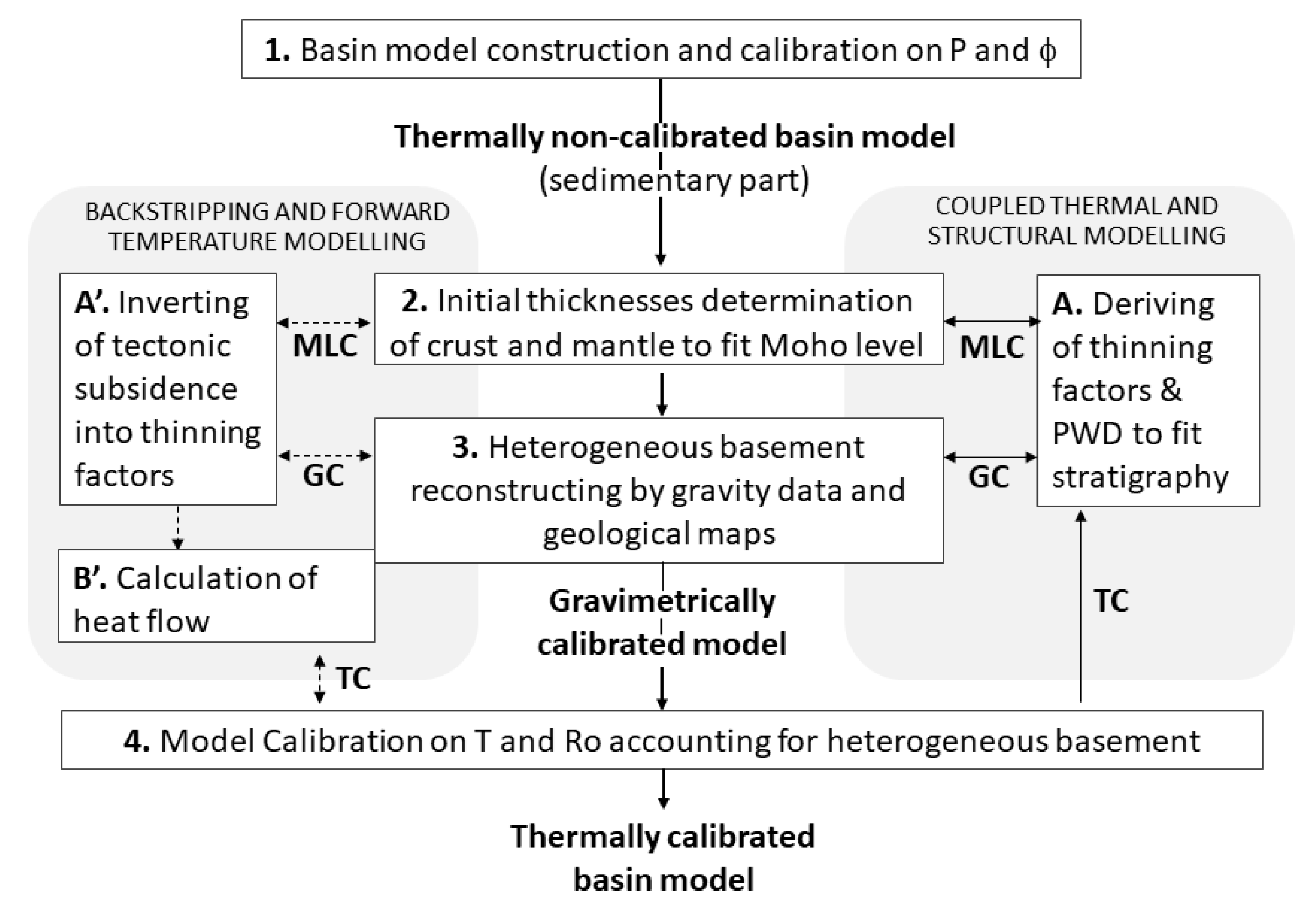
2. Method and Data

- The upper part of the basement is heterogeneous.
- Under the heterogeneous basement is a crystalline basement.
- The densities of the lithospheric layers, upper (ρu_crust) and lower (ρl_crust) crusts and the lithospheric mantle (ρl_mantle) are constant and change with temperature.
- The present-day width of each rectangular block is determined based on the basement maps.
- The first approximation of the thickness of each heterogeneous basement block is set.
- The physical properties of each heterogeneous block are based on the lithological descriptions of maps and their interpretations by standard mixing rules [21].
3. Central Part of the Western Siberian Basin
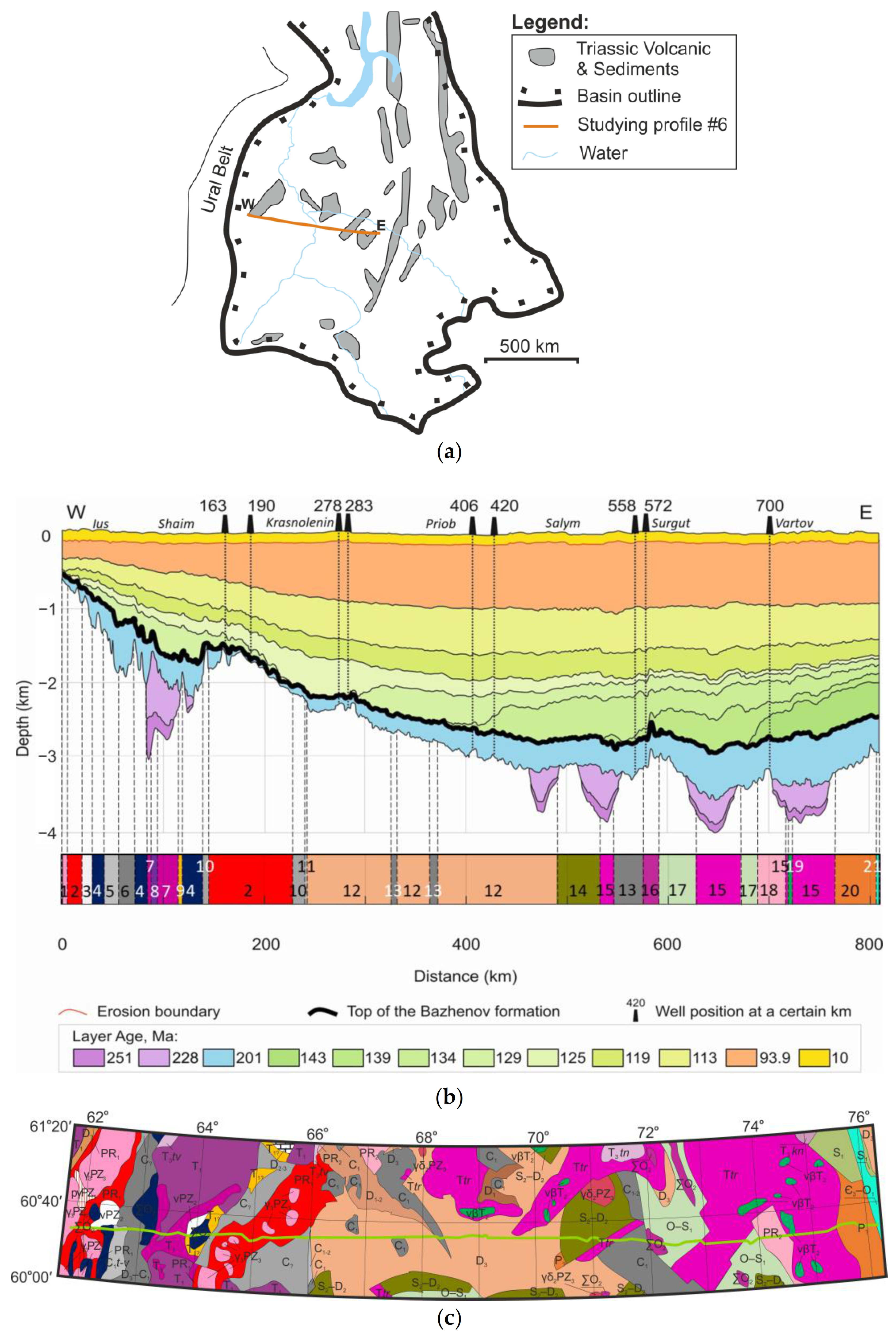
3.1. Geological Framework and Data Set
3.1.1. Heterogeneous Basement


| Unit No. | Colour | Lithology Description of Basement Units (Designation of Rocks by [44,45,46]) ◊ | Physical Properties A | |||||
|---|---|---|---|---|---|---|---|---|
| ρ | α | A | Сρ | λ | ||||
| (kg/m3) | (10−5 K−1) | (µW/m3) | (J/kg/K) | (W/m/K) | ||||
| 1 | Weathered granite; (γ3PZ3) | 2645 | (2500–2800) | 2.4 | 2 | 760 | 2.6 | |
| 2 | Sialitic gneiss, schist; (PR3) | 2600 | (2600 *–2620 *) | 2.4 | 2 | 850 | 3.0 | |
| 3 | Gabbro; (vPZ2) | 2870 | (2800–3100) | 1.6 | 0 | 800 | 2.9 | |
| 4 | Serpentinite, ultrabasit; (∑O2) | 3064 | (3100–3340) | 1.0 | 0 | 830 | 3.0 | |
| 5 | Terrigenous carbonate deposit; (C?) | 2766 | - | 2.6 | 1 | 890 | 2.4 | |
| 6 | Effusive rock; (D3–C1) | 2690 | - | 1.6 | 1 | 820 | 2.3 | |
| 7 | Effusive mixed tuff; (T1) | 2800 | (2780 *–3200) | 1.6 | 1 | 820 | 2.3 | |
| 8 | Basalt; (T1) | 2840 | (2780 *–3200) | 1.6 | 1 | 800 | 1.8 B | |
| 9 | Igneous–sedimentary rock; (T1?) | 2757 | - | 2.2 | 1 | 840 | 2.3 | |
| 10 | Terrigenous–schist rock; (C) | 2740 | - | 2.3 | 1 | 920 | 2.8 | |
| 11 | Organogenic limestone, sandstone, calcareous sandstone and siltstone, basalt, their tuff; (C1–2) | 2733 | - | 2.7 | 1 | 850 | 2.7 | |
| 12 | Clay and organogenic limestone, subordinate tufogenic–sedimentary rock, basalt; (D3) | 2767 | - | 2.7 | 1 | 840 | 2.8 | |
| 13 | Organogenic limestone, clay, carbonaceous schist, siltstone, marl, andesibasalt, rhyolite; (C1) | 2752 | - | 2.4 | 1 | 870 | 2.5 | |
| 14 | Siliceous and silty shale, siltstone, basalt, andesibasalt, their tuff, tufogenic–sedimentary rock, sandstone, gravelite; (S2–D2) | 2749 | - | 2.1 | 1 | 880 | 2.4 | |
| 15 | Basalt, dolerite, their tuff, tufogenic–sedimentary rock, mudstone, siltstone, sandstone, gravelite, andesite, rhyolite; (Ttr) | 2809 | (2750 *–3200) | 1.8 | 1 | 850 | 2.2 | |
| 16 | Serpentinized dunite, harzburgite, lerzolite, pyroxenite, serpentinite; (∑O2) | 2800 | (2750 *–2800 *) | 1.0 | 0 | 780 | 4.1 B | |
| 17 | Shale, siliceous shale, jasper, limestone, basalt, andesibasalt, their tuff; (O–S1) | 2712 | - | 2.5 | 1 | 860 | 2.7 | |
| 18 | Metamorphic schist, sericite–chlorite, sericite and carboneous phyllite, quartzite; (PR2) | 2840 | (2750 *–2900) | 2.7 | 1 | 900 | 2.8 | |
| 19 | Gabbrodolerite, dolerite; (vβT2) | 2909 | (2800–3100) | 1.7 | 0 | 860 | 2.4 | |
| 20 | Siltstone and tuff siltstone basalt, basalt clastolavas, andesite, tuffite, rhyolite; (P?) | 2721 | - | 2.1 | 1 | 860 | 2.0 | |
| 21 | Clay limestone, greenish-grey with lenses of organogenic clastic limestone; (Є3–O1) | 2728 | - | 2.4 | 1 | 850 | 2.3 | |
| Upper crust | 2700 | - | 2.4 | 2 | 1000 | 3.0 | ||
| Lower crust | 2900 | - | 2.4 | 2 | 1000 | 3.0 | ||
| Lithospheric mantle | 3340 | - | 3.2 | 0 | 1000 | 3.5 | ||
3.1.2. Rift Phases
3.1.3. Sedimentary Basin: Stratigraphy, Infill, Erosion
3.1.4. Petroleum Systems
3.1.5. Boundary Conditions
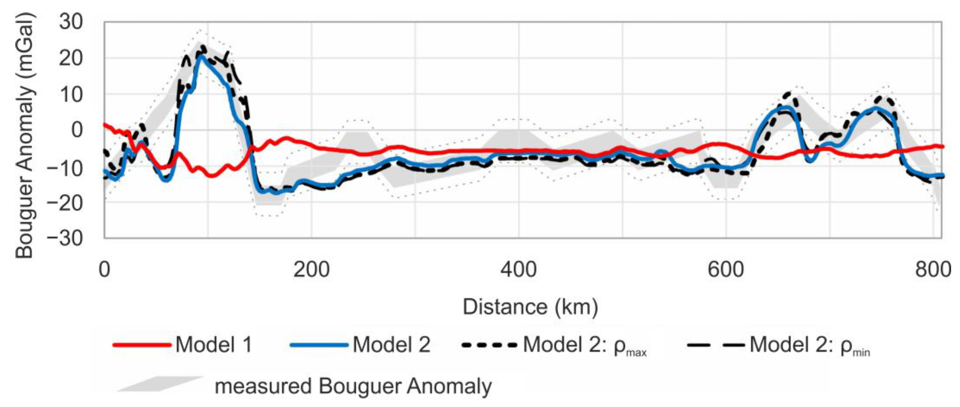
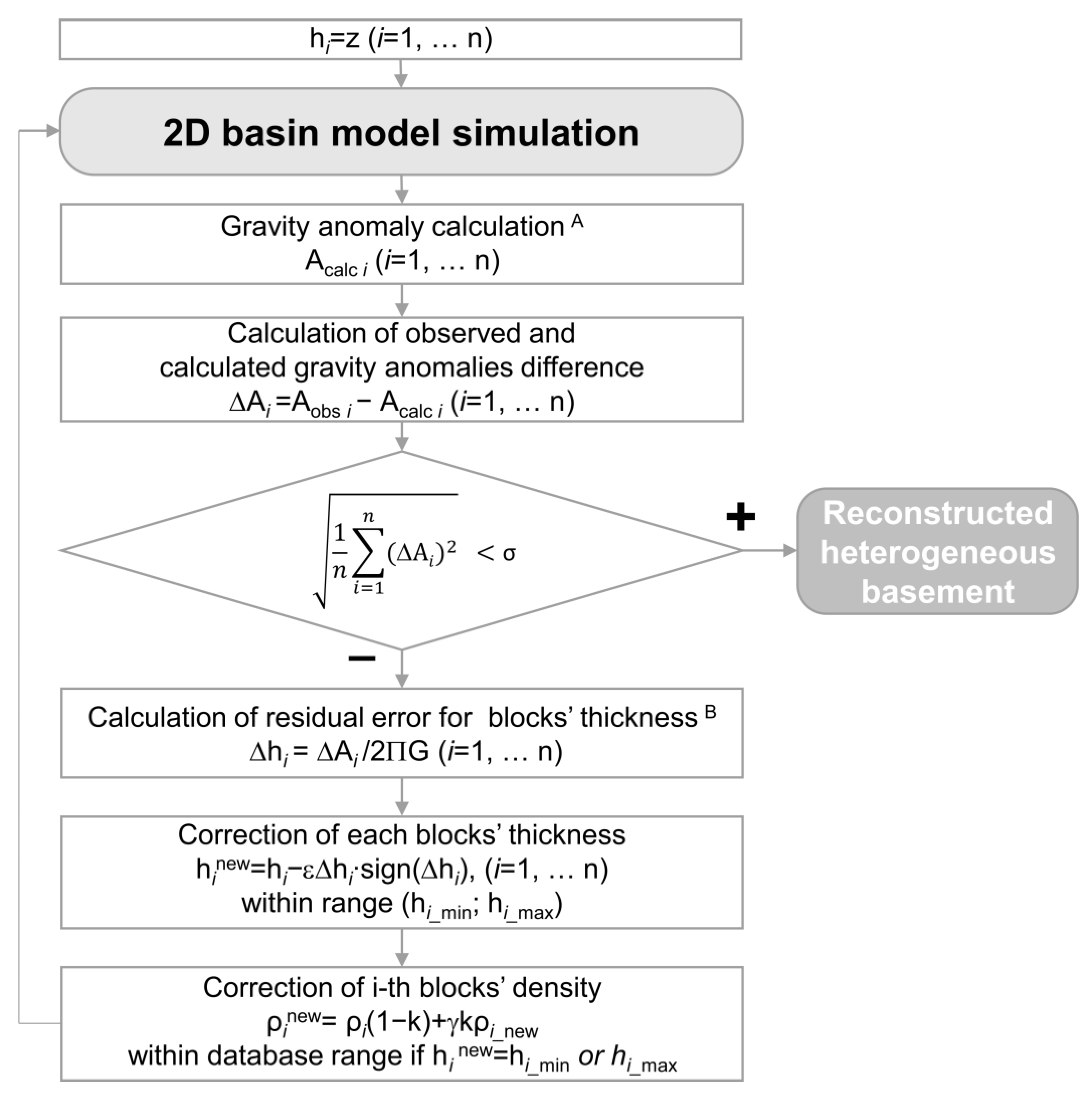
3.1.6. Gravity Anomaly Data
3.2. Construction and Calibration of Basin Models
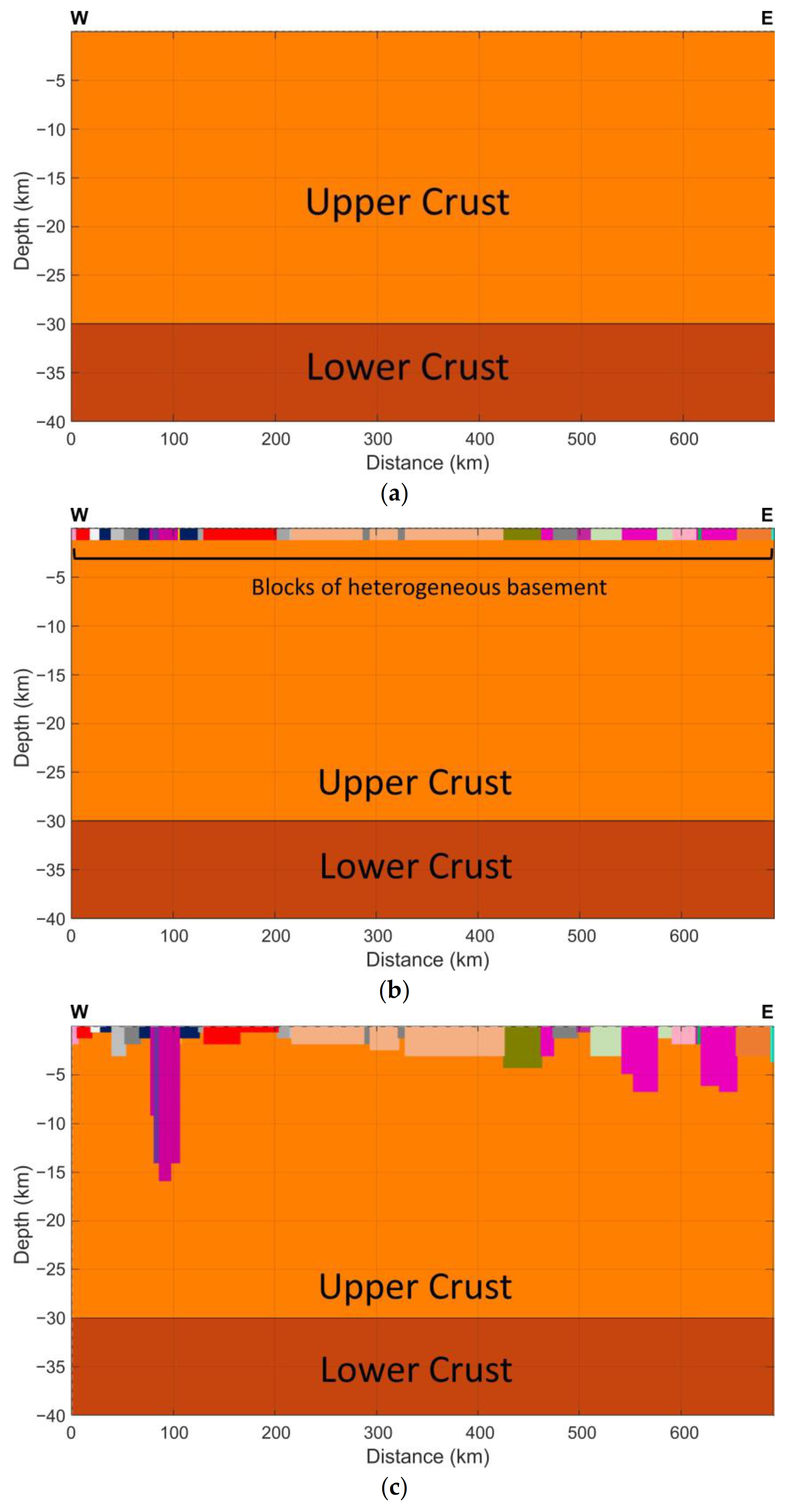
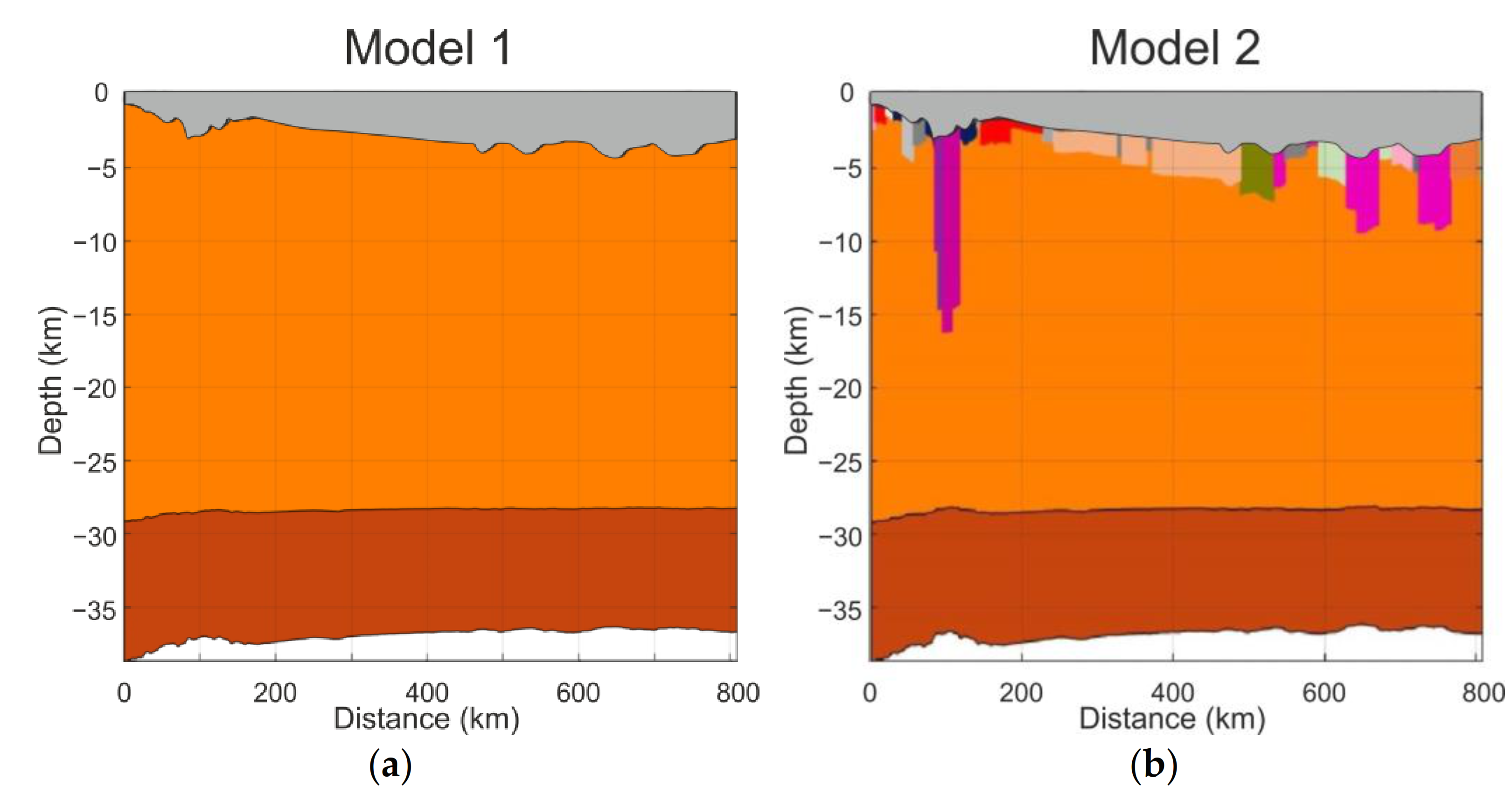
3.2.1. Construction of a Model with Homogeneous Basement: Model 1

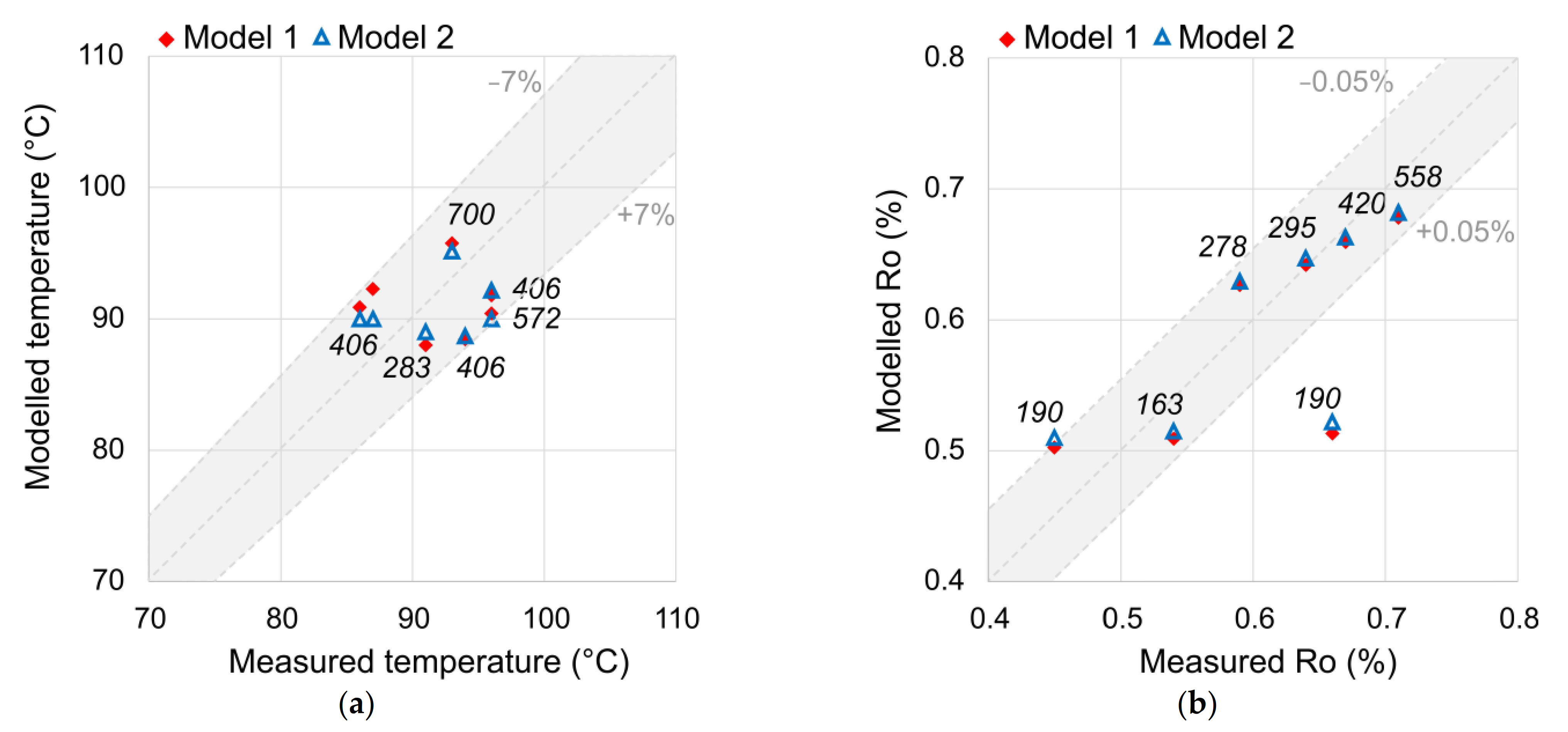
3.2.2. Calibration of Model 1
- A good match between the modelled stratigraphy and the input stratigraphy was obtained with an approximate convergence misfit of 5%. The result was reached after 15 inversion iterations of the forward modelling [7].
- The calculated present-day Moho depth is in good agreement with two published interpretations [37,42] within the interval of 190 km to the eastern end of the profile (Figure 3, red line). The absence of the flexural load by the Ural fold belt on the west in the model explains the discrepancy between the calculated and published data within the left interval of 0 to 190 km.
- The gravity anomaly (Figure 4, red line) was not fitted since the modelled σm = 10.5 mGal was greater than the desired accuracy of σ = 6.5 mGal.


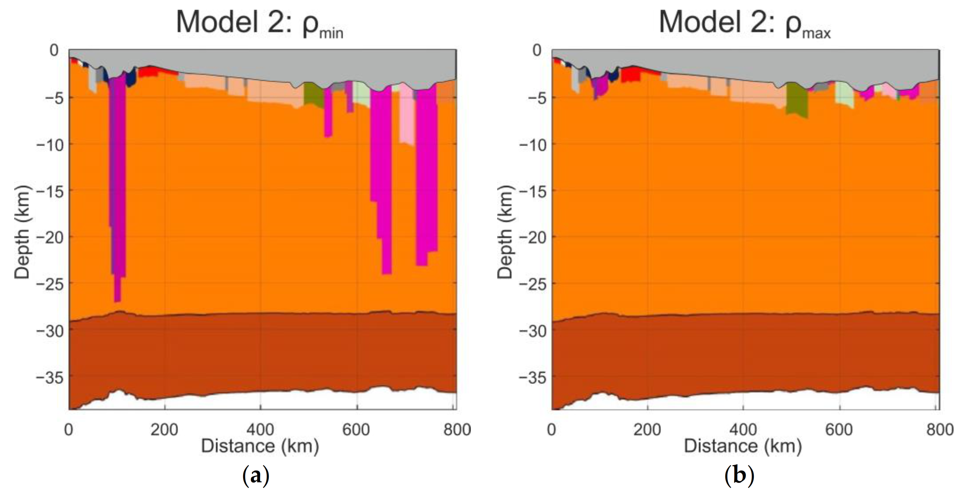
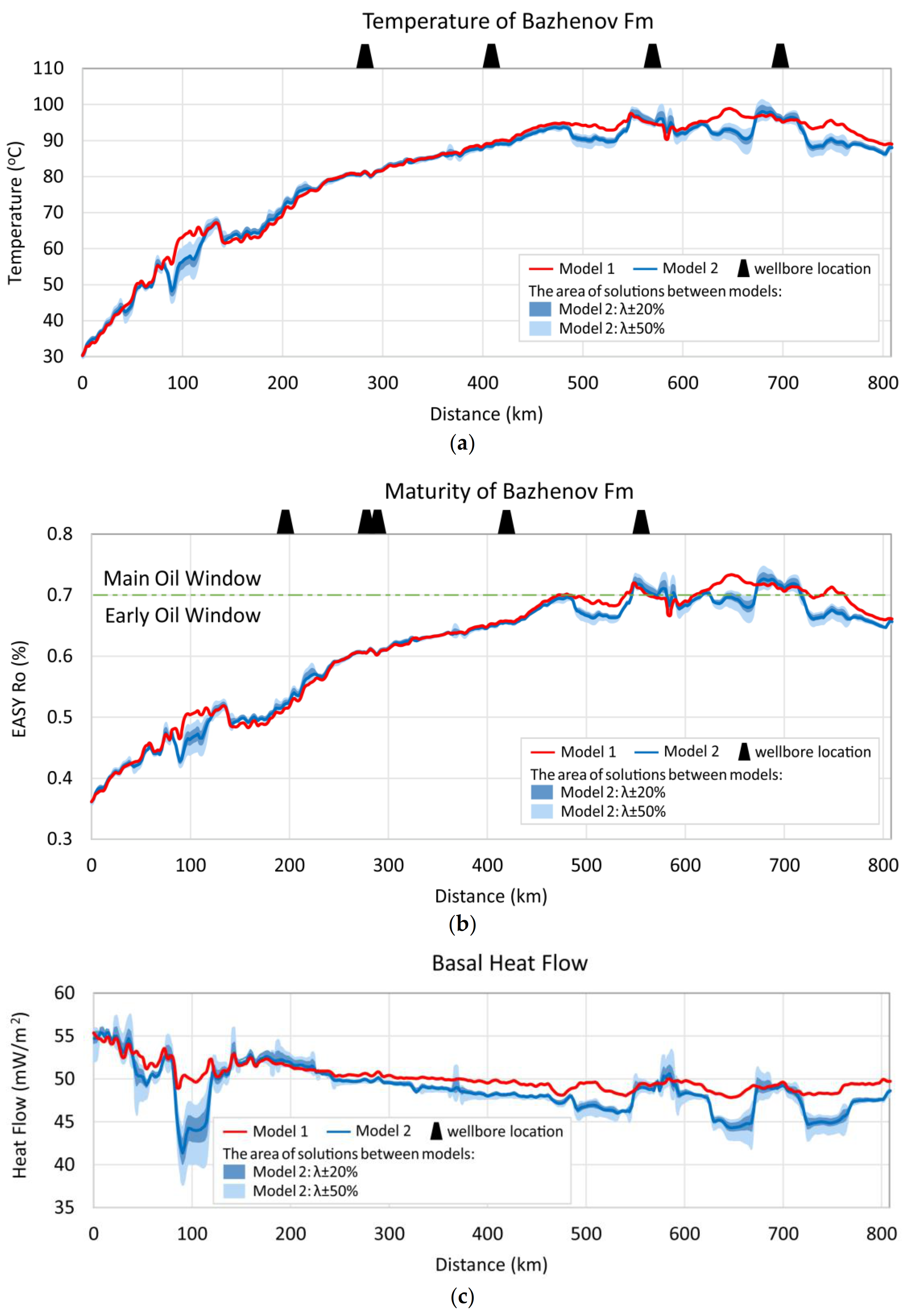
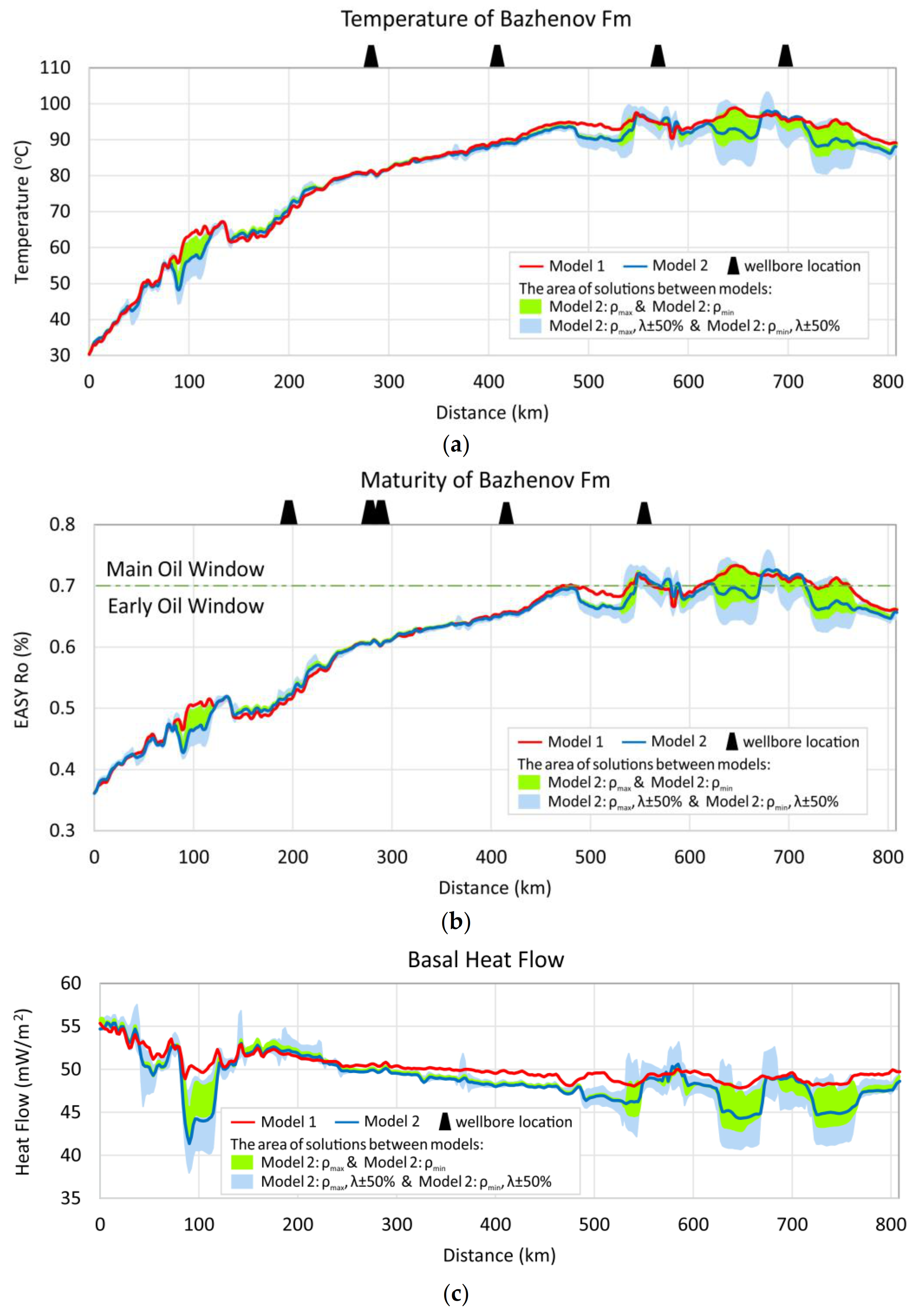
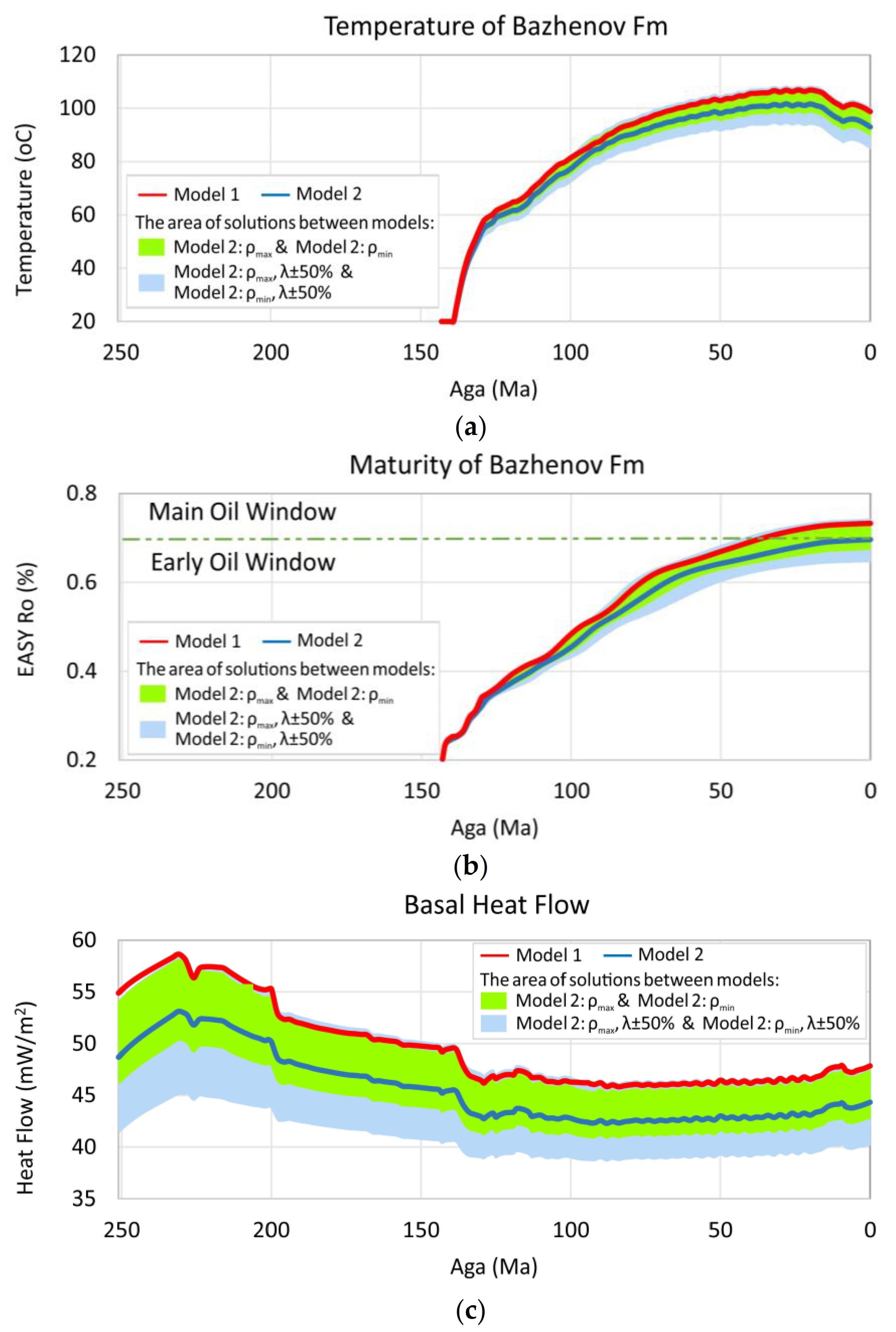
3.2.3. Construction of Models with the Heterogeneous Basement: Model 2, Model 2: ρmin and Model 2: ρmax
3.2.4. Calibration of Model 2, Model 2: ρmin and Model 2: ρmax
- The stratigraphy, porosity and pressure remained unchanged.
- The Moho depth stayed almost unchanged (Figure 3). A negligible difference with respect to Model 1 was observed only in rift-graben zones.
- The thermal regime was refined by the e-fold length parameter (Ar), which was slightly increased to 21 km (to compensate the decreased radiogenic heat production and thermal conductivity in the heterogeneous basement).
4. Results and Discussion
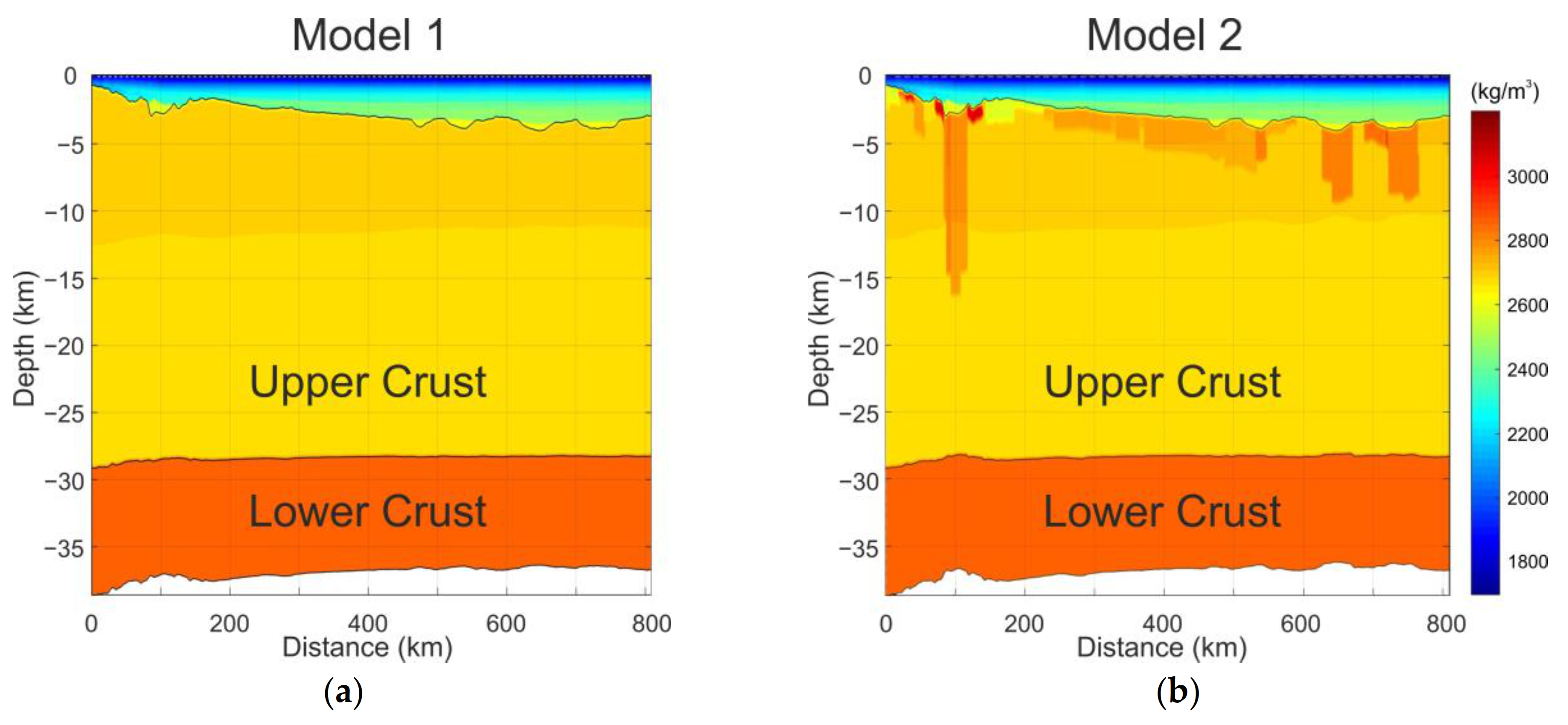
4.1. Results of Accounting for Heterogeneous Basement
4.1.1. Thicknesses of Basement Heterogeneity Blocks
4.1.2. Densities of the Basement
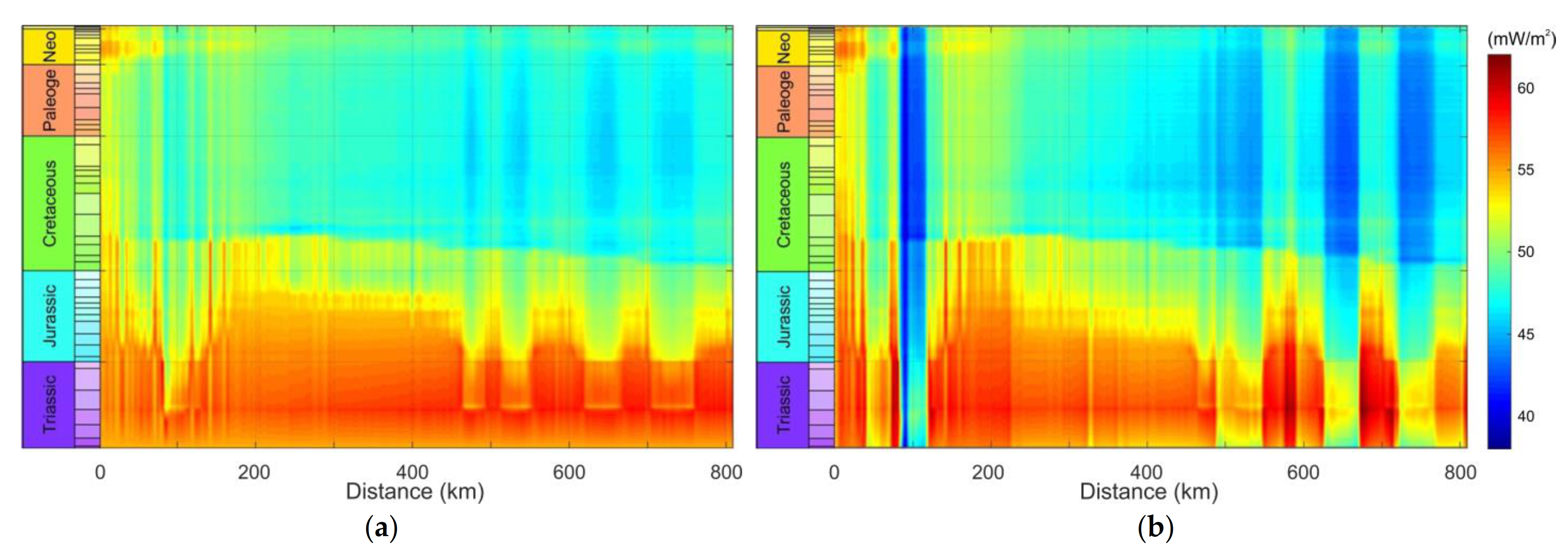
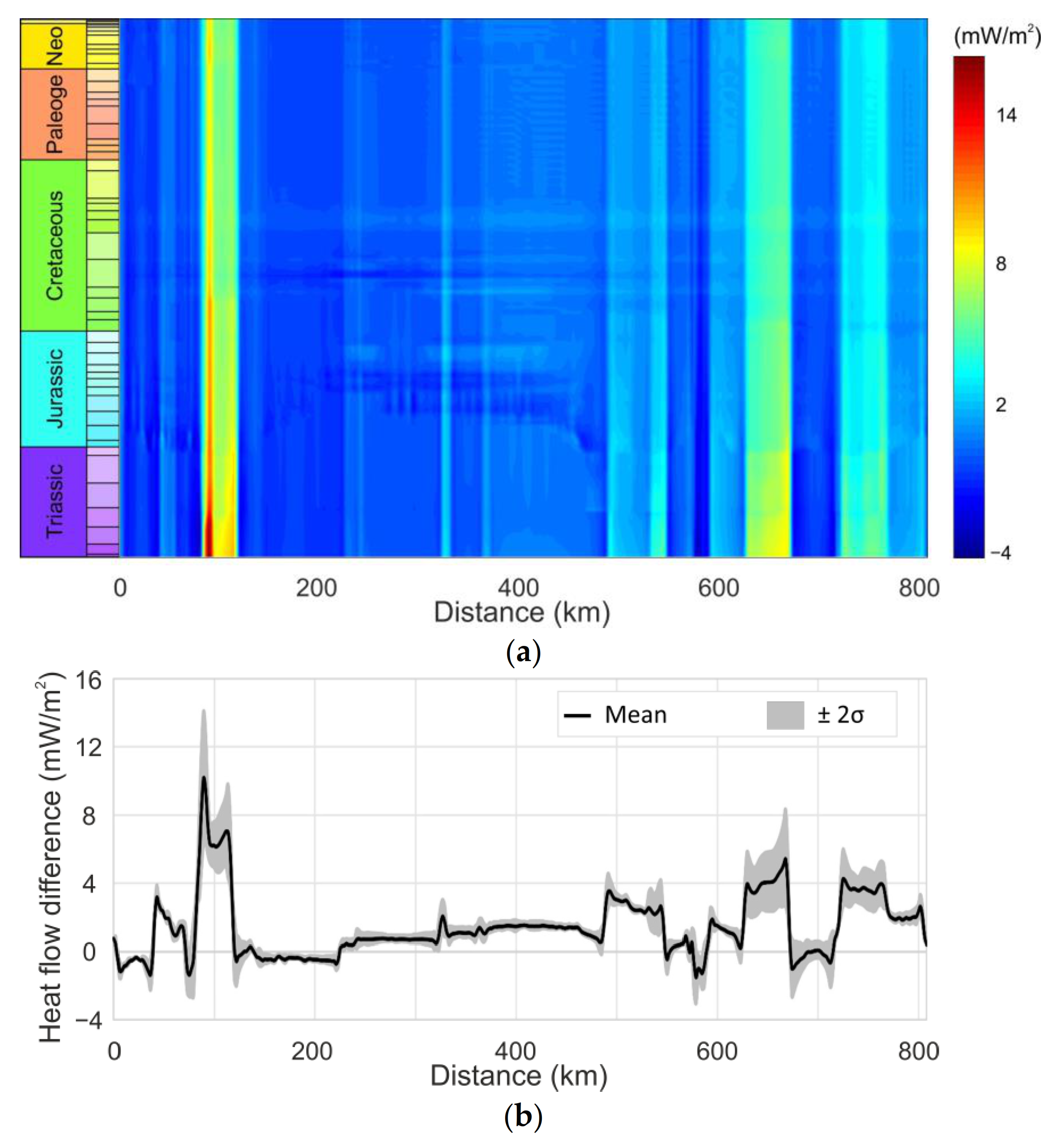
4.1.3. Thermal Regime


4.2. Analysis of Uncertainties in Characteristics of Heterogeneous Basement
4.2.1. Density Uncertainties


4.2.2. Thermal Conductivity Uncertainties
4.3. Summarising of the Express Estimation
5. Conclusions
Author Contributions
Funding
Data Availability Statement
Acknowledgments
Conflicts of Interest
Appendix A

Appendix B
| Age | Physical Properties * | |||||
|---|---|---|---|---|---|---|
| φ0 | B | ρ | λ | Сρ | A | |
| (Ma) | (1/km) | (kg/m3) | (W/m/K) | (J/kg/K) | (µW/m3) | |
| 0–93.9 | 0.63 | 0.69 | 2705 | 1.9 | 870 | 2 |
| 93.9–113 | 0.59 | 0.59 | 2711 | 2.85 | 880 | 1 |
| 113–119 | 0.49 | 0.41 | 2720 | 3.68 | 890 | 1 |
| 119–125 | 0.63 | 0.67 | 2706 | 2.82 | 870 | 2 |
| 125–129 | 0.52 | 0.48 | 2714 | 2.5 | 880 | 1 |
| 125–129 | 0.52 | 0.48 | 2714 | 3.7 | 870 | 1 |
| 129–134 | 0.52 | 0.48 | 2714 | 2.5 | 880 | 1 |
| 134–139 | 0.52 | 0.48 | 2714 | 2.5 | 880 | 1 |
| 139–143 | 0.52 | 0.48 | 2714 | 2.5 | 880 | 1 |
| 143–201 | 0.58 | 0.58 | 2629 | 2.65 | 860 | 2 |
| 201–251 | 0.15 | 0.23 | 2739 | 2.56 | 870 | 1 |
Appendix C
References
- Galushkin, Y.I. Sedimentary Basin Modeling and Estimation of Its Hydrocarbon Potential; Nauchnyi Mir: Moscow, Russia, 2007. [Google Scholar]
- Wangen, M. Physical Principles of Sedimentary Basin Analysis; Cambridge University Press: Cambridge, UK, 2010. [Google Scholar]
- Chekhonin, E.; Popov, Y.; Peshkov, G.; Spasennykh, M.; Popov, E.; Romushkevich, R. On the importance of rock thermal conductivity and heat flow density in basin and petroleum system modelling. Basin Res. 2019, 32, 1261–1276. [Google Scholar] [CrossRef]
- Clark, S.A.; Glorstad-Clark, E.; Faleide, J.I.; Schmid, D.; Hartz, E.H.; Fjeldskaar, W. Southwest Barents Sea rift basin evolution: Comparing results from backstripping and timeforward modelling. Basin Res. 2013, 26, 550–566. [Google Scholar] [CrossRef]
- Theissen, S.; Rüpke, L.H. Feedbacks of sedimentation on crustal heat flow: New insights from the Voring Basin, Norwegian Sea. Basin Res. 2010, 22, 976–990. [Google Scholar] [CrossRef]
- Peshkov, G.A.; Chekhonin, E.M.; Rüpke, L.H.; Musikhin, K.A.; Bogdanov, O.A.; Myasnikov, A.V. Impact of differing heat flow solutions on hydrocarbon generation predictions: A case study from West Siberian Basin. Mar. Pet. Geol. 2021, 124, 104807. [Google Scholar] [CrossRef]
- Rüpke, L.H.; Schmalholz, S.M.; Schmid, D.W.; Podladchikov, Y.Y. Automated thermotectonostratigraphic basin reconstruction: Viking Graben case study. AAPG Bull. 2008, 92, 309–326. [Google Scholar] [CrossRef]
- SEG Wiki online Dictionary. Available online: https://wiki.seg.org/wiki/Dictionary:Acoustic_basement (accessed on 10 November 2021).
- Oilfield Glossary, Schlumberger. Available online: https://glossary.oilfield.slb.com/en/terms/b/basement (accessed on 10 November 2021).
- Klitzke, P.; Sippel, J.; Faleide, J.I.; Scheck-Wenderoth, M. A 3D gravity and thermal model for the Barents Sea and Kara Sea. Tectonophysics 2016, 684, 131–147. [Google Scholar] [CrossRef]
- Klitzke, P.; Faleide, J.I.; Scheck-Wenderoth, M.; Sippel, J. A lithosphere-scale structural model of the Barents Sea and Kara Sea region. Solid Earth 2015, 6, 153–172. [Google Scholar] [CrossRef] [Green Version]
- Fjeldskaar, W.; Grunnaleite, I.; Zweigel, J.; Mjelde, R.; Faleide, J.I.; Wilson, J. Modelled palaeo-temperature on Vøring, offshore mid-Norway—The effect of the Lower Crustal Body. Tectonophysics 2009, 474, 544–558. [Google Scholar] [CrossRef]
- Scheck-Wenderoth, M.; Raum, T.; Faleide, J.I.; Mjelde, R.; Horsfield, B. The transition from the continent to the ocean: A deeper view on the Norwegian margin. J. Geol. Soc. 2007, 164, 855–868. [Google Scholar] [CrossRef]
- Scheck-Wenderoth, M.; Maystrenko, Y. How warm are passive continental margins? A 3-D lithosphere-scale study from the Norwegian margin. Geology 2008, 36, 419–422. [Google Scholar] [CrossRef]
- Fattah, R.A.; Meekes, J.A.C.; Colella, S.; Bouman, J.; Schmidt, M.; Ebbing, J. The application of GOCE satellite gravity data for basin and petroleum system modeling: A case-study from the Arabian Peninsula. Search Discov. Artic. 2013, 120130. [Google Scholar]
- Hansford, P.A. Basin Modelling of the South-West Barents Sea. Master’s Thesis, University of Oslo, Oslo, Norway, 2014. [Google Scholar]
- Robertson, E.C. Thermal Properties of Rocks; U.S. Geological Survey, Reston, VA, USA. 1988. [Google Scholar] [CrossRef] [Green Version]
- Haines, H.H. Thermal Expansion and Compressibility of Rocks as a Function of Pressure and Temperature. Master’s Thesis, Massachusetts Institute of Technology, Cambridge, MA, USA, 1982. [Google Scholar]
- Minakov, A.; Mjelde, R.; Faleide, J.I.; Flueh, E.R.; Dannowski, A.; Keers, H. Mafic intrusions east of Svalbard imaged by active-source seismic tomography. Tectonophysics 2012, 518–521, 106–118. [Google Scholar] [CrossRef]
- Peters, K.E.; Schenk, O.; Scheirer, A.H.; Wygrala, B.; Hantschel, T. Basin and Petroleum System Modeling. In Springer Handbook of Petroleum Technology; Springer: Berlin/Heidelberg, Germany, 2017; pp. 381–417. [Google Scholar]
- Hantschel, T.; Kauerauf, A.I. Fundamentals of Basin and Petroleum Systems Modeling; Springer Science & Business Media: Berlin/Heidelberg, Germany, 2009. [Google Scholar]
- Popov, E.Y.; Goncharov, A.; Popov, Y.A.; Spasennykh, M.; Chekhonin, E.; Shakirov, A.; Gabova, A. Advanced techniques for determining thermal properties on rock samples and cuttings and indirect estimating for atmospheric and formation conditions. IOP Conf. Ser. Earth Environ. Sci. 2019, 367, 12017. [Google Scholar] [CrossRef]
- Meshalkin, Y.; Shakirov, A.; Popov, E.; Koroteev, D.; Gurbatova, I. Robust well-log based determination of rock thermal conductivity through machine learning. Geophys. J. Int. 2020, 222, 978–988. [Google Scholar] [CrossRef]
- Bott, M.H.P. The use of rapid digital computing methods for direct gravity interpretation of sedimentary basins. Geophys. J. Int. 1960, 3, 63–67. [Google Scholar] [CrossRef] [Green Version]
- Heiland, C.A. Geophysical Exploration; Prentice Hall Inc.: Hoboken, NJ, USA, 1940. [Google Scholar]
- Waples, D.W. A New Model for Heat Flow in Extensional Basins: Radiogenic Heat, Asthenospheric Heat, and the McKenzie Model. Nat. Resour. Res. 2001, 10, 227–238. [Google Scholar] [CrossRef]
- Lachenbruch, A.H. Preliminary geothermal model of the Sierra Nevada. J. Geophys. Res. Space Phys. 1968, 73, 6977–6989. [Google Scholar] [CrossRef]
- Schön, J.H. Physical Properties of Rocks–A Workbook. In Handbook of Petroleum Exploration and Production; Elsevier: Oxford, UK, 2011. [Google Scholar]
- Hicks, P.J.J.; Fraticelli, C.M.; Shosa, J.D.; Hardy, M.J.; Townsley, M.B. Identifying and quantifying significant uncertainties in basin modeling. In Basin Modeling: New Horizons in Research and Applications; Peters, K.E., Curry, D.J., Kacewicz, M., Eds.; AAPG Hedberg Series; AAPG: Tulsa, OK, USA, 2012; Volume 4. [Google Scholar] [CrossRef]
- Ulmishek, G.F. Petroleum Geology and Resources of the West Siberian Basin, Russia; US Department of the Interior, US Geological Survey: Reston, VA, USA, 2003. [Google Scholar]
- Fjellanger, E.; Kontorovich, A.E.; Barboza, S.A.; Burshtein, L.M.; Hardy, M.J.; Livshits, V.R. Charging the giant gas fields of the NW Siberia basin. Geol. Soc. London Pet. Geol. Conf. Ser. 2010, 7, 659–668. [Google Scholar] [CrossRef]
- Kazanenkova, A. Some Aspects of Petroleum System Modeling in the North-Eastern Part of West Siberia Basin. Tyumen 2015-Deep Subsoil and Science Horizons. Eur. Assoc. Geosci. Eng. 2015, 2015, 1–5. [Google Scholar]
- Morozov, N.; Belenkaya, I.; Kasyanenko, A.; Bodryagin, S. Evaluation of the Resource Potential Based on 3D Basin Modeling of Bagenov Fm. Hydrocarbon System. In Proceedings of the SPE Russian Petroleum Technology Conference and Exhibition, Moscow, Russia, 24–26 October 2016; pp. 1–12. [Google Scholar] [CrossRef]
- Romanov, A.G.; Goncharov, I.V.; Gagarin, A.N.; Carruthers, D.J.; Corbett, P.W.M.; Ryazanov, A.V. 3D Modelling of the Hydrocarbon Migration in the Jurassic Petroleum System in Part of the West Siberia Basin. In Proceedings of the Canadian International Petroleum Conference, Calgary, Alberta, 7–9 June 2005; pp. 1–4. [Google Scholar] [CrossRef]
- Safronov, P.I.; Ershov, S.V.; Kim, N.S.; Fomin, A.N. Modeling of processes of generation, migration and accumulation of hydrocarbons in the Jurassic and Cretaceous complexes of the Yenisei-Khatanga Basin. Oil Gas Geol. 2011, 5, 48–55. [Google Scholar]
- Merkulov, V.P.; Volkova, A.A.; Grigoriev, G.S. The Using of 3D Modeling for Processing Gravimetric Data in the Study of Oil and Gas Deposits of the Pre-Jurassic Complex of Western Siberia. Geomodel 2019, 2019, 1–5. [Google Scholar] [CrossRef]
- Cherepanova, Y.; Artemieva, I.M.; Chemia, Z. Crustal structure of the Siberian craton and the West Siberian basin: An appraisal of existing seismic data. Tectonophysics 2013, 609, 154–183. [Google Scholar] [CrossRef] [Green Version]
- Stoupakova, A.; Sokolov, A.; Soboleva, E.; Kiryukhina, T.A.; Kurasov, I.A.; Bordyug, E. Geological survey and petroleum potential of Paleozoic deposits in the Western Siberia. Georesursy 2015, 61, 63–76. [Google Scholar] [CrossRef]
- Vyssotski, A.V.; Vyssotski, V.N.; Nezhdanov, A.A. Evolution of the West Siberian basin. Mar. Pet. Geol. 2006, 23, 93–126. [Google Scholar] [CrossRef]
- Kontorovich, A.E.; Surkov, V.S. Geology and Mineral Resources of Russia; VSEGEI: St. Petersburg, Russia, 2000; Volume 2. [Google Scholar]
- Kontorovich, A.E.; Nesterov, I.I.; Salmanov, F.K.; Surkov, V.S.; Trofimuk, A.A.; Ervye, Y.G. Geology of Oil and Gas of West Siberia; Nedra: Moscow, Russia, 1975. [Google Scholar]
- Braitenberg, C.; Ebbing, J. New insights into the basement structure of the West Siberian Basin from forward and inverse modeling of GRACE satellite gravity data. J. Geophys. Res. Earth Surf. 2009, 114. [Google Scholar] [CrossRef] [Green Version]
- Nikishin, A.M.; Ziegler, P.A.; Abbott, D.; Brunet, M.-F.; Cloetingh, S. Permo–Triassic intraplate magmatism and rifting in Eurasia: Implications for mantle plumes and mantle dynamics. Tectonophysics 2002, 351, 3–39. [Google Scholar] [CrossRef]
- Ivanov, K.S.; Koroteev, V.A.; Pecherkin, M.F.; Fedorov, Y.N.; Erokhin, Y.V. The western part of the West Siberian petroleum megabasin: Geologic history and structure of the basement. Russ. Geol. Geophys. 2009, 50, 365–379. [Google Scholar] [CrossRef]
- 45. Map of Jurassic Formations: P-42 (Khanty-Mansiysk). State Geological Map of the Russian Federation Third Generation West Siberian Series Map of Jurassic Formations Lying on the Foundation (Bottom View). Scale: 1: 1000000, Series: West Siberian, Compiled by: Geotex LLC, FSGBI “VSEGEI”, Editor: Kovrigina. 2009. Available online: http://www.geokniga.org/maps/7131 (accessed on 10 November 2021).
- 46. Map of Jurassic Formations: P-43 (Surgut). State Geological Map of the Russian Federation Third Generation Geological Map of Jurassic Formations Lying on the Foundation (Bottom View) West Siberian Series. Scale: 1: 1000000, Series: West Siberian, Compiled by: FSBI “VSEGEI”, FSUE ZapSibNIIIGG. 2010. Available online: http://www.geokniga.org/maps/7936 (accessed on 10 November 2021).
- Sekiguchi, K. A method for determining terrestrial heat flow in oil basinal areas. Tectonophysics 1984, 103, 67–79. [Google Scholar] [CrossRef]
- Allen, P.A.; Allen, J.R. Basin Analysis: Principles and Application to Petroleum Play Assessment, 3rd ed.; John Wiley & Sons: Hoboken, NJ, USA, 2013. [Google Scholar]
- Schön, J.H. Physical Properties of Rocks: Fundamentals and Principles of Petrophysics; Elsevier: Amsterdam, The Netherlands, 2015. [Google Scholar]
- Lee, E.Y.; Tejada, M.L.G.; Song, I.; Chun, S.S.; Gier, S.; Riquier, L.; White, L.T.; Schnetger, B.; Brumsack, H.; Jones, M.M.; et al. Petrophysical property modifications by alteration in a volcanic sequence at IODP Site U1513, Naturaliste Plateau. J. Geophys. Res. Solid Earth 2021, 126, e2020JB021061. [Google Scholar] [CrossRef]
- Clauser, C.; Huenges, E. Thermal conductivity of rocks and minerals. In Rock Physics and Phase Relations: A Handbook of Physical Constants; AGU: Washington, DC, USA, 1995; Volume 3, pp. 105–126. [Google Scholar]
- Kukkonen, I.T.; Jokinen, J.; Seipold, U. Temperature and pressure dependencies of thermal transport properties of rocks: Implications for uncertainties in thermal lithosphere models and new laboratory measurements of high-grade rocks in the central Fennoscandian shield. Surv. Geophys. 1999, 20, 33–59. [Google Scholar] [CrossRef]
- Norden, B.; Förster, A.; Förster, H.-J.; Fuchs, S. Temperature and pressure corrections applied to rock thermal conductivity: Impact on subsurface temperature prognosis and heat-flow determination in geothermal exploration. Geotherm. Energy 2020, 8, 1–19. [Google Scholar] [CrossRef]
- Duchkov, A.D.; Sokolova, L.S.; Ayunov, D.E. Database of Thermal Properties of Rocks of the Siberian Region of the Russian Federation. Certificate Number RU 2017621489. 25 October 2017. [Google Scholar]
- Seipold, U.; Schilling, F.R. Heat transport in serpentinites. Tectonophysics 2003, 370, 147–162. [Google Scholar] [CrossRef]
- Vibe, Y.; Bunge, H.-P.; Clark, S.R. Anomalous subsidence history of the West Siberian Basin as an indicator for episodes of mantle induced dynamic topography. Gondwana Res. 2018, 53, 99–109. [Google Scholar] [CrossRef]
- Surkov, V.S.; Smirnov, L.V. Tectonic Events of the Cenozoic and Phase Differentiation of Hydrocarbons in Hauterivian-Cenomanian Complex of West Siberian Basin. Geologiya Nefti Gaza. 1995, 11, 3–6. [Google Scholar]
- Deming, D.; Chapman, D.S. Thermal histories and hydrocarbon generation: Example from Utah-Wyoming thrust belt. AAPG Bull. 1989, 73, 1455–1471. [Google Scholar] [CrossRef]
- Woodside, W.; Messmer, J.H. Thermal conductivity of porous media. I. Unconsolidated sands. J. Appl. Phys. 1961, 32, 1688–1699. [Google Scholar] [CrossRef]
- Athy, L.F. Density, porosity, and compaction of sedimentary rocks. AAPG Bull. 1930, 14, 1–24. [Google Scholar] [CrossRef]
- Waples, D.W.; Waples, J.S. A review and evaluation of specific heat capacities of rocks, minerals, and subsurface fluids. Part 1: Minerals and nonporous rocks. Nat. Resour. Res. 2004, 13, 97–122. [Google Scholar] [CrossRef]
- Rudkevich, M.Y.; Ozeranskaya, L.S.; Chistyakova, N.F. Petroleum Complexes of Western Siberia Basin; Nedra: Moscow, Russia, 1988. [Google Scholar]
- Brekhuntsov, A.M.; Monastyrev, B.V.; Nesterov, I.I. Distribution patterns of oil and gas accumulations in West Siberia. Russ. Geol. Geophys. 2011, 52, 781–791. [Google Scholar] [CrossRef]
- Peters, K.E.; Kontorovich, A.E.; Huizinga, B.J.; Moldowan, J.M.; Lee, C.Y. Multiple Oil Families in the West Siberian Basin. AAPG Bull. 1994, 78, 893–909. [Google Scholar] [CrossRef]
- Ablya, E.; Nadezhkin, D.; Bordyug, E.; Korneva, T.; Kodlaeva, E.; Mukhutdinov, R.; Sugden, M.; Van Bergen, P. Paleozoic-sourced petroleum systems of the Western Siberian Basin–What is the evidence? Org. Geochem. 2008, 39, 1176–1184. [Google Scholar] [CrossRef]
- Isaev, V.I.; Rylova, T.B.; Gumerova, A.A. Paleoclimate of Western Siberia and Realization of the Generation Potential of Oil Source Deposits. Bull. Tomsk Polytech. Univ. 2014, 324, 93–101. [Google Scholar]
- Fischer, K.M.; Ford, H.A.; Abt, D.L.; Rychert, C.A. The lithosphere-asthenosphere boundary. Annu. Rev. Earth Planet. Sci. 2010, 38, 551–575. [Google Scholar] [CrossRef] [Green Version]
- Gravimetric Map of the Ural Federal District. Package of Operational Geological Information (GIS Atlas). VSEGEI. 2019. Available online: https://vsegei.ru/ru/info/gisatlas/ufo/okrug/f_22_gravika.jpg (accessed on 10 November 2021).
- Morelli, C.; Gantar, C.; McConnell, R.K.; Szabo, B.; Uotila, U. The International Gravity Standardization Net 1971 (IGSN 71); Osservatorio Geofisico Sperimentale: Trieste, Italy, 1972. [Google Scholar]
- Khmelevskoy, V.K.; Gorbachev, Y.I.; Kalinin, A.V.; Popov, M.G.; Seliverstov, N.I.; Shevnin, V.A. Geophysical research methods. In Textbook for Geological Specialties of Universities; KGPU: Petropavlovsk-Kamchatsky, Russia, 2004. [Google Scholar]
- Poplavskii, K.N.; Podladchikov, Y.Y.; Stephenson, R.A. Two-dimensional inverse modeling of sedimentary basin subsidence. J. Geophys. Res. Solid Earth 2001, 106, 6657–6671. [Google Scholar] [CrossRef] [Green Version]
- Čermák, V.; Rybach, L. Thermal conductivity and specific heat of minerals and rocks. In Landolt-Börnstein: Numerical Data and Functional Relationships in Science and Technology, New Series, Group V (Geophysics and Space Research), Volume Ia, (Physical Properties of Rocks); Angenheister, G., Ed.; Springer: Berlin/Heidelberg, Germany, 1982; pp. 305–343. [Google Scholar]
- Sweeney, J.J.; Burnham, A.K. Evaluation of a simple model of vitrinite reflectance based on chemical kinetics. AAPG Bull. 1990, 74, 1559–1570. [Google Scholar] [CrossRef]
- Nielsen, S.B.; Clausen, O.R.; McGregor, E. Basin%Ro: A vitrinite reflectance model derived from basin and laboratory data. Basin Res. 2017, 29, 515–536. [Google Scholar] [CrossRef]
- Schenk, O.; Peters, K.; Burnham, A. Evaluation of alternatives to Easy% Ro for calibration of basin and petroleum system models. In Proceedings of the 79th EAGE Conference and Exhibition, Paris, France, 12–15 June 2017; Volume 2017, pp. 1–5. [Google Scholar] [CrossRef]
- Nezhdanov, A.A.; Ogibenin, V.V.; Melnikova, M.V.; Smirnov, A.S. Structures and stratification of the Triassic-Jurassic formations in the northern part of Western Siberia. ROGTEC 2012, 31, 62–69. [Google Scholar]
- Blackbourn, G. The Palaeozoic of Western Siberia. ROGTEC 2014, 21, 12–23. [Google Scholar]
- Isaev, V.I.; Gulenok, R.Y.; Isaeva, O.S.; Lobova, G.A. Density modeling of the basement of sedimentary sequences and prediction of oil-gas accumulations: Evidence from South Sakhalin and West Siberia. Russ. J. Pac. Geol. 2008, 2, 191–204. [Google Scholar] [CrossRef]
- Kurchikov, A.R. Тhe geothermal regime of hydrocarbon pools in West Siberia. Geol. Geophys. 2001, 42, 1846–1853. [Google Scholar]
- Tissot, B.P.; Welte, D.H. Petroleum Formation and Occurrence, 2nd ed.; Springer: Berlin/Heidelberg, Germany, 1984. [Google Scholar]
- Wangen, M. The blanketing effect in sedimentary basins. Basin Res. 1995, 7, 283–298. [Google Scholar] [CrossRef]
- Lucazeau, F.; Le Douaran, S. The blanketing effect of sediments in basins formed by extension: A numerical model. Application to the Gulf of Lion and Viking graben. Earth Planet. Sci. Lett. 1985, 74, 92–102. [Google Scholar] [CrossRef]
- Kim, Y.; Huh, M.; Lee, E.Y. Numerical Modelling to Evaluate Sedimentation Effects on Heat Flow and Subsidence during Continental Rifting. Geosciences 2020, 10, 451. [Google Scholar] [CrossRef]
- Essa, K.S. A fast interpretation method for inverse modeling of residual gravity anomalies caused by simple geometry. J. Geol. Res. 2012, 2012, 327037. [Google Scholar] [CrossRef] [Green Version]
- Martyshko, P.S.; Ladovskii, I.V.; Byzov, D.D.; Tsidaev, A.G. Gravity data inversion with method of local corrections for finite elements models. Geosciences 2018, 8, 373. [Google Scholar] [CrossRef] [Green Version]
- Christensen, N.I.; Mooney, W.D. Seismic velocity structure and composition of the continental crust: A global view. J. Geophys. Res. Solid Earth 1995, 100, 9761–9788. [Google Scholar] [CrossRef]
- Kurchikov, A.R.; Stavitsky, B. Geothermy of Oil and Gas Bearing Areas of Western Siberia; Nedra: Moscow, Russia, 1987. [Google Scholar]
- National Standard of the Russian Federation Р 55659-2013. (ISO 7404-5:2009); Methods for the Petrographic Analysis of Coals. Part 5: Method of Determining the Reflectance of Vitrinite 2015; Standartinform: Moscow, Russia, 2015.
- ASTM D2798-20; Standard Test Method for Microscopical Determination of the Vitrinite Reflectance of Coal. ASTM International: West Conshohocken, PA, USA, 2020. [CrossRef]
- International Committee for Coal Petrology (ICCP). International Handbook of Coal Petrography (Supplement to 2nd ed.); CNRS, Academy of Sciences of the USSR: Paris, France, 1971. [Google Scholar]
- Komorek, J.; Morga, R. Relationship between the maximum and the random reflectance of vitrinite for coal from the Upper Silesian Coal Basin (Poland). Fuel 2002, 81, 969–971. [Google Scholar] [CrossRef]
- Hackley, P.; Araujo, C.V.; Borrego, A.; Bouzinos, A.; Cardott, B.J.; Cook, A.C.; Eble, C.; Flores, D.; Gentzis, T.; Gonçalves, P.A.; et al. Standardization of reflectance measurements in dispersed organic matter: Results of an exercise to improve interlaboratory agreement. Mar. Pet. Geol. 2015, 59, 22–34. [Google Scholar] [CrossRef]
- ASTM D7708-14; Standard Test Method for Microscopical Determination of the Reflectance of Vitrinite Dispersed in Sedimentary Rocks; ASTM International: West Conshohocken, PA, USA, 2014.
- Houseknecht, D.; Matthews, S. Thermal maturity of Carboniferous strata, Ouachita Mountains. AAPG Bull. 1985, 69, 335–345. [Google Scholar] [CrossRef]
- Vtorushina, E.A.; Bulatov, T.D.; Kozlov, I.V.; Vtorushin, M.N. The advanced technique for determination of pyrolysis parameters of rocks. Oil Gas Geol. 2018, 2, 71–77. [Google Scholar] [CrossRef]
- Yang, S.; Horsfield, B. Critical review of the uncertainty of Tmax in revealing the thermal maturity of organic matter in sedimentary rocks. Int. J. Coal Geol. 2020, 225, 103500. [Google Scholar] [CrossRef]
- Wust, R.A.J.; Nassichuk, B.R.; Brezovski, R.; Hackley, P.C.; Willment, N. Vitrinite reflectance versus pyrolysis Tmax data: Assessing thermal maturity in shale plays with special reference to the Duvernay shale play of the Western Canadian Sedimentary Basin, Alberta, Canada. In Proceedings of the SPE Unconventional Resources Conference and Exhibition-Asia Pacific, Society of Petroleum Engineers, Brisbane, Australia, 11–13 November 2013. [Google Scholar] [CrossRef] [Green Version]
- Jarvie, D.M.; Claxton, B.L.; Henk, F.; Breyer, J.T. Oil and shale gas from the Barnett Shale, Ft. Worth Basin, Texas. AAPG Annu. Meet. Program 2001, 10, A100. [Google Scholar]
- Blackwell, D.D.; Spafford, R.E. 14. Experimental Methods in Continental Heat Flow. Methods Exp. Phys. 1987, 24, 189–226. [Google Scholar]
- Hermanrud, C.; Cao, S.; Lerche, I. Estimates of virgin rock temperature derived from BHT measurements: Bias and error. Geophysics 1990, 55, 924–931. [Google Scholar] [CrossRef]
- Waples, D.W.; Ramly, M. A statistical method for correcting log-derived temperatures. Pet. Geosci. 2001, 7, 231–240. [Google Scholar] [CrossRef]
- Förster, A. Analysis of borehole temperature data in the Northeast German Basin: Continuous logs versus bottom-hole temperatures. Pet. Geosci. 2001, 7, 241–254. [Google Scholar] [CrossRef] [Green Version]
- Gallardo, J.; Blackwell, D.D. Thermal structure of the Anadarko Basin. AAPG Bull. 1999, 83, 333–361. [Google Scholar] [CrossRef]
- Schumacher, S.; Moeck, I. A new method for correcting temperature log profiles in low-enthalpy plays. Geotherm. Energy 2020, 8, 27. [Google Scholar] [CrossRef]
- Peters, K.E.; Nelson, P.H. Criteria to determine borehole formation temperatures for calibration of basin and petroleum system models. SEPM Spec. Publ. 2012, 103, 5–15. [Google Scholar]
- LaFehr, T.R. Standardization in gravity reduction. Geophysics 1991, 56, 1170–1178. [Google Scholar] [CrossRef]
- Chapin, D.A. The theory of the Bouguer gravity anomaly: A tutorial. Lead. Edge 1996, 15, 361–363. [Google Scholar] [CrossRef]
- Jacoby, W.; Smilde, P.L. Gravity Interpretation: Fundamentals and Application of Gravity Inversion and Geological Interpretation; Springer Science & Business Media: Berlin/Heidelberg, Germany, 2009. [Google Scholar]
- Talwani, M. Errors in the total Bouguer reduction. Geophysics 1998, 63, 1125–1130. [Google Scholar] [CrossRef]


Publisher’s Note: MDPI stays neutral with regard to jurisdictional claims in published maps and institutional affiliations. |
© 2022 by the authors. Licensee MDPI, Basel, Switzerland. This article is an open access article distributed under the terms and conditions of the Creative Commons Attribution (CC BY) license (https://creativecommons.org/licenses/by/4.0/).
Share and Cite
Peshkov, G.A.; Chekhonin, E.M.; Pissarenko, D.V. Estimation of the Impact of Basement Heterogeneity on Thermal History Reconstruction: The Western Siberian Basin. Minerals 2022, 12, 97. https://doi.org/10.3390/min12010097
Peshkov GA, Chekhonin EM, Pissarenko DV. Estimation of the Impact of Basement Heterogeneity on Thermal History Reconstruction: The Western Siberian Basin. Minerals. 2022; 12(1):97. https://doi.org/10.3390/min12010097
Chicago/Turabian StylePeshkov, Georgy Alexandrovich, Evgeny Mikhailovich Chekhonin, and Dimitri Vladilenovich Pissarenko. 2022. "Estimation of the Impact of Basement Heterogeneity on Thermal History Reconstruction: The Western Siberian Basin" Minerals 12, no. 1: 97. https://doi.org/10.3390/min12010097