
Elemental Enrichment in Shallow Subsurface Red Sea Coastal Sediments, Al-Shuaiba, Saudi Arabia: Natural vs. Anthropogenic Controls


Abstract
:1. Introduction
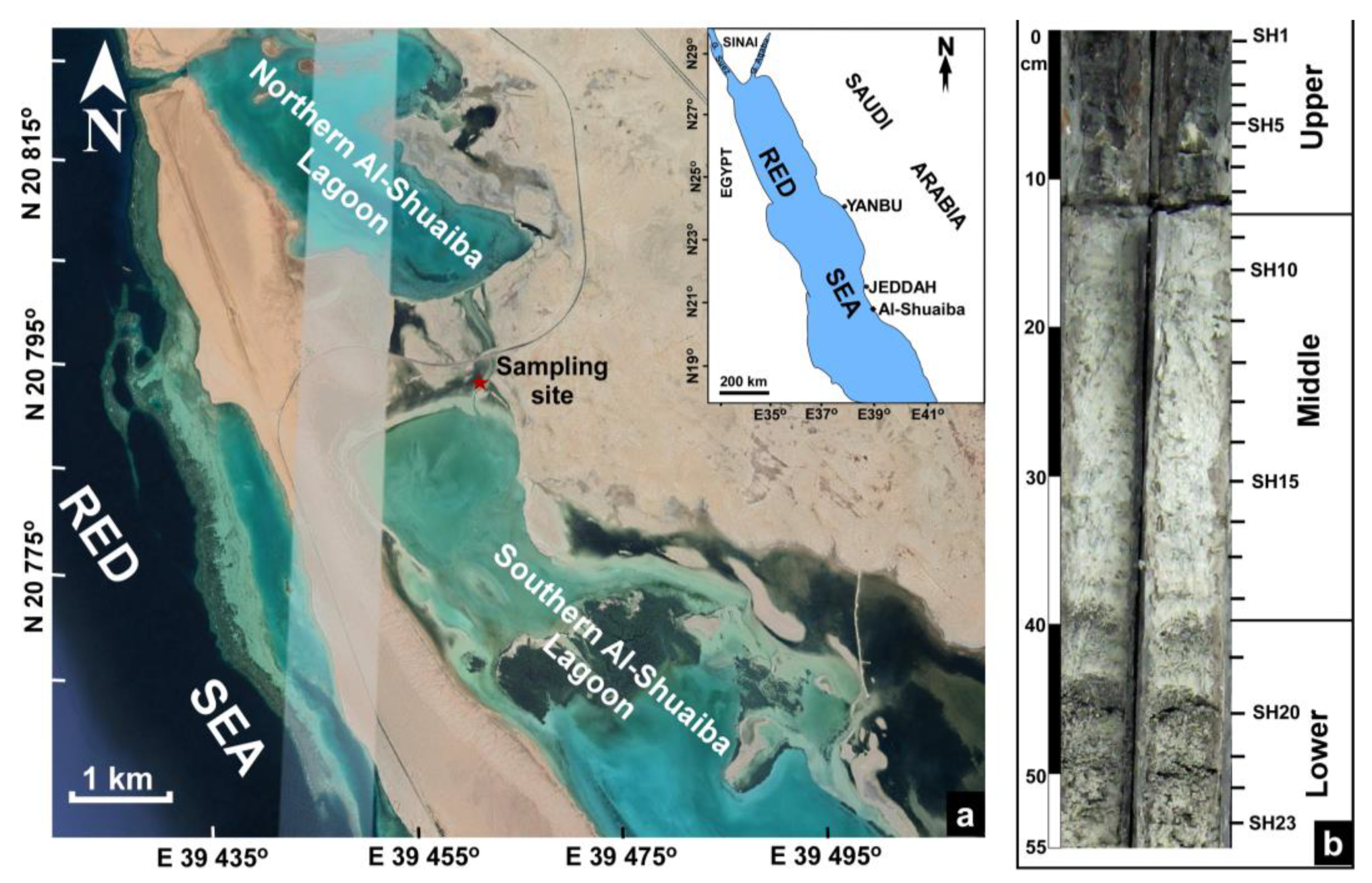
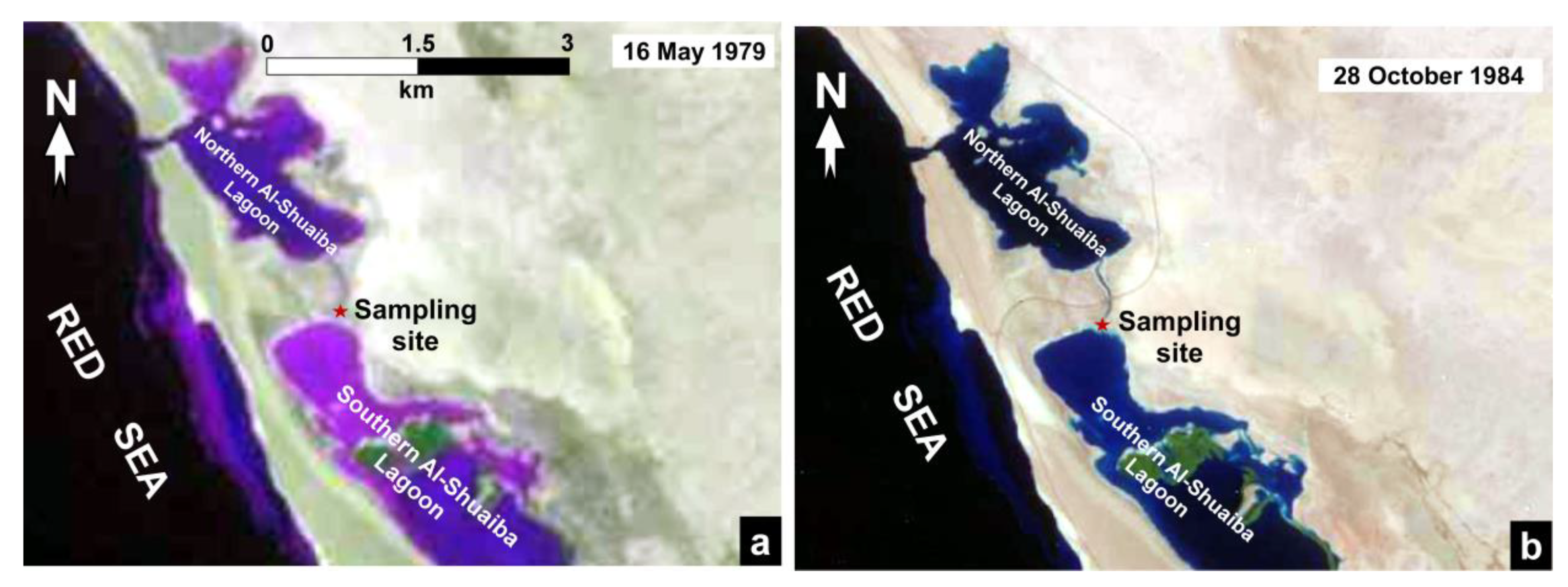
2. Area of Study
3. Materials and Methods
4. Results
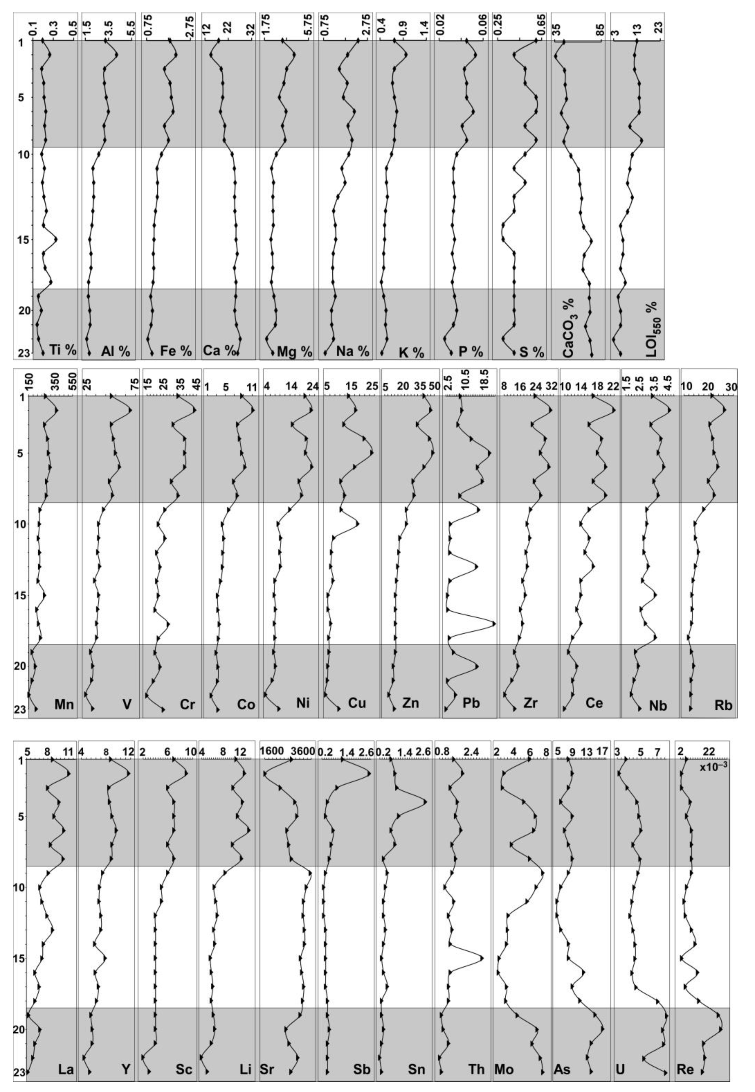
4.1. Chemical Composition
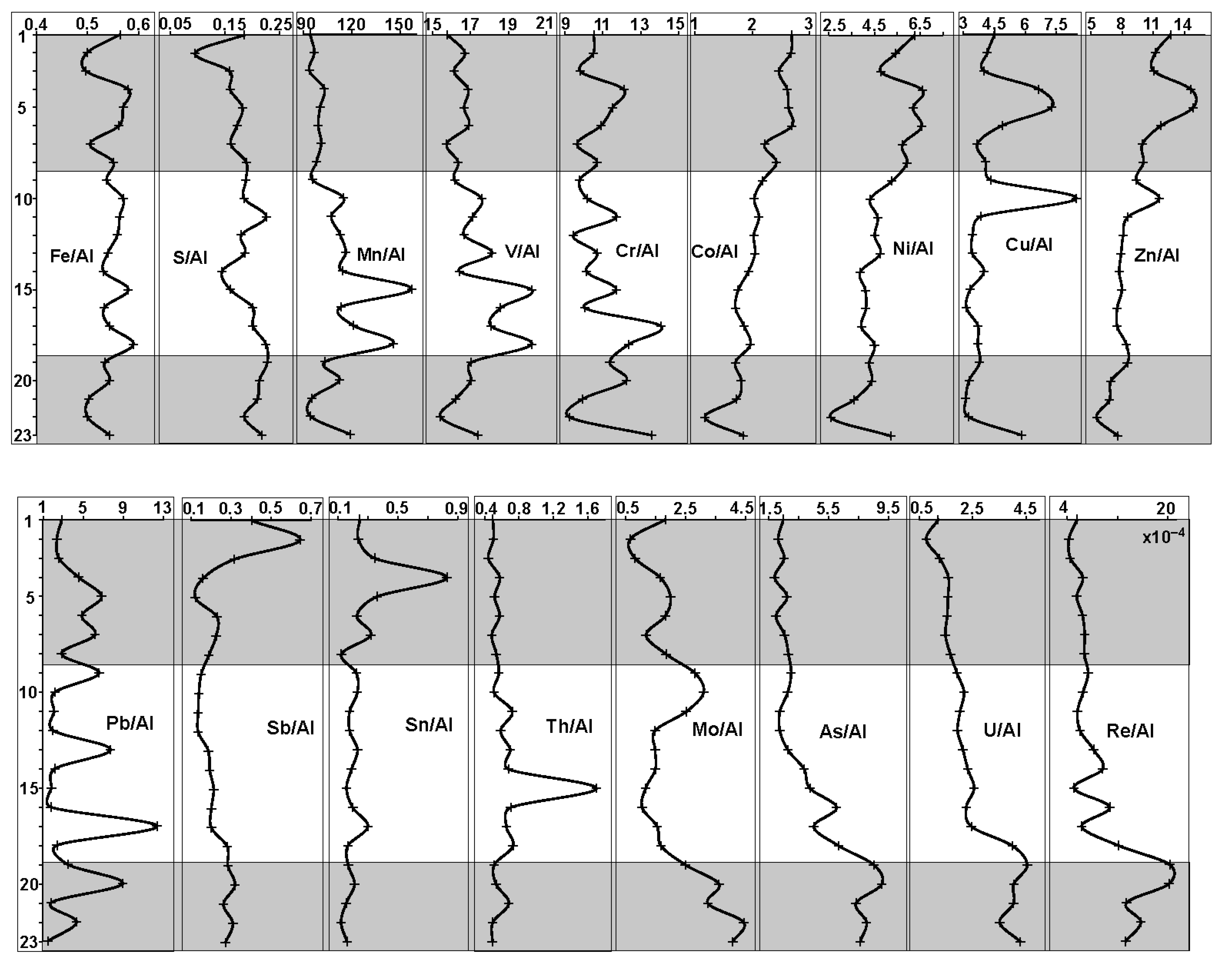
4.2. Enrichment Factor
4.3. Statistical Analysis
5. Discussion
Redox-Sensitive Elements
6. Conclusions
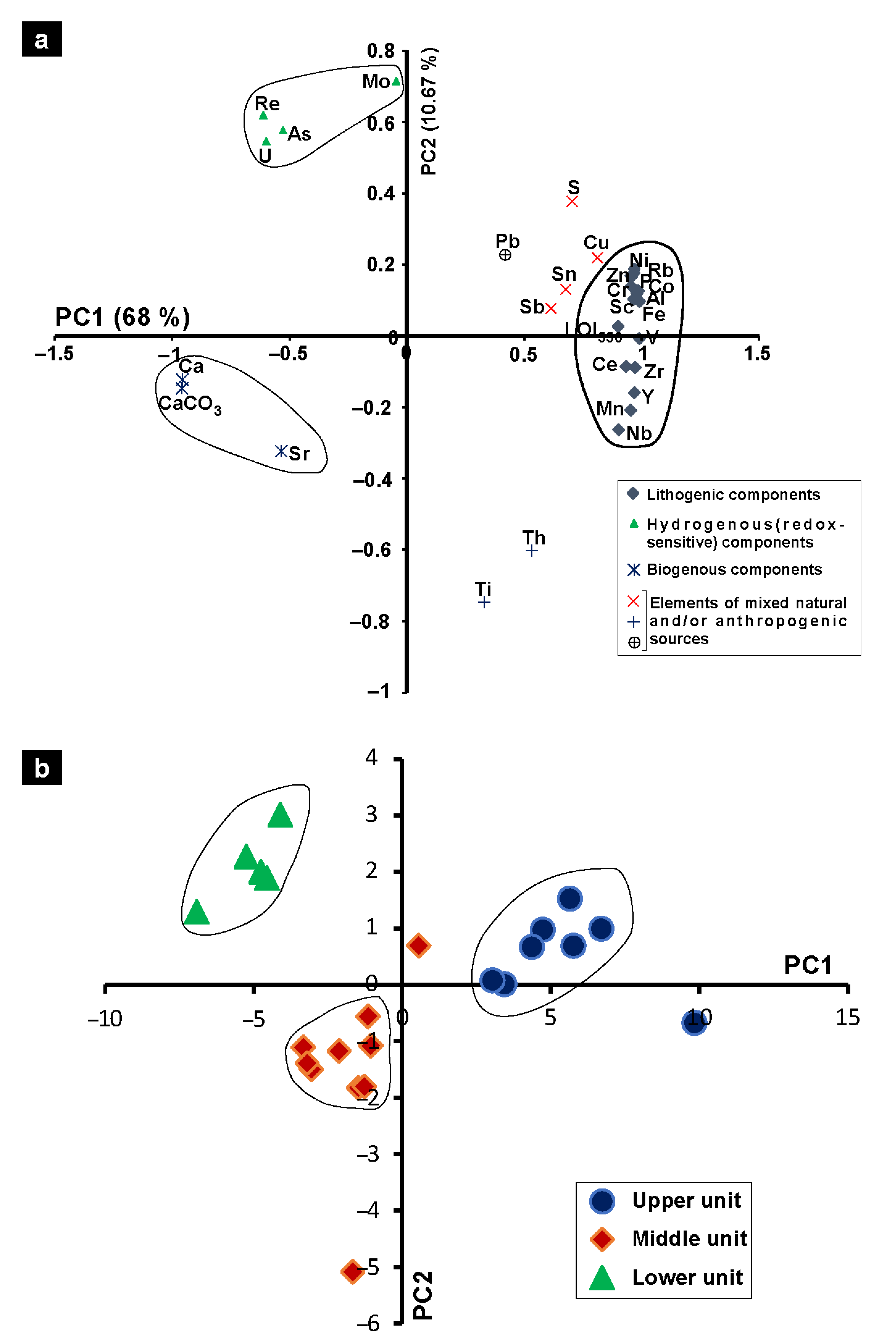
- Based on the colour of sediments, vertical variation in elemental concentrations, and statistical analysis, the core was subdivided into three units, upper, middle, and lower.
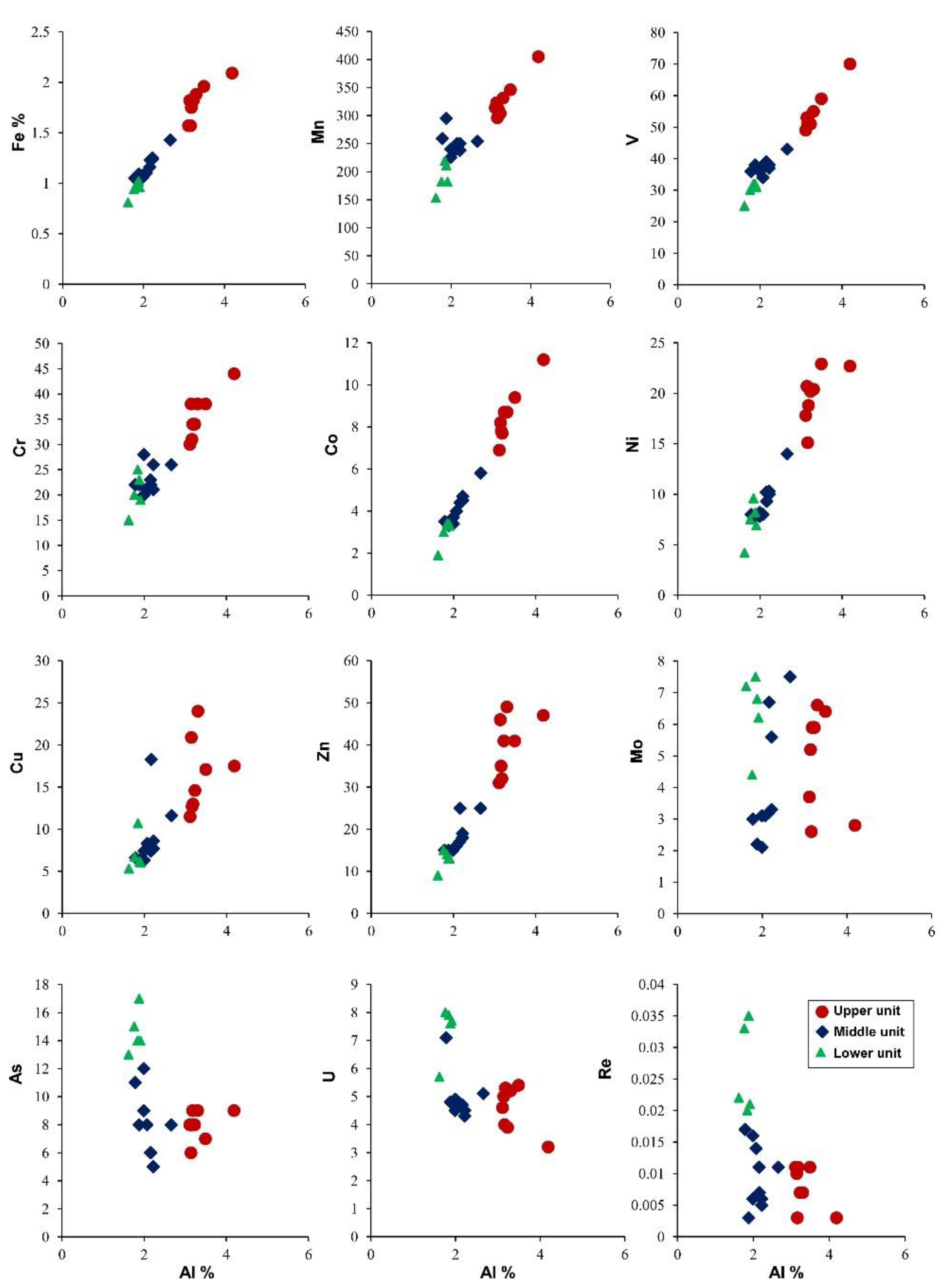
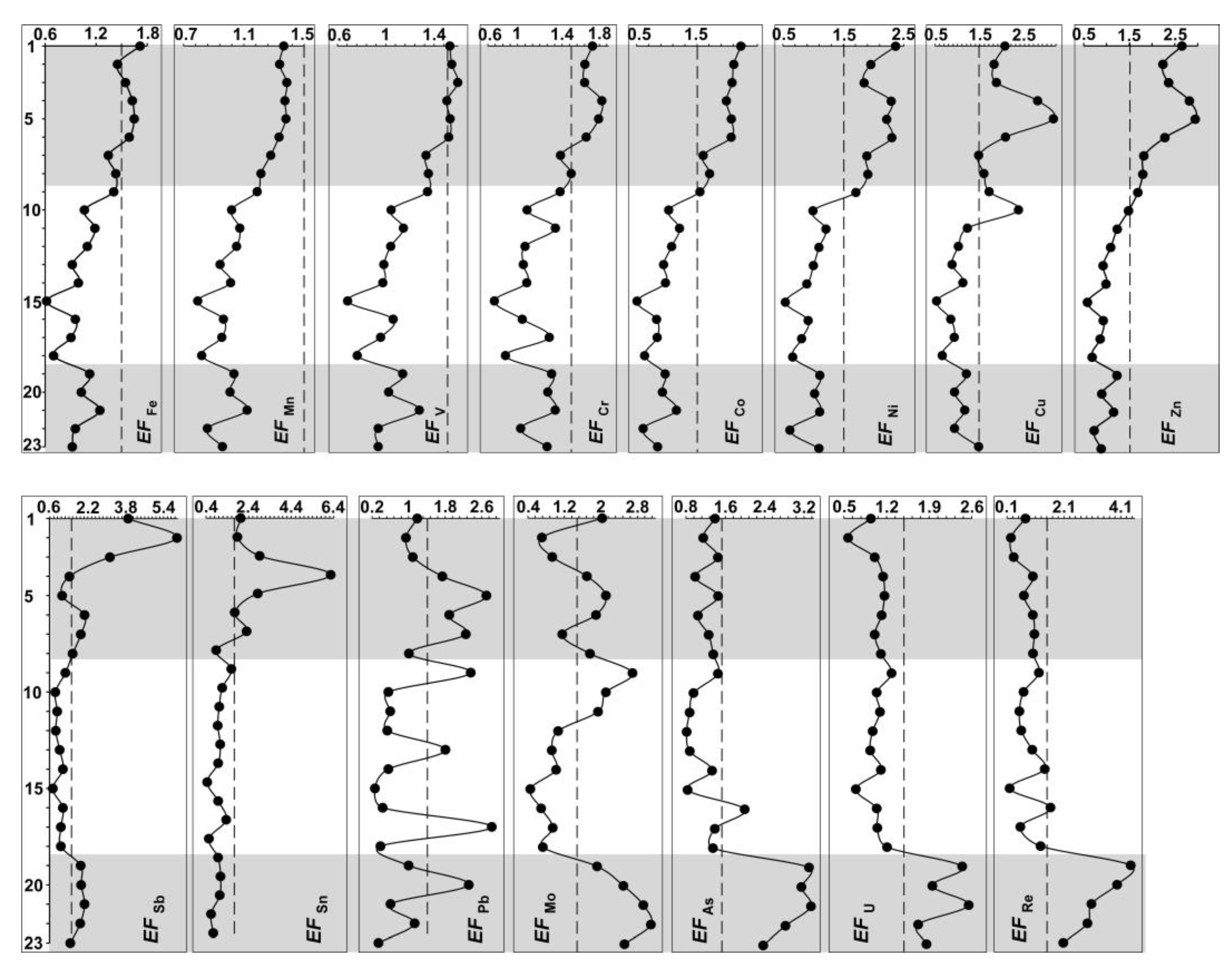
- The upper organic-rich unit shows enrichment of lithogenous elements and values of LOI550 (organic matter) content. Trace elements Mn, V, Cr, Co, Ni, and Zn display significant positive correlations with Al suggesting their lithogenic source. Though these elements are derived from a lithogenic source, their enrichment is related to human activity. This level is attributed to the road construction between the two lagoons. The relatively high concentrations of Pb and Cu in the upper unit are possibly related to atmospheric road dust and from the increasing movement of cars. Though the road construction limited the water circulation between the two lagoons, the sediments were deposited under oxic conditions as shown by the depletion of redox-sensitive elements.
- The lower and middle units of the core contain relatively higher carbonate content than the upper part. Strontium (Sr) distribution appears to be controlled by the presence of biogenic carbonate minerals. Calcium (Ca) distribution follows largely the spatial distribution of the carbonate content since Ca, Sr, and CaCO3 are biogenic components.
- The chemical composition of the lower unit suggests deposition in poorly circulated bottom water, with prevailing suboxic or even anoxic conditions probably related to the solar forcing (Medieval climate anomaly). This is confirmed by depletions in Mn and Co and relative enrichment of Mo, As, U, and Re. The distribution pattern of the Al-normalized redox sensitive elements is characterized by markedly high values in the lower unit. They display a negative to poor correlation with Al excluding lithogenic sources. Molybdenum (Mo), As, U, and Re are reliable and most promise proxies for redox conditions since they behave conservatively in oxygenated waters and are enriched in anoxic sediments.
Author Contributions
Funding
Data Availability Statement
Acknowledgments
Conflicts of Interest
References
- Danovaro, R. Pollution threats in the Mediterranean Sea: An overview. Chem. Ecol. 2003, 19, 15–32. [Google Scholar] [CrossRef]
- Barbier, E.B.; Hacker, S.D.; Kennedy, C.; Koch, E.W.; Stier, A.C.; Silliman, B.R. The value of estuarine and coastal ecosystem services. Ecol. Monogr. 2011, 81, 169–193. [Google Scholar] [CrossRef]
- Robb, C.K. Assessing the impact of human activities on British Columbia’s estuaries. PLoS ONE 2014, 9, e99578. [Google Scholar] [CrossRef] [Green Version]
- Coynel, A.; Gorse, L.; Curti, C.; Schafer, J.; Grosbois, C.; Morelli, G.; Ducassou, E.; Blanc, G.; Maillet, G.M.; Mojtahid, M. Spatial distribution of trace elements in the surface sediments of a major European estuary (Loire Estuary, France): Source identification and evaluation of anthropogenic contribution. J. Sea Res. 2016, 18, 77–91. [Google Scholar] [CrossRef]
- Badassan, T.E.; Avumadi, A.M.; Ouro-Sama, K.; Gnandi, K.; Jean-Dupuy, S.; Probst, J.L. Geochemical Composition of the Lomé Lagoon Sediments, Togo: Seasonal and Spatial Variations of Major, Trace and Rare Earth Element Concentrations. Water 2020, 11, 3026. [Google Scholar] [CrossRef]
- McAlister, J.J.; Smith, B.J.; Neto, J.B.; Simpson, J.K. Geochemical distribution and bioavailability of heavy metals and oxalate in street sediments from Rio de Janeiro, Brazil: A preliminary investigation. Environ. Geochem. Health 2005, 5, 429–441. [Google Scholar] [CrossRef]
- Ghandour, I.M.; Basaham, S.; Al-Washmi, A.; Masuda, H. Natural and anthropogenic controls on sediment composition of an arid coastal environment: Sharm Obhur, Red Sea, Saudi Arabia. Environ. Monit. Assess 2014, 3, 1465–1484. [Google Scholar] [CrossRef] [PubMed]
- Weeks, S.J.; Currie, B.; Bakun, A. Massive emissions of toxic gas in the Atlantic. Nature 2002, 415, 493–494. [Google Scholar] [CrossRef] [PubMed]
- Morina, A.; Morina, F.; Djikanović, V.; Spasić, S.; Krpo-Ćetković, J.; Kostić, B.; Lenhardt, M. Common barbel (Barbus barbus) as a bioindicator of surface river sediment pollution with Cu and Zn in three rivers of the Danube River Basin in Serbia. Environ. Sci. Pollut. Res. 2016, 23, 6723–6734. [Google Scholar] [CrossRef] [PubMed]
- Schintu, M.; Marrucci, A.; Marras, B.; Galgani, F.; Buosi, C.; Ibba, A.; Cherchi, A. Heavy metal accumulation in surface sediments at the port of Cagliari (Sardinia, western Mediterranean): Environmental assessment using sequential extractions and benthic foraminifera. Mar. Pollut. Bull. 2016, 111, 45–56. [Google Scholar] [CrossRef] [PubMed]
- Shi, Z.; Wang, X.; Ni, S. Metal contamination in sediment of one of the upper reaches of the Yangtze River: Mianyuan River in Longmenshan region, Southwest of China. Soil Sediment Contam. 2015, 24, 368–385. [Google Scholar] [CrossRef]
- Wang, X.; Shi, Z.; Shi, Y.; Ni, S.; Wang, R.; Xu, W.; Xu, J. Distribution of potentially toxic elements in sediment of the Anning River near the REE and V-Ti magnetite mines in the Panxi Rift, SW China. J. Geochem. Explor. 2018, 184, 110–118. [Google Scholar] [CrossRef]
- Al-Rousan, S.; Al-Taani, A.A.; Rashdan, M. Effects of pollution on the geochemical properties of marine sediments across the fringing reef of Aqaba, Red Sea. Mar. Pollut. Bull. 2016, 110, 546–554. [Google Scholar] [CrossRef]
- Krishnakumar, S.; Ramasamy, S.; Chandrasekar, N.; Peter, T.S.; Gopal, V.; Godson, P.S.; Magesh, N.S. Trace element concentrations in reef associated sediments of Koswari Island, Gulf of Mannar biosphere reserve, southeast coast of India. Mar. Pollut. Bull. 2017, 117, 515–522. [Google Scholar] [CrossRef] [PubMed]
- Bonanno, G.; Di Martino, V. Trace element compartmentation in the seagrass Posidonia oceanica and biomonitoring applications. Mar. Pollut. Bull. 2017, 116, 196–203. [Google Scholar] [CrossRef] [PubMed]
- Ternengo, S.; Marengo, M.; El Idrissi, O.; Yepka, J.; Pasqualini, V.; Gobert, S. Spatial variations in trace element concentrations of the sea urchin, Paracentrotus lividus, a first reference study in the Mediterranean Sea. Mar. Pollut. Bull. 2018, 129, 293–298. [Google Scholar] [CrossRef] [Green Version]
- Zhang, H.; Walker, T.R.; Davis, E.; Ma, G. Spatiotemporal characterization of metals in small craft harbour sediments in Nova Scotia, Canada. Mar. Pollut. Bull. 2019, 140, 493–502. [Google Scholar] [CrossRef]
- Vinodhini, R.; Narayanan, M. Bioaccumulation of heavy metals in organs of fresh water fish Cyprinus carpio (Common carp). Int. J. Environ. Sci. Technol. 2008, 5, 179–182. [Google Scholar] [CrossRef] [Green Version]
- Badr, N.B.; El-Fiky, A.A.; Mostafa, A.R.; Al-Mur, B.A. Metal pollution records in core sediments of some Red Sea coastal areas, Kingdom of Saudi Arabia. Environ. Monit. Assess 2009, 155, 509–526. [Google Scholar] [CrossRef]
- Ma, L.; Wu, J.; Abuduwaili, J.; Liu, W. Geochemical responses to anthropogenic and natural influences in Ebinur Lake sediments of arid Northwest China. PLoS ONE 2016, 11, e0155819. [Google Scholar] [CrossRef] [Green Version]
- Rasul, N.M. Lagoon sediments of the Eastern Red Sea: Distribution processes, pathways and patterns. In The Red Sea; Springer: Berlin/Heidelberg, Germany, 2015; pp. 281–316. [Google Scholar]
- Al-Washmi, H.A.; Gheith, A.M. Recognition of diagenetic dolomite and chemical surface features of the quartz grains in coastal sabkha sediments of the hypersaline Shuaiba Lagoon, Eastern Red Sea Coast, Saudi Arabia. J. King Abdulaziz Univ Mar. Sci. 2003, 14, 101–112. [Google Scholar] [CrossRef]
- Basaham, A.S. Mineralogical and chemical composition of the mud fraction from the surface sediments of Al-Kharrar, a Red Sea coastal lagoon. Oceanologia 2008, 50, 557–575. [Google Scholar]
- Abu-Zied, R.H.; Bantan, R.A. Hypersaline benthic foraminifera from the Shuaiba Lagoon, eastern Red Sea, Saudi Arabia: Their environmental controls and usefulness in sea-level reconstruction. Mar. Micropaleontolgy 2013, 103, 51–67. [Google Scholar] [CrossRef]
- Basaham, A.S.; El Sayed, M.A.; Ghandour, I.M.; Masuda, H. Geochemical background for the Saudi Red Sea coastal systems and its implication for future environmental monitoring and assessment. Environ. Earth Sci. 2015, 74, 4561–4570. [Google Scholar] [CrossRef]
- Basaham, A.S.; Ghandour, I.M.; Haredy, R. Controlling factors on the geochemistry of Al-Shuaiba and Al-Mejarma coastal lagoons, Red Sea, Saudi Arabia. Open Geosci. 2019, 11, 426–439. [Google Scholar] [CrossRef] [Green Version]
- Youssef, M.; El-Sorogy, A. Environmental assessment of heavy metal contamination in bottom sediments of Al-Kharrar lagoon, Rabigh, Red Sea, Saudi Arabia. Arab. J. Geosci. 2016, 9, 474. [Google Scholar] [CrossRef]
- Ahmed, F.C.; Sultan, S.A.R. The effect of meteorological forcing on the flushing of Shuaiba Lagoon on the eastern coast of the Red Sea. J. King Abdulaziz Univ. Mar. Sci. 1992, 3, 3–9. [Google Scholar] [CrossRef]
- Al-Barakati, A.M.A. Application of 2-D tidal model, Shuaiba Lagoon, eastern Red Sea coast. Can. J. Comput. Math. Nat. Sci. Med. 2010, 1, 9–20. [Google Scholar]
- Abu-Zied, R.H.; Bantan, R.A. Palaeoenvironment, palaeoclimate and sea-level changes in the Shuaiba Lagoon during the late Holocene (last 3.6 ka), eastern Red Sea coast, Saudi Arabia. Holocene 2015, 25, 1301–1312. [Google Scholar] [CrossRef]
- Al-Farawati, R.; El Sayed, M.; Shaban, Y.; El-Maradney, A.; Orif, M. Phosphorus Speciation in the Coastal Sediments of Khawr Ash Shaibah Al-Masdudah: Coastal Lagoon in the Eastern Red Sea, Kingdom of Saudi Arabia. Arab Gulf J. Sci. Res. 2014, 32, 93–101. [Google Scholar]
- Braithwaite, C.J.R. Geology and paleography of the Red Sea region. In Key Environments: Red Sea; Edwards, A.J., Mead, S.M., Eds.; Pergamon Press: New York, NZ, USA, 1987; pp. 22–24. [Google Scholar]
- Brown, G.F.; Schimdt, D.L.; Huffman, A.C. Shield Area of Western Saudi Arabia, Geology of the Arabian Peninsula; Professional Paper 560-A; US Geological Survey: Reston, VA, USA, 1989.
- Hötzl, H.; Zötl, J.G. Climatic changes during the Quaternary Period. In Quaternary Period in Saudi Arabia; Al-Sayari, S.S., Zötl, J.G., Eds.; Springer: New York, NY, USA, 1978; pp. 301–311. [Google Scholar]
- Sofianos, S.S.; Johns, W.E.; Murray, S.P. Heat and freshwater budgets in the Red Sea from direct observations at Bab el Mandeb. Deep Sea Research Part II: Top. Stud. Oceanogr. 2002, 49, 1323–1340. [Google Scholar] [CrossRef]
- Abu-Zied, R.H.; Bantan, R.A.; El Mamoney, M.H. Present environmental status of the Shuaiba Lagoon, Red Sea Coast, Saudi Arabia. J. King Abdulaziz Univ. Mar. Sci. 2011, 22, 159–179. [Google Scholar] [CrossRef]
- Heiri, O.; Lotter, A.F.; Lemcke, G. Loss-on-ignition as a method for estimating organic and carbonate content in sediments: Reproducibility and comparability of results. J. Paleolimnol. 2001, 25, 101–110. [Google Scholar] [CrossRef]
- Chester, R.; Stoner, J.H. Pb in particulates from the lower atmosphere of the eastern Atlantic. Nature 1973, 245, 27–28. [Google Scholar] [CrossRef]
- Zhang, J.; Liu, C.L. Riverine composition and estuarine geochemistry of particulate metals in China—Weathering features, anthropogenic impact and chemical fluxes estuarine. Coast. Shelf Sci. 2002, 54, 1051–1070. [Google Scholar] [CrossRef]
- Tribovillard, N.P.; Desprairies, A.; Lallier-Vergès, E.; Bertrand, P.; Moureau, N.; Ramdani, A.; Ramanampisoa, L. Geochemical study of organic-matter rich cycles from the Kimmeridge Clay Formation of Yorkshire (UK): Productivity versus anoxia. Palaeogeogr. Palaeoclimatol. Palaeoecol. 1994, 108, 165–181. [Google Scholar] [CrossRef]
- Murphy, A.E.; Sageman, B.B.; Hollander, D.J.; Lyons, T.W.; Brett, C.E. Black shale deposition and faunal overturn in the Devonian Appalachian basin: Clastic starvation, seasonal water-column mixing, and efficient biolimiting nutrient recycling. Paleoceanography 2000, 15, 280–291. [Google Scholar] [CrossRef]
- Hild, E.; Brumsack, H.-J. Major and minor element geochemistry of Lower Aptian sediments from the NW German Basin (core Hoheneggelsen KB 40). Cretac. Res. 1998, 19, 615–633. [Google Scholar] [CrossRef]
- Whitfield, M. Interactions between Phytoplankton and Trace Metals in the Ocean-Introduction. Adv. Mar. Biol. 2001, 41, 3–130. [Google Scholar]
- Ho, T.Y.; Quigg, A.; Finkel, Z.V.; Milligan, A.J.; Wyman, K.; Falkowski, P.G.; Morel, F.M. The elemental composition of some marine phytoplankton 1. J. Phycol. 2003, 39, 1145–1159. [Google Scholar] [CrossRef]
- Haredy, R.; Ghandour, I.M. Geochemistry and mineralogy of the shallow subsurface Red Sea coastal sediments, Rabigh, Saudi Arabia: Provenance and paleoenvironmental implications. Turk. J. Earth Sci. 2020, 29, 257–279. [Google Scholar] [CrossRef]
- Landing, W.M.; Lewis, B.L. Collection, processing, and analysis of marine particulate and colloidal material for transition metals. In Marine Particles: Analysis and Charterization; Hurd, D.C., Spencer, D.W., Eds.; American Geophysical Union Geophysical Monograph Series; American Geophysical Union: Washington, DC, USA, 1991; Volume 63, pp. 263–272. [Google Scholar]
- Lézin, C.; Andreu, B.; Pellenard, P.; Bouchez, J.L.; Emmanuel, L.; Fauré, P.; Landrein, P. Geochemical disturbance and paleoenvironmental changes during the Early Toarcian in NW Europe. Chem. Geol. 2013, 341, 1–5. [Google Scholar] [CrossRef]
- Lüning, S.; Gałka, M.; Vahrenholt, F. Warming and cooling: The Medieval Climate Anomaly in Africa and Arabia. Paleoceanography 2017, 32, 1219–1235. [Google Scholar] [CrossRef]
- Diaz, H.; Trigo, R.; Hughes, M.; Mann, M.; Xoplaki, E.; Barriopedro, D. Spatial and Temporal Characteristics of Climate in Medieval Times Revisited. Bull. Am. Meteorol. Soc. 2011, 92, 1487–1500. [Google Scholar] [CrossRef]
- Moberg, A.; Sonechkin, D.M.; Holmgren, K.; Datsenko, N.M.; Karlén, W.; Lauritzen, S.-E. Highly variable Northern Hemisphere temperatures reconstructed from low- and high-resolution proxy data. Nature 2005, 433, 613–617. [Google Scholar] [CrossRef]
- Zhou, L.; Tinsley, B.; Huang, J. Effects on winter circulation of short- and long-term solar wind changes. Adv. Space Res. 2014, 54, 2478–2490. [Google Scholar] [CrossRef]
- Andrews, M.B.; Knight, J.R.; Gray, L.J. A simulated lagged response of the North Atlantic Oscillation to the solar cycle over the period 1960–2009. Environ. Res. Lett. 2015, 10, 054022. [Google Scholar] [CrossRef] [Green Version]
- Wignall, P.B.; Meyers, K.J. Interpreting benthic oxygen levels in mudrocks: A new approach. Geology 1988, 16, 452–455. [Google Scholar] [CrossRef]
- Calvert, S.E.; Pedersen, T.F. Geochemistry of Recent oxic and anoxic marine sediments: Implications for the geological record. Mar. Geol. 1993, 113, 67–88. [Google Scholar] [CrossRef]
- Morford, J.L.; Emerson, S. The geochemistry of redox sensitive trace metals in sediments. Geochim. Cosmochim. Acta 1999, 63, 1735–1750. [Google Scholar] [CrossRef]
- Algeo, T.J.; Maynard, J.B. Trace-element behavior and redox facies in core shales of Upper Pennsylvanian Kansas-type cyclothems. Chem. Geol. 2004, 206, 289–318. [Google Scholar] [CrossRef]
- Rimmer, S.M.; Thompson, J.; Goodnight, S.; Robl, T.L. Multiple controls on the preservation of organic matter in Devonian–Mississippian marine black shales: Geochemical and petrographic evidence. Palaeogeogr. Palaeoclimatol. Palaeoecol. 2004, 215, 125–154. [Google Scholar] [CrossRef]
- Tribovillard, N.; Algeo, T.J.; Lyons, T.; Riboulleau, A. Trace metals as paleoredox and paleoproductivity proxies: An update. Chem. Geol. 2006, 232, 12–32. [Google Scholar] [CrossRef]
- Brumsack, H.-J. The trace metal content of recent organic carbon-rich sediments: Implications for Cretaceous black shale formation. Palaeogeogr. Palaeoclimatol. Palaeoecol. 2006, 232, 344–361. [Google Scholar] [CrossRef]
- Warning, B.; Brumsack, H.-J. Trace metal signatures of eastern Mediterranean sapropels. Palaeogeogr. Palaeoclimatol. Palaeoecol. 2000, 158, 293–309. [Google Scholar] [CrossRef]
- Wilde, P.; Lyons, T.W.; Quinby-Hunt, M.S. Organic carbon proxies in black shales: Molybdenum. Chem. Geol. 2004, 206, 167–176. [Google Scholar] [CrossRef]
- Algeo, T.J.; Lyons, T.W. Mo-total organic carbon covariation in modern anoxic marine environments: Implications for analysis of paleoredox and paleohydrographic conditions. Paleoceanography 2006, 21, PA1016. [Google Scholar] [CrossRef]
- Scholz, F.; McManus, J.; Sommer, S. The manganese and iron shuttle in a modern euxinic basin and implications for molybdenum cycling at euxinic ocean margins. Chem. Geol. 2013, 355, 56–68. [Google Scholar] [CrossRef]


| Element/Constituent | Concentrations | Enrichment Factor | Al-Normalized | Background Values |
|---|---|---|---|---|
| Ti% | 0.14–0.33 (0.21) | - | 0.059–0.173 (0.090) | 0.215 |
| Al% | 1.62–4.19 (2.48) | - | - | 2.15 |
| Fe% | 0.81–2.09 (1.34) | 0.62–1.72 (1.19) | 0.497–0.590 (0.543) | 1.17 |
| Ca% | 14.55–27.09 (22.95) | 0.47–1.55 (0.98) | 3.473–16.722 (10.292) | 24.95 |
| Mg% | 1.95–4.45 (2.9) | 0.61–1.71 (1.20) | 0.942–1.484 (1.199) | 2.53 |
| Na% | 0.83–2.33 (1.51) | 0.66–1.97 (1.21) | 0.441–0.778 (0.620) | 1.3 |
| K% | 0.43–0.96 (0.59) | 0.63–1.55 (1.18) | 0.213–0.340 (0.245) | 0.53 |
| P% | 0.03–0.05 (0.04) | 0.68–1.51 (1.18) | 0.013–0.019 (0.016) | 0.033 |
| S% | 0.3–0.6 (0.44) | 0.54–1.80 (1.28) | 0.095–0.227 (0.185) | 0.37 |
| CaCO3% | 36–75 (59) | - | - | - |
| LOI550% | 3–15 (9) | - | - | - |
| Mn µg/g | 153–405 (264) | 0.79–1.39 (1.11) | 93.67–156.91 (108.99) | 245 |
| V µg/g | 25–70 (42) | 0.68–1.60 (1.18) | 15.43–20.22 (17.11) | 36.7 |
| Cr µg/g | 15–44 (26.96) | 0.67–1.83 (1.29) | 9.26–14.07 (10.97) | 21.7 |
| Co µg/g | 1.9–11.2 (5.45) | 0.51–2.23 (1.30) | 1.17–2.69 (2.10) | 4.3 |
| Ni µg/g | 4.2–22.9 (12.54) | 0.54–2.37 (1.37) | 2.59–6.59 (4.84) | 9.4 |
| Cu µg/g | 5.30–24 (11.07) | 0.53–3.15 (1.47) | 3.14–8.47 (4.36) | 7.8 |
| Zn µg/g | 9–49 (24.6) | 0.58–2.95 (1.49) | 5.56–14.85 (9.41) | 17 |
| Pb µg/g | 2.7–24.6 (10.13) | 0.26–2.82 (1.24) | 1.47–12.36 (4.08) | 8.5 |
| Zr µg/g | 8.5–30.7 (19.72) | 0.63–1.59 (1.10) | 5.25–9.79 (7.98) | 18.5 |
| Ce µg/g | 10–22 (15.3) | 0.60–1.29 (1.04) | 5.06–7.91 (6.34) | 15.3 |
| Nb µg/g | 1.9–4.6 (3.12) | 0.83–1.45 (1.12) | 1.04–2.02 (1.30) | 2.87 |
| Rb µg/g | 11.9–26.5 (16.87) | 0.59–1.60 (1.19) | 6.32–7.96 (6.87) | 14.8 |
| La µg/g | 5.2–11 (7.7) | 0.59–1.25 (1.00) | 2.53–4.05 (3.19) | 8 |
| Y µg/g | 4.5–11.7 (7.43) | 0.74–1.42 (1.12) | 2.69–4.20 (3.06) | 6.87 |
| Sc µg/g | 2–9 (5.09) | 0.66–1.93 (1.32) | 1.23–2.31 (2.04) | 4 |
| Li µg/g | 4–13.6 (8.21) | 0.56–1.89 (1.25) | 2.47–3.92 (3.28) | 6.8 |
| Sr µg/g | 1618–3957 (3201) | 0.36–1.32 (0.93) | 386.16–2043.83 (1416.84) | 3631 |
| Sb µg/g | 0.3–2.7 (0.63) | 0.72–5.97 (1.75) | 0.12–0.64 (0.24) | 0.37 |
| Sn µg/g | 0.2–2.6 (0.64) | 0.46–6.25 (1.54) | 0.12–0.83 (0.24) | 0.43 |
| Th µg/g | 0.8–3.2 (1.49) | 0.69–1.51 (1.08) | 0.44–1.70 (0.62) | 1.4 |
| Mo µg/g | 2.1–7.5 (4.83) | 0.45–3.10 (1.64) | 0.67–4.44 (2.09) | 3.2 |
| As µg/g | 5–17 (9.35) | 0.81–3.34 (1.61) | 1.91–9.04 (4.25) | 6.3 |
| U µg/g | 3.2–8 (5.34) | 0.57–2.55 (1.26) | 0.76–4.55 (2.40) | 4.6 |
| Re µg/g | 0.003–0.035 (0.013) | 0.19–4.45 (1.38) | 0.0007–0.0188 (0.0060) | 0.01 |
| Element/Constituent | Ti | Al | Fe | Ca | CaCO3 | LOI550 |
|---|---|---|---|---|---|---|
| Ti | 1.00 | - | - | - | - | - |
| Al | 0.19 | 1.00 | - | - | - | - |
| Fe | 0.24 | 0.98 ** | 1.00 | - | - | - |
| Ca | −0.20 | −0.98 ** | −0.96 ** | 1.00 | - | - |
| Mg | 0.13 | 0.94 ** | 0.89 ** | −0.96 ** | - | - |
| Na | 0.10 | 0.81 ** | 0.85 ** | −0.77 ** | - | - |
| K | 0.12 | 0.96 ** | 0.91 ** | −0.94 ** | - | - |
| P | 0.24 | 0.95 ** | 0.96 ** | −0.97 ** | - | - |
| S | −0.10 | 0.7 ** | 0.76 ** | −0.67 ** | - | - |
| CaCO3 | −0.11 | −0.98 ** | −0.96 ** | 0.94 ** | 1.00 | - |
| LOI550 | 0.24 | 0.86 ** | 0.92 ** | −0.81 ** | −0.88 ** | 1.00 |
| Mn | 0.58 ** | 0.9 ** | 0.92 ** | −0.89 ** | −0.84 ** | 0.83 ** |
| V | 0.36 | 0.98 ** | 0.98 ** | −0.96 ** | −0.94 ** | 0.86 ** |
| Cr | 0.28 | 0.93 ** | 0.95 ** | −0.94 ** | −0.89 ** | 0.82 ** |
| Co | 0.21 | 0.99 ** | 0.99 ** | −0.98 ** | −0.97 ** | 0.88 ** |
| Ni | 0.20 | 0.97 ** | 0.99 ** | −0.94 ** | −0.94 ** | 0.9 ** |
| Cu | 0.11 | 0.78 ** | 0.84 ** | −0.75 ** | −0.77 ** | 0.8 ** |
| Zn | 0.17 | 0.94 ** | 0.97 ** | −0.94 ** | −0.93 ** | 0.88 ** |
| Zr | 0.39 | 0.92 ** | 0.96 ** | −0.88 ** | −0.91 ** | 0.91 ** |
| Ce | 0.32 | 0.91 ** | 0.92 ** | −0.85 ** | −0.91 ** | 0.85 ** |
| Nb | 0.67 ** | 0.82 ** | 0.86 ** | −0.82 ** | −0.77 ** | 0.80 ** |
| Rb | 0.15 | 0.99 ** | 0.98 ** | −0.96 ** | −0.97 ** | 0.87 ** |
| La | 0.34 | 0. 9 ** | 0.91 ** | −0.85 ** | −0.89 ** | 0.86 ** |
| Y | 0.47 * | 0.94 ** | 0.94 ** | −0.93 ** | −0.9 ** | 0.83 ** |
| Sc | 0.23 | 0.96 ** | 0.97 ** | −0.95 ** | −0.95 ** | 0.87 ** |
| Li | 0.16 | 0.96 ** | 0.97 ** | −0.94 ** | −0.95 ** | 0.9 ** |
| Sr | −0.04 | −0.6 ** | −0.52 * | 0.7 ** | 0.50 * | −0.29 |
| Sb | 0.21 | 0.68 ** | 0.59 ** | −0.75 ** | −0.59 ** | 0.32 |
| Sn | 0.04 | 0.63 ** | 0.67 ** | −0.64 ** | −0.64 ** | 0.61 ** |
| Pb | 0.01 | 0.4 | 0.41 | −0.37 | −0.42 * | 0.33 |
| Th | 0.75 ** | 0.43 * | 0.47 * | −0.41 | −0.36 | 0.42 * |
| Mo | −0.5 * | 0.00 | 0.05 | 0.04 | −0.04 | 0.08 |
| As | −0.38 | −0.43 * | −0.49 * | 0.34 | 0.51 * | −0.61 ** |
| U | −0.35 | −0.57 ** | −0.55 ** | 0.51 * | 0.61 ** | −0.51 * |
| Re | −0.5 * | −0.5 ** | −0.55 ** | 0.47 * | 0.56 ** | −0.59 ** |
| Variable | PC1 | PC2 | PC3 | PC4 |
|---|---|---|---|---|
| Fe | 0.99 | 0.10 | 0.04 | −0.01 |
| V | 0.99 | −0.01 | −0.11 | 0.00 |
| Co | 0.99 | 0.13 | −0.04 | −0.07 |
| Al | 0.98 | 0.12 | −0.07 | −0.11 |
| Zr | 0.97 | −0.09 | 0.10 | 0.07 |
| Y | 0.97 | −0.16 | −0.12 | 0.03 |
| Ni | 0.97 | 0.19 | 0.04 | 0.05 |
| Rb | 0.97 | 0.18 | −0.04 | −0.08 |
| Sc | 0.97 | 0.10 | −0.03 | −0.02 |
| Ca | −0.96 | −0.15 | 0.19 | 0.09 |
| Zn | 0.96 | 0.17 | 0.08 | −0.01 |
| CaCO3 | −0.96 | −0.12 | −0.08 | 0.19 |
| Cr | 0.95 | 0.14 | −0.06 | 0.12 |
| P | 0.95 | 0.17 | −0.16 | 0.09 |
| Mn | 0.95 | −0.21 | −0.11 | 0.15 |
| Ce | 0.93 | −0.09 | 0.07 | −0.04 |
| Nb | 0.90 | −0.26 | −0.08 | 0.27 |
| LOI550 | 0.90 | 0.03 | 0.29 | 0.02 |
| Cu | 0.81 | 0.22 | 0.27 | 0.07 |
| S | 0.70 | 0.38 | 0.38 | 0.08 |
| Sn | 0.68 | 0.13 | 0.21 | 0.05 |
| U | −0.60 | 0.55 | −0.15 | 0.48 |
| Pb | 0.42 | 0.23 | 0.30 | 0.31 |
| Ti | 0.33 | −0.75 | −0.23 | 0.47 |
| Mo | −0.05 | 0.72 | 0.36 | 0.12 |
| Re | −0.61 | 0.62 | −0.25 | 0.24 |
| Th | 0.53 | −0.60 | −0.13 | 0.35 |
| As | −0.53 | 0.58 | −0.52 | 0.24 |
| Sr | −0.54 | −0.32 | 0.71 | 0.10 |
| Sb | 0.61 | 0.08 | −0.69 | −0.25 |
| Eigen value | 20.402 | 3.201 | 2.108 | 1.075 |
| % Variance | 68.01 | 10.67 | 7.03 | 3.58 |
| Cumulative variance | 68.01 | 78.67 | 85.70 | 89.28 |
| Sample | PC1 | PC2 | PC3 | PC4 |
|---|---|---|---|---|
| SH-1 | 4.72 | 0.98 | 0.09 | −1.11 |
| SH-2 | 9.83 | −0.67 | −4.35 | −0.95 |
| SH-3 | 3.43 | 0.02 | −0.77 | −1.76 |
| SH-4 | 5.75 | 0.69 | 1.65 | 0.66 |
| SH-5 | 5.64 | 1.53 | 1.91 | 1.27 |
| SH-6 | 6.69 | 1.00 | 0.32 | 1.16 |
| SH-7 | 3.03 | 0.08 | −0.06 | 0.02 |
| SH-8 | 4.35 | 0.68 | 0.32 | 0.46 |
| SH-9 | 0.55 | 0.70 | 2.13 | 0.08 |
| SH-10 | −1.16 | −0.56 | 1.83 | −0.69 |
| SH-11 | −1.06 | −1.08 | 1.58 | −0.95 |
| SH-12 | −1.48 | −1.83 | 0.99 | −1.29 |
| SH-13 | −1.28 | −1.80 | 0.87 | 0.04 |
| SH-14 | −3.06 | −1.49 | −0.02 | −0.84 |
| SH-15 | −1.67 | −5.08 | −1.29 | 2.01 |
| SH-16 | −3.33 | −1.10 | −0.50 | −0.69 |
| SH-17 | −2.12 | −1.17 | 0.71 | 0.36 |
| SH-18 | −3.21 | −1.39 | −0.91 | 1.54 |
| SH-19 | −5.25 | 2.27 | −1.00 | 0.27 |
| SH-20 | −4.12 | 3.02 | −1.51 | 1.34 |
| SH-21 | −4.76 | 2.00 | −0.98 | −0.37 |
| SH-22 | −6.92 | 1.30 | −0.23 | −1.24 |
| SH-23 | −4.56 | 1.90 | −0.78 | 0.68 |
Publisher’s Note: MDPI stays neutral with regard to jurisdictional claims in published maps and institutional affiliations. |
© 2021 by the authors. Licensee MDPI, Basel, Switzerland. This article is an open access article distributed under the terms and conditions of the Creative Commons Attribution (CC BY) license (https://creativecommons.org/licenses/by/4.0/).
Share and Cite
Ghandour, I.M.; Aljahdali, M.H. Elemental Enrichment in Shallow Subsurface Red Sea Coastal Sediments, Al-Shuaiba, Saudi Arabia: Natural vs. Anthropogenic Controls. Minerals 2021, 11, 898. https://doi.org/10.3390/min11080898
Ghandour IM, Aljahdali MH. Elemental Enrichment in Shallow Subsurface Red Sea Coastal Sediments, Al-Shuaiba, Saudi Arabia: Natural vs. Anthropogenic Controls. Minerals. 2021; 11(8):898. https://doi.org/10.3390/min11080898
Chicago/Turabian StyleGhandour, Ibrahim M., and Mohammed H. Aljahdali. 2021. "Elemental Enrichment in Shallow Subsurface Red Sea Coastal Sediments, Al-Shuaiba, Saudi Arabia: Natural vs. Anthropogenic Controls" Minerals 11, no. 8: 898. https://doi.org/10.3390/min11080898