
Exploration of Polymetallic Nodules and Resource Assessment: A Case Study from the German Contract Area in the Clarion-Clipperton Zone of the Tropical Northeast Pacific


Abstract
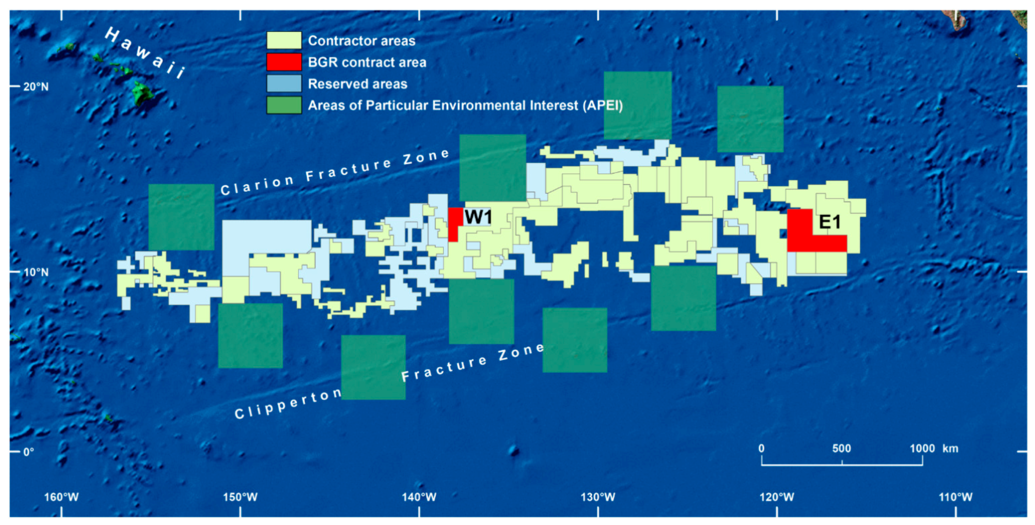
:1. Introduction
2. Exploration Methods
2.1. Strategy Outline
2.2. Multibeam Bathymetry
- Manual, area-based editing of erroneous ping data using SABER software (HMRG);
- Quality control of navigation data (HMRG);
- Manual ping editing of bathymetry using MB-System (BGR).
2.3. Multibeam Backscatter
2.4. Video Surveys
2.5. Box Core Sampling
2.6. Geochemical Analyses of Nodules
2.7. Shear Strength Analysis
2.8. Geostatistical Modelling
- Backscatter (filtered, classified): class 1—sedimentary, flat areas without nodules;
- Backscatter (filtered, classified): class 2—small nodules;
- Backscatter (filtered, classified): class 3—medium-large nodules;
- Backscatter (filtered, classified): class 4—hard reflector;
- Backscatter (z-transformed, filtered): absolute value;
- Bathymetry (filtered): flow accumulation;
- Bathymetry (filtered): slope;
- Bathymetry (z-transformed, filtered): absolute value, inversely scaled;
- Lineaments: Euclidian distance with 15 km maximum;
- Seamounts: Euclidian distance with 13.5 km maximum, inversely scaled;
- Chlorophyll-a concentration: yearly average from spring;
- Temperature of the ocean water surface at night: yearly average from spring;
- Content of particulate organic carbon: yearly average from spring;
- Water current at 4200 m water depth: average of u-vector (W–E direction);
- Water current at 4899 m water depth: average of u-vector;
- Water current at 4200 m water depth: average of v-vector (N–S direction);
- Water current at 4899 m water depth: average of v-vector.
3. Exploration Results
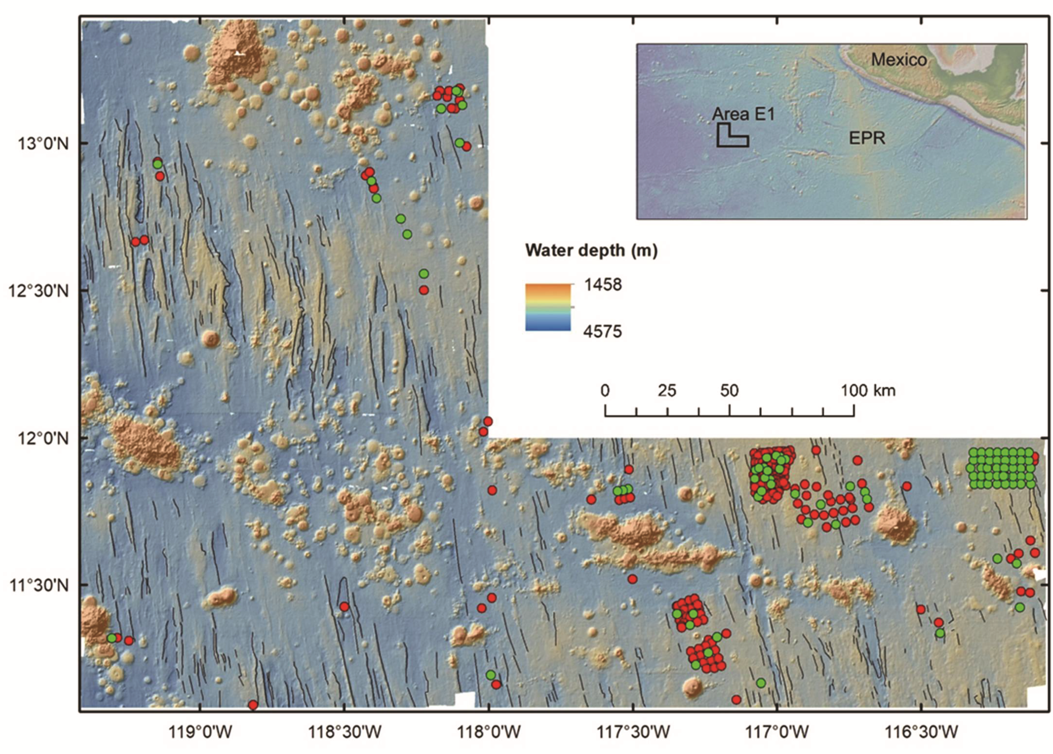
3.1. Geological Setting and Seafloor Topography
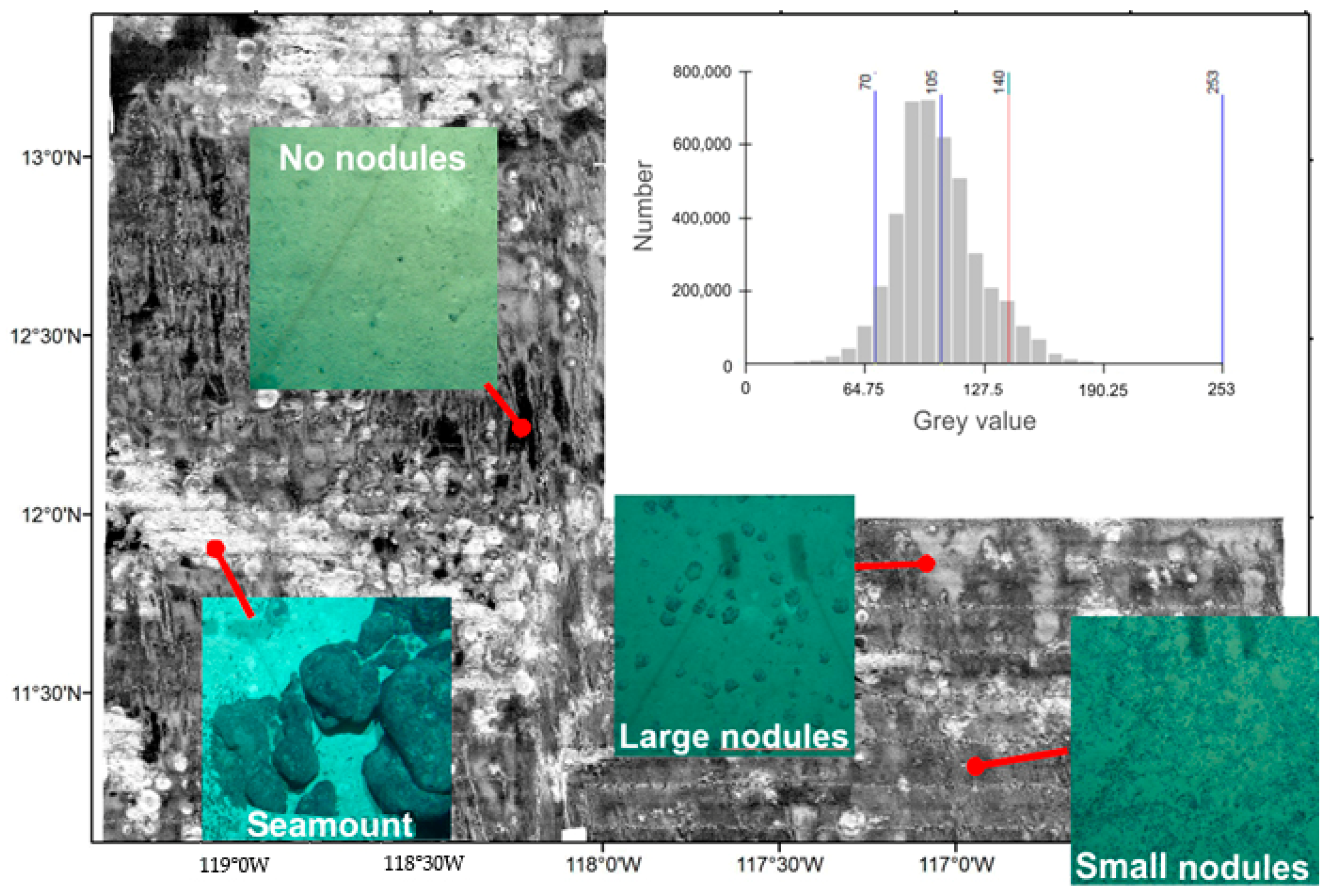
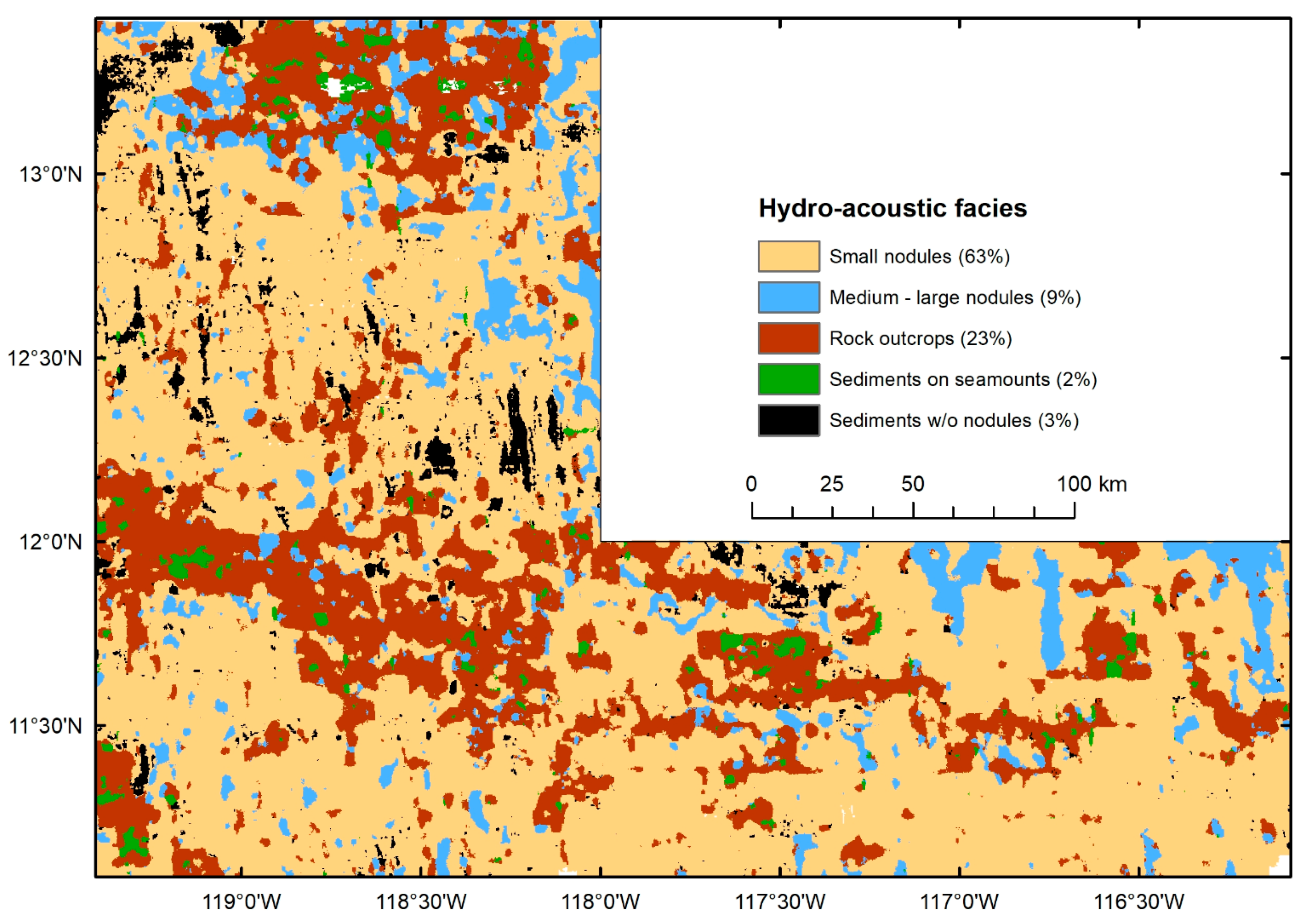
3.2. Backscatter Interpretation
- Class 1 has a very low backscatter strength with grey values between 2 and 70, and it corresponds to a sediment-covered seafloor without nodules. This facies covers about 3% of Area E1.
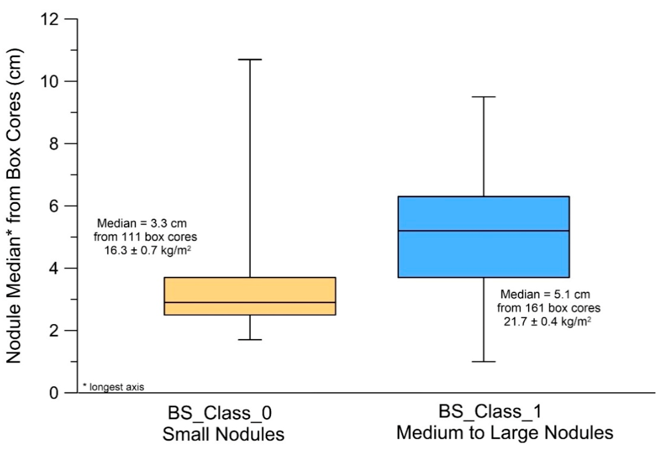
- Class 2 has a low to medium backscatter strength with grey values between 70 and 105 and represents a sediment-covered, flat seafloor with small-sized Mn nodules on top (i.e., nodules having an average diameter of 4 cm or less). In total, 63% of the seafloor is covered by this hydro-acoustic facies.
- Class 3 is characterised by a medium to high backscatter strength between 105 and 140 and is associated with a sediment-covered, flat seafloor and medium- to large-sized Mn nodules with an average diameter of more than 4 cm. Class 3 covers 9% of Area E1.
- Class 4 has a high backscatter strength between 140 and 253 and characterises outcropping hard rocks without sediment cover. This hydro-acoustic class mainly represents the seamounts in Area E1. Some seamounts are flat-topped and covered with sediment. These sediment-covered seamount areas form another hydro-acoustic class, class 5, called “Sediments on seamounts” in Figure 8. However, since seamounts are not a target for future Mn nodule mining, we summarised all seamount areas into hydro-acoustic class 4, which covers 25% of Area E1.
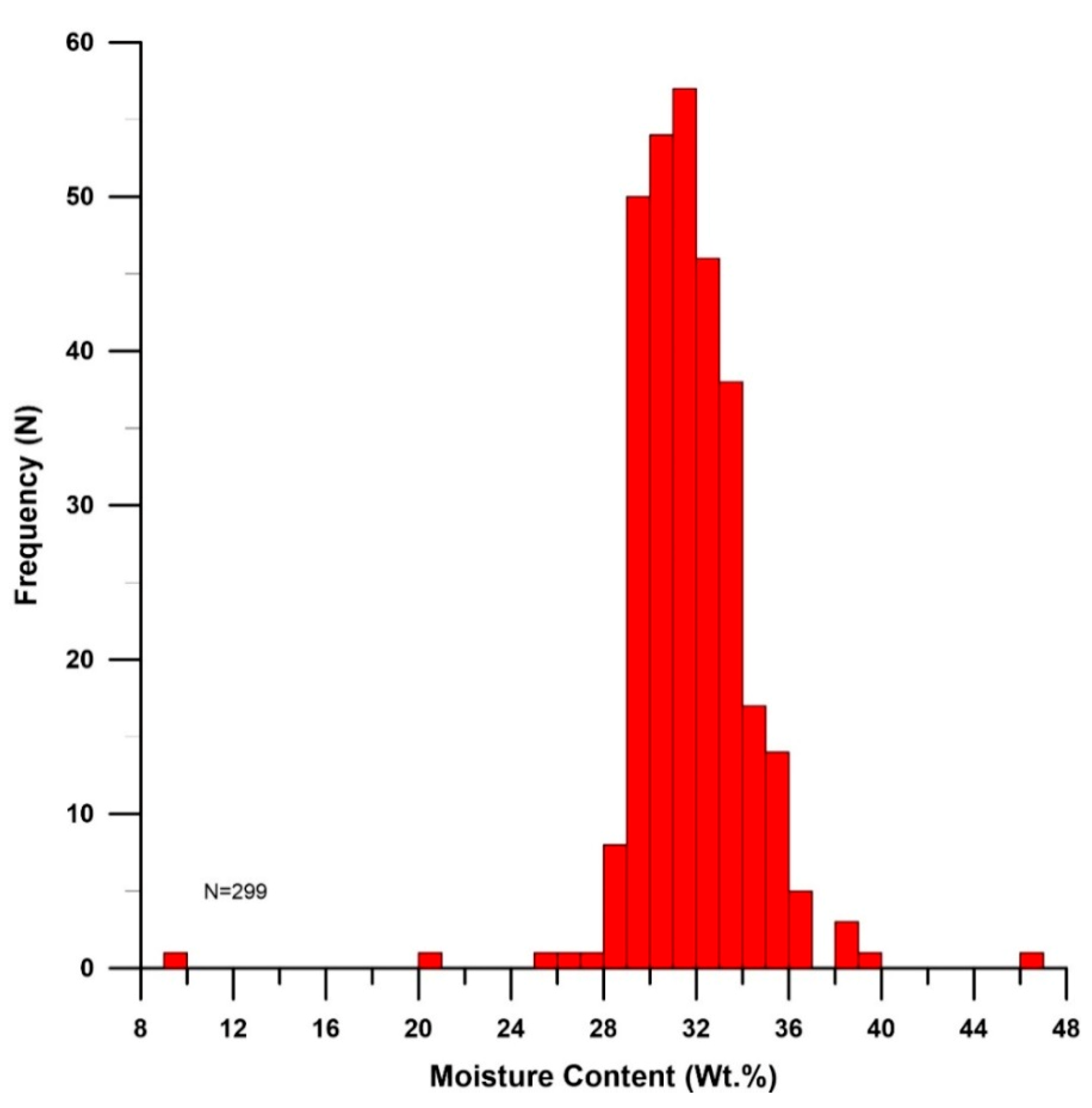
3.3. Physical and Chemical Properties of Surface Sediments
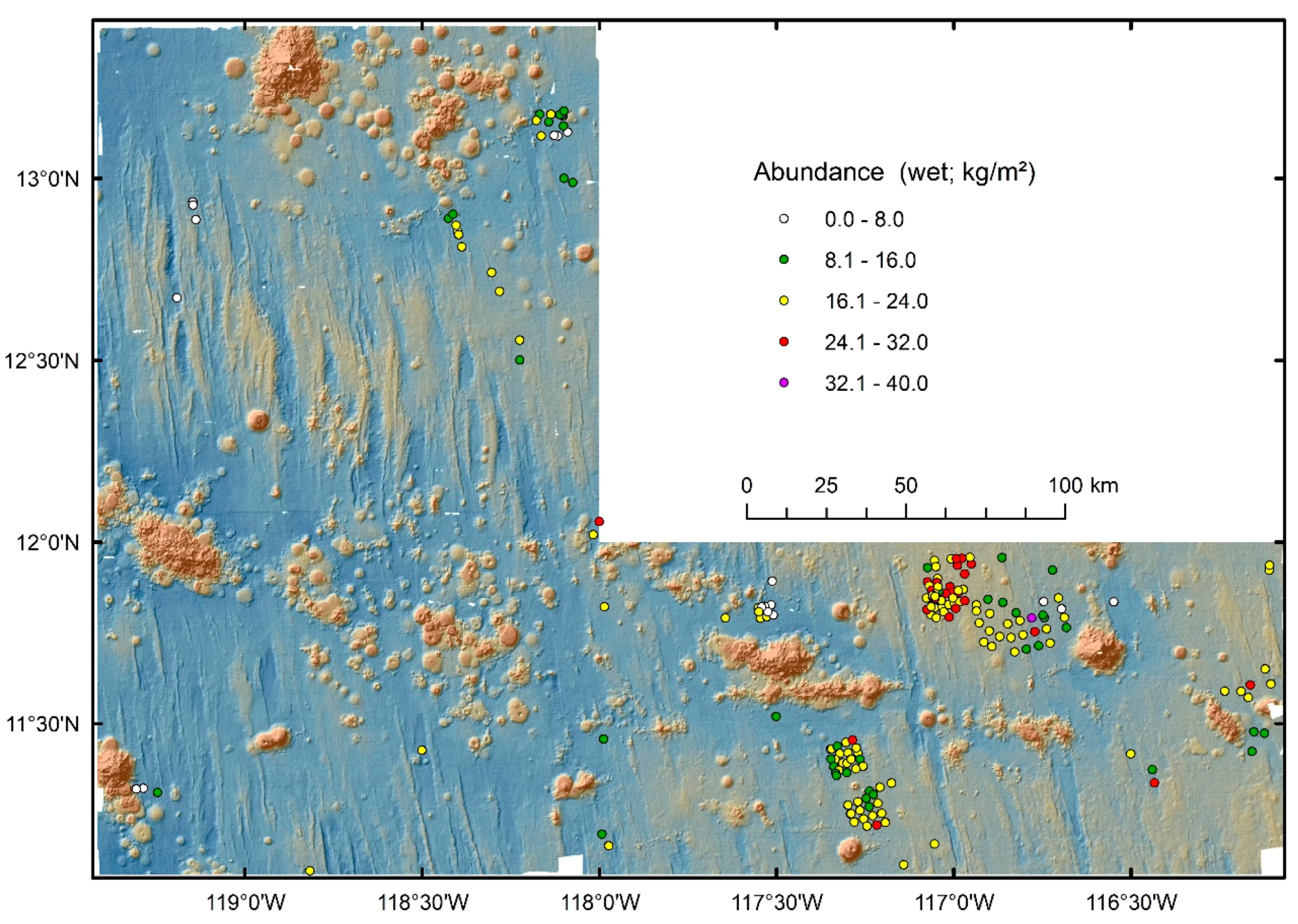
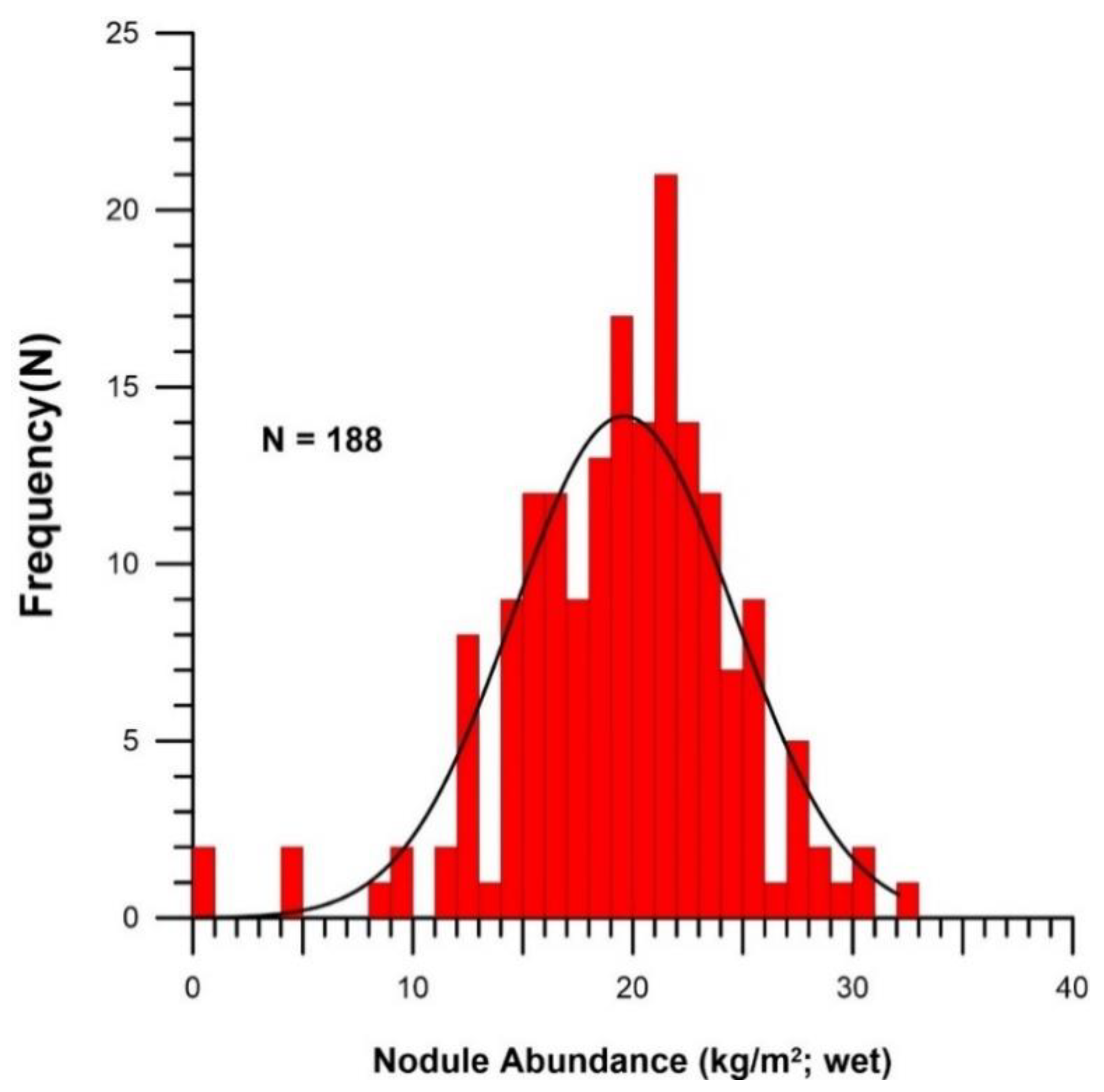
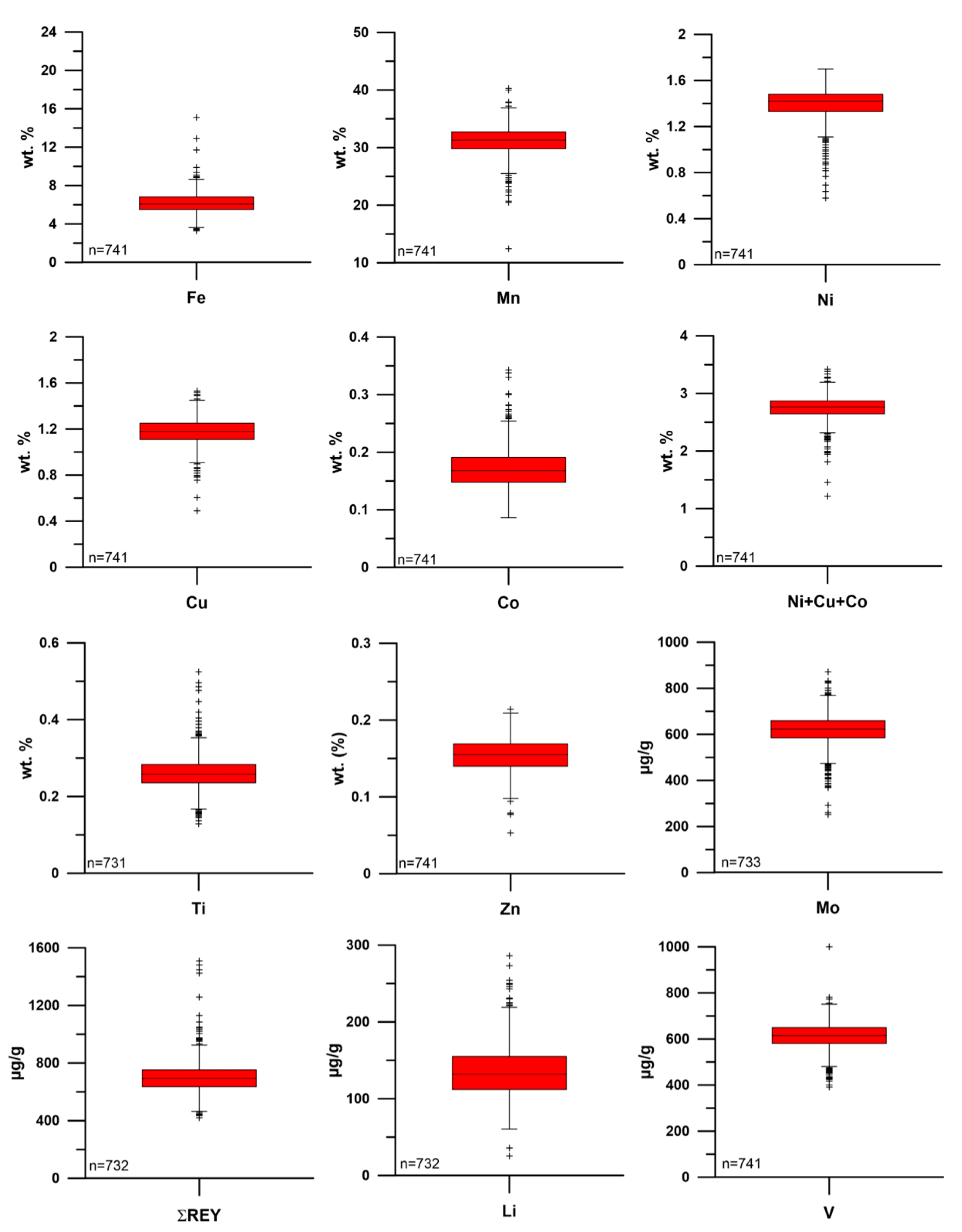
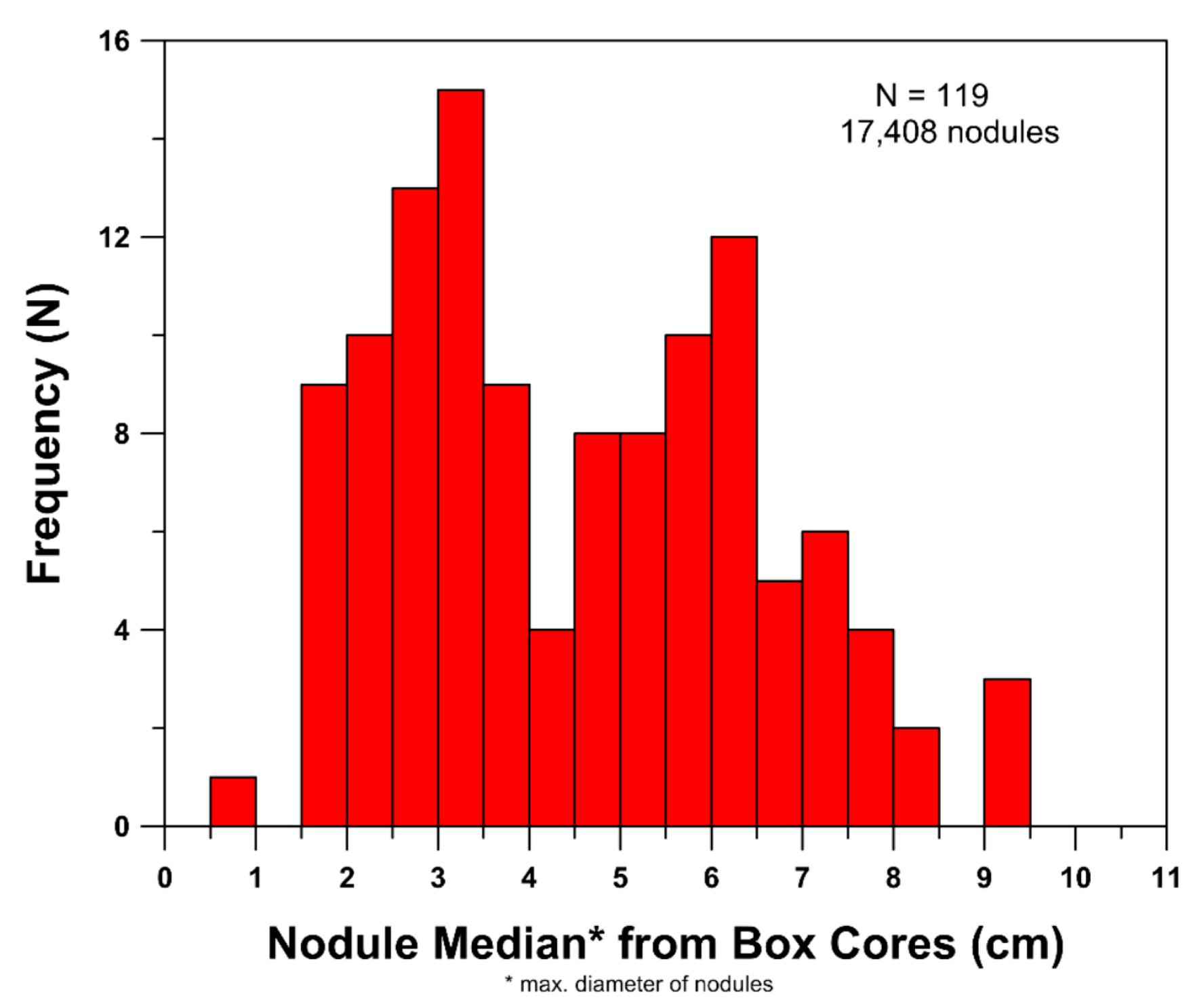
3.4. Nodule Geochemistry, Water Content and Size Distribution
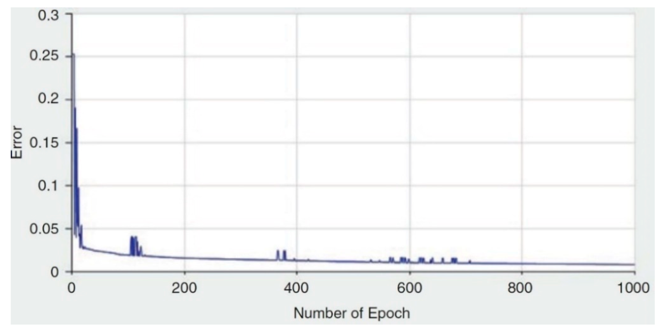
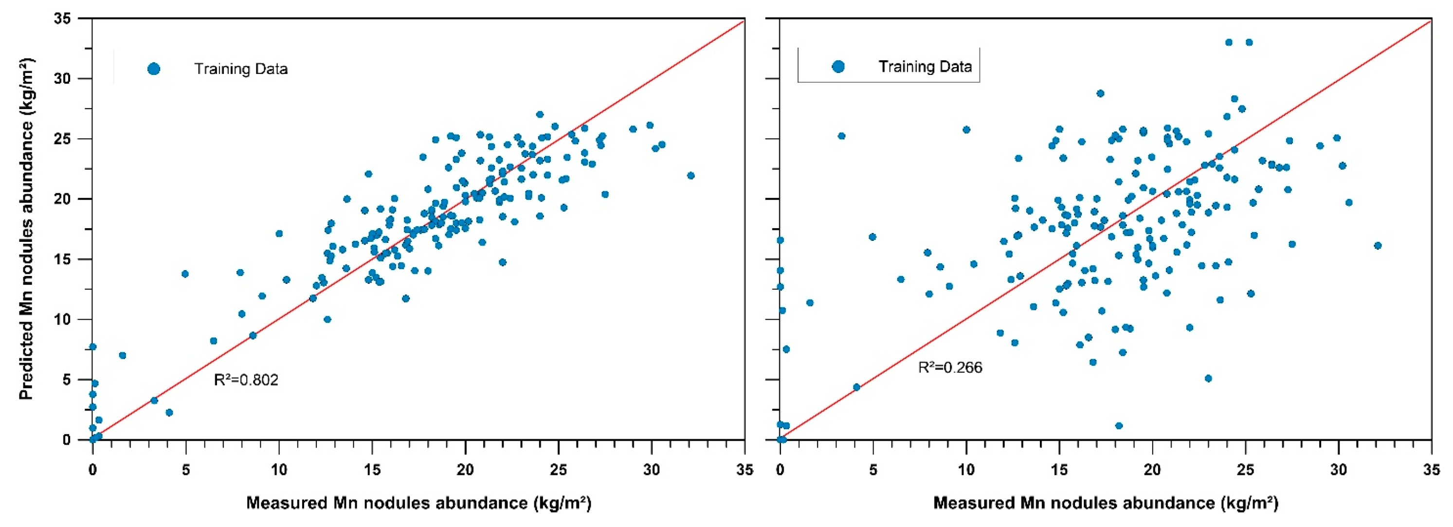
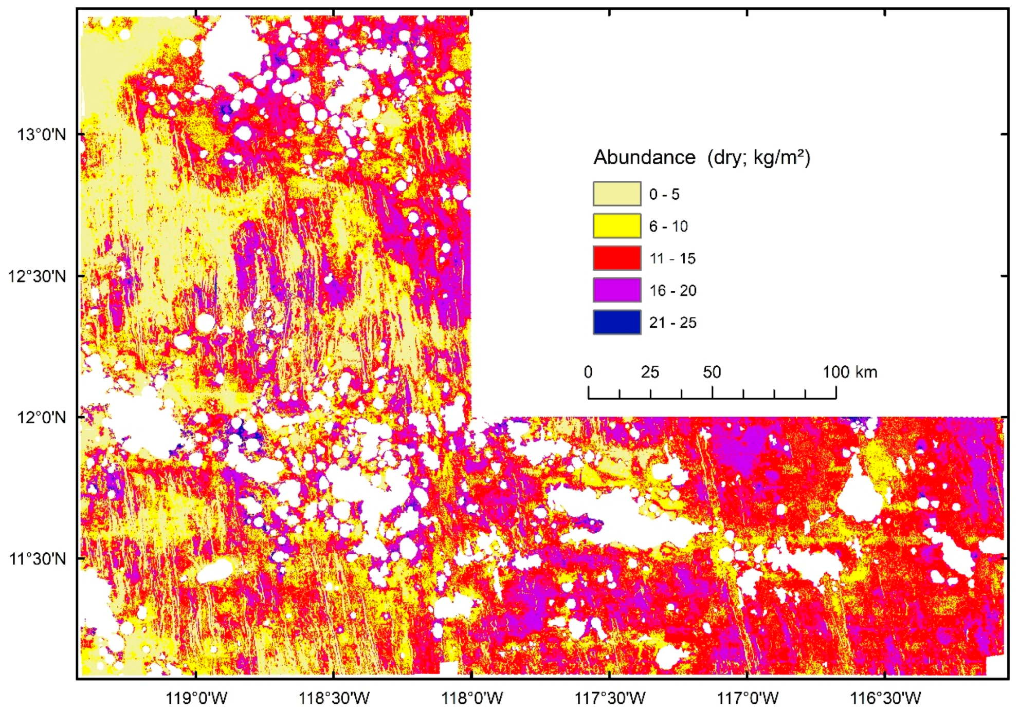
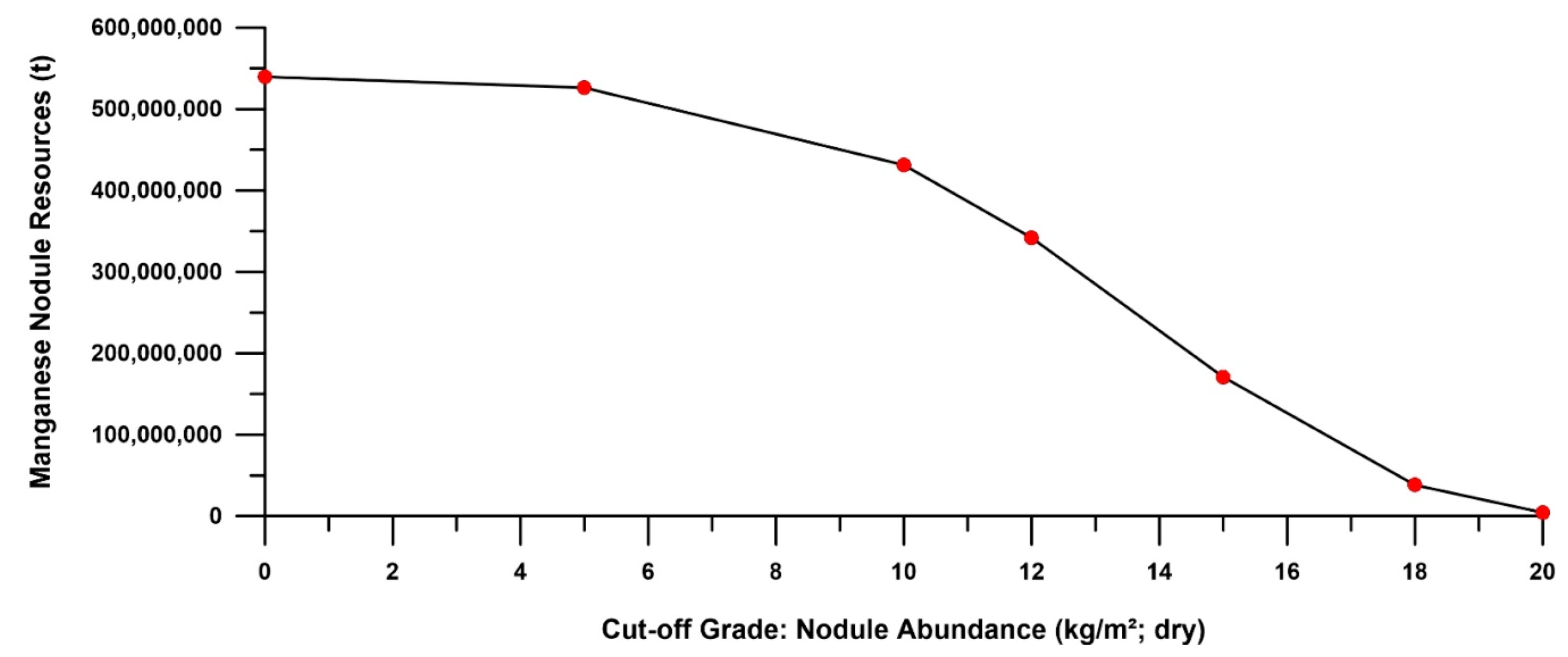
4. Resource Assessment of Area E1 Based on the ANN Model
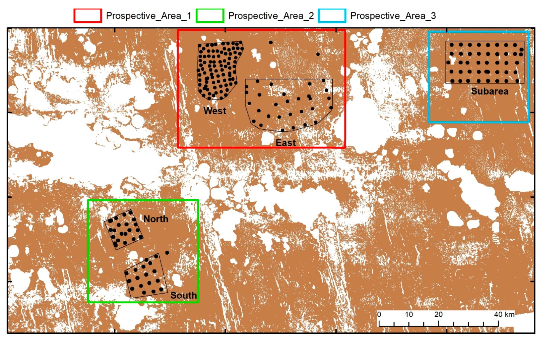
5. Resource Assessment in Prospective Areas
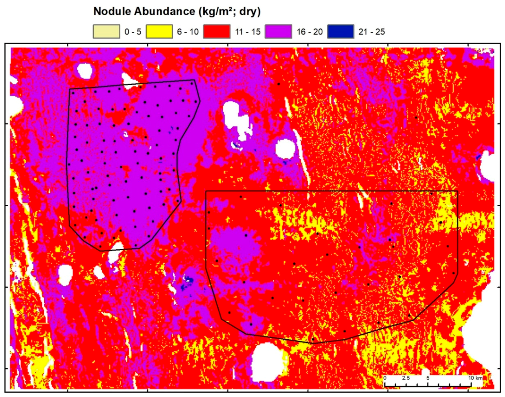
5.1. Description of Data Used for Mineral Resource Estimation
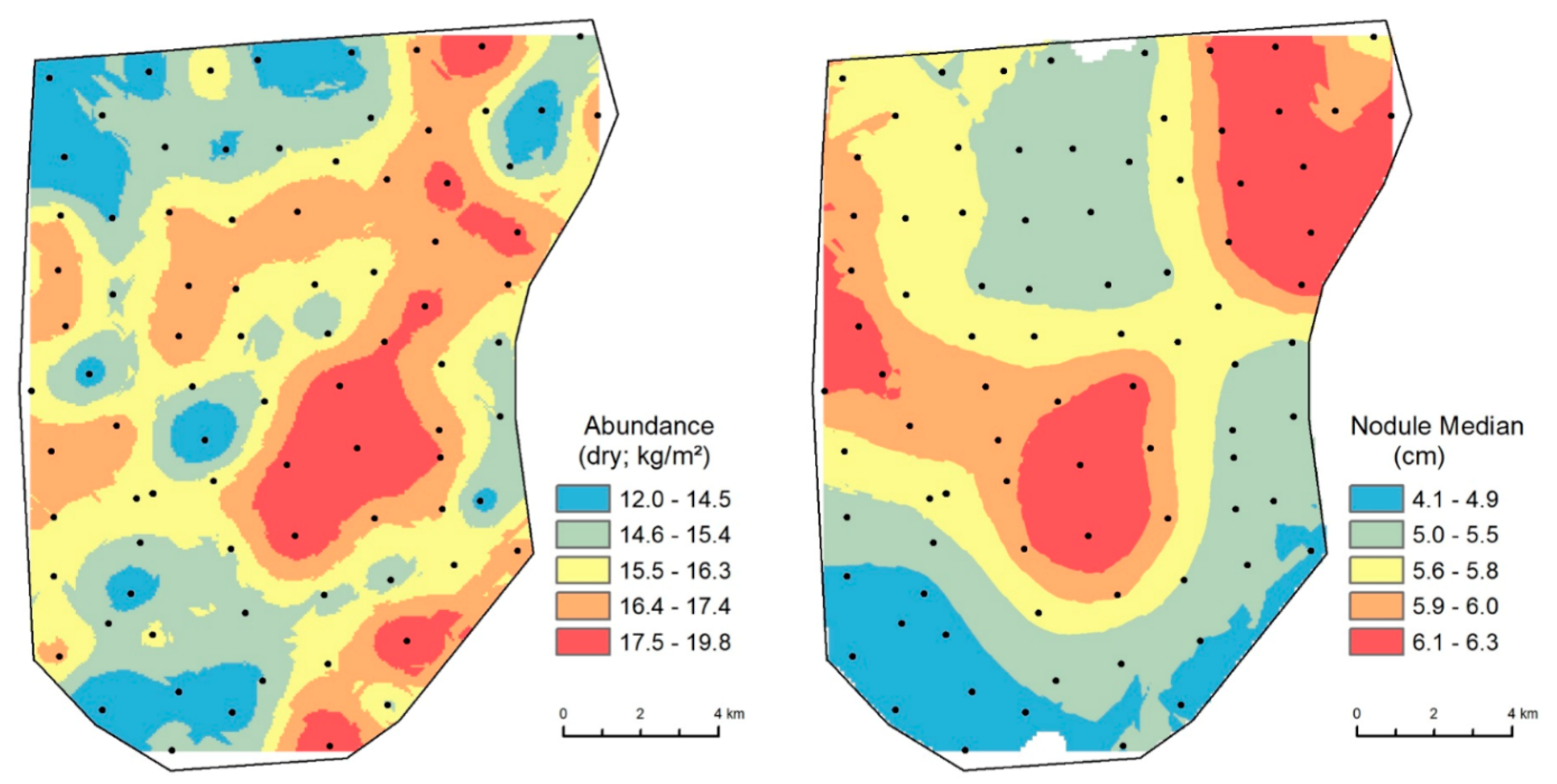
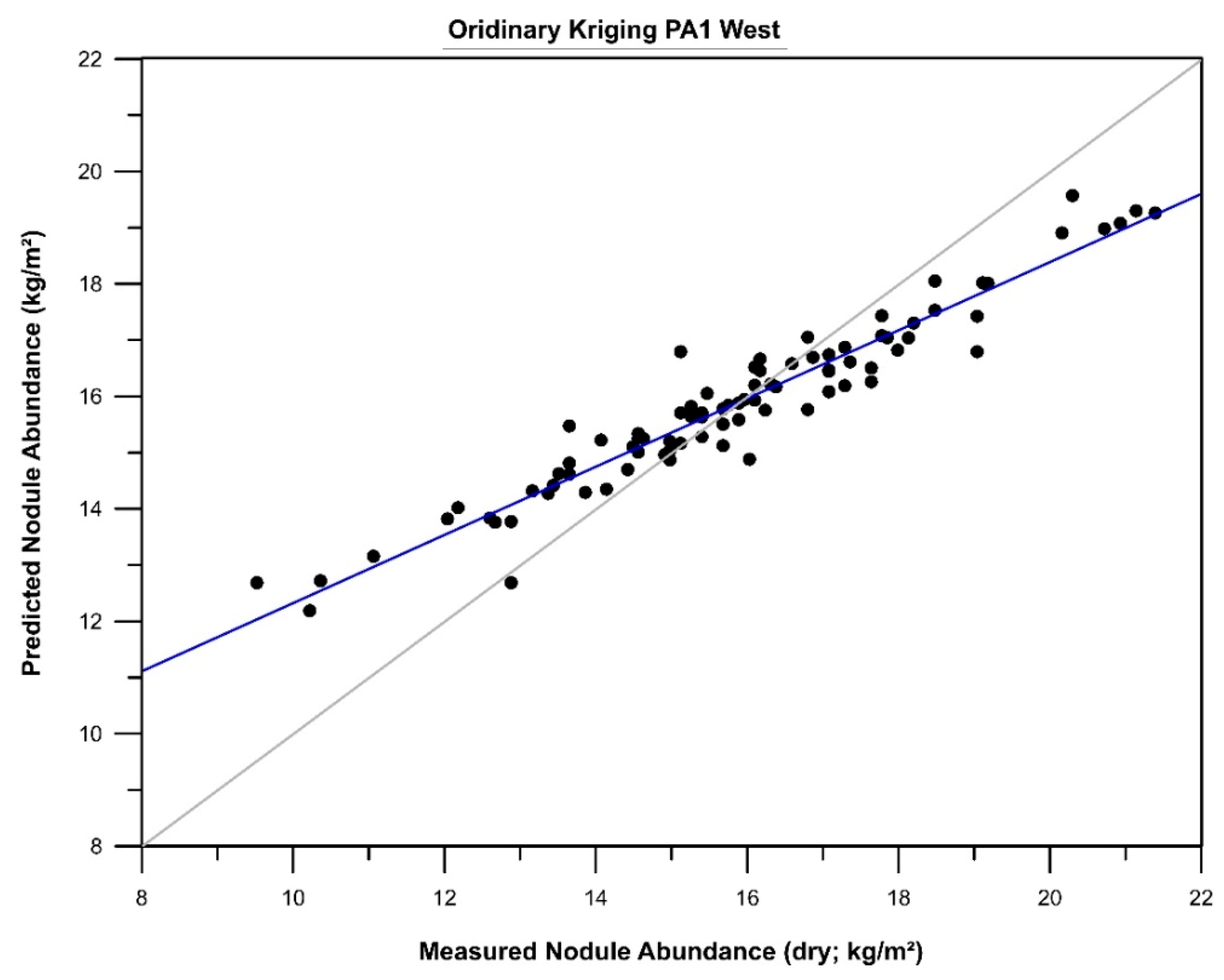
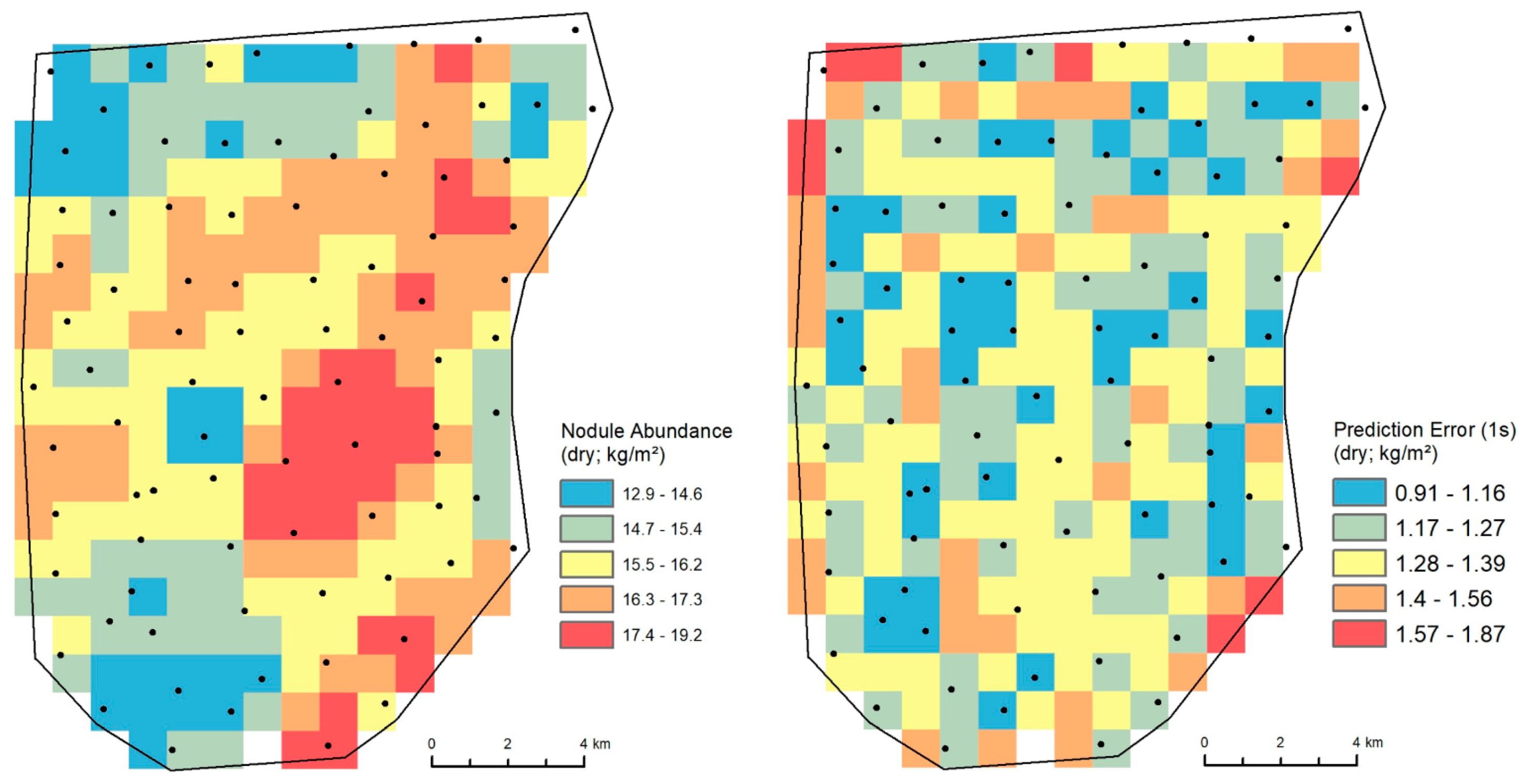
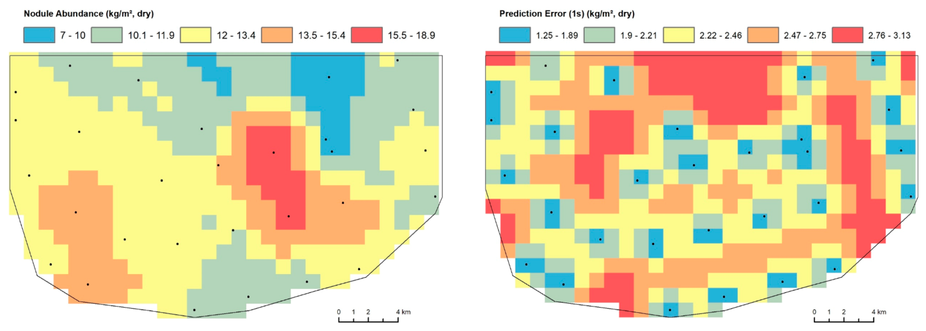
5.2. Resource Estimation for the Western Part of Area PA1 (PA1-West)
5.3. Resource Estimation for the Eastern Part of Area PA1 (PA1-East)
5.4. Resource Estimation for the Entire Area PA1
6. Mineral Resource Classification
7. Conclusions
Author Contributions
Funding
Data Availability Statement
Acknowledgments
Conflicts of Interest
References
- Hein, J.R.; Koschinsky, A.; Kuhn, T. Deep-ocean polymetallic nodules as a resource for critical materials. Nat. Rev. Earth Environ. 2020, 1, 158–169. [Google Scholar] [CrossRef]
- Kuhn, T.; Wegorzewski, A.; Rühlemann, C.; Vink, A. Composition, Formation, and Occurrence of Polymetallic Nodules. In Deep-Sea Mining; Springer Science and Business Media LLC: Berlin/Heidelberg, Germany, 2017; Volume 90, pp. 23–63. [Google Scholar]
- International Seabed Authority. Environmental Assessment and Management for Exploitation of Minerals in the Area; ISA Technical Study No. 16; Kingston: Fountain Valley, CA, USA, 2016; p. 74.
- European Commission. Study on the Review of the List of Critical Raw Materials. Directorate-General for Internal Market, Industry, Entrepreneurship and SMEs; European Commission: Brussels, Belgium, 2017; p. 515. [CrossRef]
- Kuhn, T.; Rühlemann, C.; Wiedicke-Hombach, M. Developing a Strategy for the Exploration of Vast Seafloor Areas for Prospective Manganese Nodule Fields. In Proceedings of the 41st Conference of the Underwater Mining Institute, UMI 2012, Shanghai, China, 15–20 October 2012. [Google Scholar]
- Knobloch, A.; Kuhn, T.; Rühlemann, C.; Hertwig, T.; Zeissler, K.-O.; Noack, S. Predictive Mapping of the Nodule Abundance and Mineral Resource Estimation in the Clarion-Clipperton Zone Using Artificial Neural Networks and Classical Geostatistical Methods. In Deep-Sea Mining; Sharma, R., Ed.; Springer International Publishing: Cham, Switzerland, 2017; Volume 122, pp. 189–212. [Google Scholar]
- Rühlemann, C.; Barckhausen, U.; Ladage, S.; Reinhardt, L.; Wiedicke, M. Exploration for polymetallic nodules in the German license area. In Proceedings of the Eighth (2009) ISOPE Ocean Mining Symposium, Chennai, India, 20–24 September 2009; pp. 8–14. [Google Scholar]
- Schöning, T.; Bergmann, M.; Ontrup, J.; Taylor, J.; Dannheim, J.; Gutt, J.; Purser, A.; Nattkemper, T.W. Semi-automated image analysis for the assessment of megafaunal densities at the Arctic deep-sea observatory HAUSGARTEN. PLoS ONE 2012, 7, e38179. [Google Scholar] [CrossRef] [PubMed] [Green Version]
- Kuhn, T.; Rathke, M. Visual Data Acquisition in the Field and Interpretation for Seafloor Manganese Nodules. EU Project Blue Mining (GA No. 604500) Delivery D1.31. 2017, p. 34. Available online: http//:www.bluemining.eu/downloads (accessed on 14 June 2019).
- Kuhn, T.; Versteegh, G.J.M.; Villinger, H.; Dohrmann, I.; Heller, C.; Koschinsky, A.; Kaul, N.; Ritter, S.; Wegorzewski, A.V.; Kasten, S. Widespread seawater circulation in 18–22 Ma oceanic crust: Impact on heat flow and sediment geochemistry. Geology 2017, 45, 799–802. [Google Scholar] [CrossRef] [Green Version]
- Kriete, C. An Evaluation of the Inter-Method Discrepancies in Ferromanganese Nodule Proficiency Test GeoPT 23A. Geostand. Geoanal. Res. 2011, 35, 319–340. [Google Scholar] [CrossRef]
- Alexander, B.W. Trace Element Analysis in Geological Materials Using Low Resolution Inductively Coupled Plasma Mass Spectrometry (ICPMS); Jacobs University Technical Report No. 18; Jacobs University: Bremen, Germany, 2008. [Google Scholar]
- Hansbo, S. A new approach to the determination of shear strength of clay by the fall-cone test. Proc. R. Swed. Geotech. Inst. 1957, 14, 5–47. [Google Scholar]
- Houlsby, G.T. Theoretical analysis of the fall cone test. Géotechnique 1982, 32, 111–118. [Google Scholar] [CrossRef]
- Kuhn, T.; Heller, C.; Wegorzewski, A. Niedrig-thermale Fluidzirkulation Zwischen Seamounts und Hydrothermalen Senken: Wärmeflusssystem, Einfluss auf Biogeochemische Prozesse und auf das Auftreten und die Zusammensetzung von Manganknollen im Äquatorialen Ostpazifik; Abschlussbericht Projekt SO240—FLUM: Hannover, Germany, 2018; p. 185. [Google Scholar]
- Mewes, K.; Mogollón, J.; Picard, A.; Rühlemann, C.; Kuhn, T.; Nöthen, K.; Kasten, S. Impact of depositional and biogeochemical processes on small scale variations in nodule abundance in the Clarion-Clipperton Fracture Zone. Deep. Sea Res. Part I Oceanogr. Res. Pap. 2014, 91, 125–141. [Google Scholar] [CrossRef]
- Johnson, D.A. Ocean-Floor Erosion in the Equatorial Pacific. GSA Bull. 1972, 83, 3121–3144. [Google Scholar] [CrossRef]
- Rühlemann, C.; Kuhn, T.; Vink, A.; Wiedicke-Hombach, M. Methods of manganese nodule exploration in the German license area. In Recent Developments in Atlantic Seabed Minerals Exploration and Other Topics of Timely Interest; Morgan, C.L., Ed.; The Underwater Mining Institute: Rio de Janeiro, Brazil, 2013; p. 7. [Google Scholar]
- Kuhn, T.; Uhlenkott, K.; Martinez, P.; Vink, A.; Rühlemann, C. Manganese Nodule Fields from the NE Pacific as Benthic Habitats. In Seafloor Geomorphology as Benthic Habitat, 2nd ed.; Harris, P., Baker, E., Eds.; Elsevier: Amsterdam, The Netherlands, 2020; pp. 933–947. [Google Scholar]
- Ehrismann, W.; Walther, H.W. (Eds.) Klassifikation von Lagerstättenvorräten mit Hilfe der Geostatistik: Vorträge Einer Diskussionstagung der Fachsektion Lagerstättenforschung in der GMDB. Schriftenreihe der GDMB 39; Verlag Chemie: Basel, Switzerland, 1983. [Google Scholar]
- Benndorf, J. Vorratsklassifikation nach internationalen Standards—Anforderungen und Modellansätze in der Lagerstattenbearbeitung. Markscheidewesen 2015, 122, 6–14. [Google Scholar]
- CRIRSCO. International Reporting Template for the Public Reporting of Exploration Results, Mineral Resources and Mineral Reserves. Committee for Mineral Reserves International Reporting Standards; ICMM: London, UK, 2013; Available online: http://www.crirsco.com/templates/internation-al_reporting_template_november_2013.pdf (accessed on 23 April 2014).
- International Seabed Authority. Recommendations for the Guidance of Contractors for the Assessment of the Possible Environmental Impacts Arising from Exploration for Marine Minerals in the Area. 2020. Available online: https://isa.org.jm/files/files/documents/26ltc-6-rev1-en_0.pdf (accessed on 17 October 2019).
- Kirchain, R.; Roth, R.; Field, F.R.; Muñoz-Royo, C.; Peacock, T. Report to the International Seabed Authority on the Development of an Economic Model and System of Payments for the Exploitation of Polymetallic Nodules in the Area; Massachusetts Institute of Technology: Cambridge, MA, USA, 2019; p. 77. [Google Scholar]
- Juan, C.; Van Rooij, D.; De Bruycker, W. An assessment of bottom current controlled sedimentation in Pacific Ocean abyssal environments. Mar. Geol. 2018, 403, 20–33. [Google Scholar] [CrossRef]
- Parianos, J.; Lipton, I.; Nimmo, M. Aspects of Estimation and Reporting of Mineral Resources of Seabed Polymetallic Nodules: A Contemporaneous Case Study. Minerals 2021, 11, 200. [Google Scholar] [CrossRef]
- Wasilewska-Błaszczyk, M.; Mucha, J. Possibilities and Limitations of the Use of Seafloor Photographs for Estimating Polymetallic Nodule Resources—Case Study from IOM Area, Pacific Ocean. Minerals 2020, 10, 1123. [Google Scholar] [CrossRef]
- Mucha, J.; Wasilewska-Błaszczyk, M. Estimation Accuracy and Classification of Polymetallic Nodule Resources Based on Classical Sampling Supported by Seafloor Photography (Pacific Ocean, Clarion-Clipperton Fracture Zone, IOM Area). Minerals 2020, 10, 263. [Google Scholar] [CrossRef] [Green Version]
- Yoo, C.M.; Joo, J.; Lee, S.H.; Ko, Y.; Chi, S.-B.; Kim, H.J.; Seo, I.; Hyeong, K. Resource Assessment of Polymetallic Nodules Using Acoustic Backscatter Intensity Data from the Korean Exploration Area, Northeastern Equatorial Pacific. Ocean Sci. J. 2018, 53, 381–394. [Google Scholar] [CrossRef]
- Yang, Y.; He, G.; Ma, J.; Yu, Z.; Yao, H.; Deng, X.; Liu, F.; Wei, Z. Acoustic quantitative analysis of ferromanganese nodules and cobalt-rich crusts distribution areas using EM122 multibeam backscatter data from deep-sea basin to seamount in Western Pacific Ocean. Deep. Sea Res. Part I Oceanogr. Res. Pap. 2020, 161, 103281. [Google Scholar] [CrossRef]


| No. of Measurements | Typical Range of Values | Average Value | Coefficient of Variation (CoV) | |
|---|---|---|---|---|
| Dry bulk density (g/cm3) | 2157 | 0.2–0.6 | 0.34 | 0.22 |
| Shear strength (kPa) | 3571 | 0.5–20 | 4.42 | 0.76 |
| TOC (%) | 2253 | 0.15–0.65 | 0.36 | 0.33 |
| CaCO3 (%) | 2032 | 0–12.7 | 3.51 | 1.63 |
| Metal | Avg. Content (%) ± 1σ | Metal | Avg. Content (μg/g) ± 1σ |
|---|---|---|---|
| Manganese | 31.1 ± 2.56 | Molybdenum | 617 ± 75 |
| Iron | 6.21 ± 1.07 | Lithium | 136 ± 34 |
| Nickel | 1.39 ± 0.14 | ΣREY | 700 ± 117 |
| Copper | 1.17 ± 0.12 | ||
| Cobalt | 0.17 ± 0.03 |
| Cut-Off Dry (kg/m2) | Cut-Off Wet (kg/m2) | Mean Abundance (Dry; kg/m2) | Nodule Resource (Dry; Mt) | Area (km2) | Areal Fraction of E1 (%) |
|---|---|---|---|---|---|
| 0 | 0 | 10.1 | 540 ± 189 | 53,198 | 82 |
| 5 | 7 | 12.3 | 526 ± 184 | 42,973 | 66 |
| 10 | 14 | 14.0 | 431 ± 151 | 30,919 | 48 |
| 12 | 17 | 15.0 | 342 ± 120 | 22,824 | 35 |
| 15 | 21 | 16.9 | 171 ± 60 | 10,093 | 16 |
| 18 | 26 | 18.9 | 38 ± 13 | 2024 | 3.1 |
| 20 | 29 | 20.8 | 4.4 ± 1.5 | 211 | 0.3 |
| Element | Cut-Off Grade Mn Nodule Abundance (Dry, kg/m2) Metal Resource in Area E1 | ||||||
|---|---|---|---|---|---|---|---|
| (t) | 0 kg/m2 | 5 kg/m2 | 10 kg/m2 | 12 kg/m2 | 15 kg/m2 | 18 kg/m2 | 20 kg/m2 |
| Mn | 167,832,487 | 163,646,505 | 134,126,556 | 106,316,718 | 53,129,530 | 11,877,130 | 1,364,041 |
| Ni | 7,501,195 | 7,314,104 | 5,994,724 | 4,751,776 | 2,374,600 | 530,843 | 60,965 |
| Cu | 6,313,955 | 6,156,476 | 5,045,919 | 3,999,696 | 1,998,764 | 446,825 | 51,316 |
| Ti | 1,403,101 | 1,368,106 | 1,121,315 | 888,821 | 444,170 | 99,294 | 11,404 |
| Co | 917,412 | 894,531 | 733,168 | 581,152 | 290,419 | 64,923 | 7456 |
| Zn | 809,481 | 789,292 | 646,913 | 512,782 | 256,252 | 57,285 | 6579 |
| REY 1 | 377,758 | 368,336 | 301,893 | 239,298 | 119,584 | 26,733 | 3070 |
| V | 330,268 | 322,031 | 263,940 | 209,215 | 104,551 | 23,372 | 2684 |
| Mo | 332,967 | 324,662 | 266,097 | 210,924 | 105,405 | 23,563 | 2706 |
| Ga | 14,031 | 13,681 | 11,213 | 8888 | 4442 | 993 | 114 |
| Variable | Samples | Min. | Max. | Mean | Median | StdDev | CoV (%) |
|---|---|---|---|---|---|---|---|
| Abundance 1 (kg/m2) | 93 | 9.52 | 36.3 | 16.2 | 15.9 | 3.46 | 21 |
| Mn (%) | 81 | 27.0 | 34.0 | 31.5 | 31.8 | 1.54 | 5 |
| Ni (%) | 81 | 1.24 | 1.59 | 1.44 | 1.45 | 0.09 | 6 |
| Cu (%) | 81 | 1.01 | 1.36 | 1.20 | 1.20 | 0.07 | 6 |
| Co (%) | 81 | 0.12 | 0.19 | 0.16 | 0.16 | 0.01 | 9 |
| Mo (µg/g) | 79 | 466 | 697 | 601 | 609 | 45 | 7 |
| ƩREY 2 (µg/g) | 79 | 530 | 824 | 658 | 673 | 65 | 10 |
| Li (µg/g) | 79 | 123 | 202 | 150 | 150 | 16 | 10 |
| Nodule Median (cm) | 90 | 3.0 | 9.1 | 5.62 | 5.80 | 1.40 | 25 |
| Variable | C0 (Nugget) | % of Total Sill | C1 (Partial Sill) | % of Total Sill | Range (m) | Resource 1 (t) | Uncertainty 1 (t) |
|---|---|---|---|---|---|---|---|
| Abundance | 2.0 | 37 | 3.4 | 63 | 2500 | 3,780,000 | ±600,000 |
| Mn | 1.0 | 40 | 1.5 | 60 | 2500 | 1,190,000 | ±260,000 |
| Ni | 0.005 | 59 | 0.0035 | 41 | 6000 | 54,126 | ±11,366 |
| Cu | 0.002 | 38 | 0.0033 | 62 | 5000 | 45,336 | ±9521 |
| Co | 0.00008 | 40 | 0.00012 | 60 | 4300 | 5948 | ±1487 |
| Mo | n.a. 2 | n.a. 2 | n.a. 2 | 2265 | ±317 | ||
| ƩREY | 2056 | 46 | 2450 | 54 | 6300 | 2473 | ±618 |
| Li | 66 | 22 | 228 | 78 | 4100 | 567 | ±153 |
| Block Size (m) | Number of Blocks | Area (km2) | Resource (Mt; Dry) | Absolute Error (Mt) 1 | Relative Error (%) 1 |
|---|---|---|---|---|---|
| 100 | 23,532 | 235 | 3.75 | ±0.72 | 19.2 |
| 500 | 952 | 238 | 3.79 | ±0.68 | 17.9 |
| 1000 | 237 | 237 | 3.78 | ±0.60 | 16.0 |
| 2000 | 64 | 256 | 4.08 | ±0.26 | 12.9 |
| 5000 | 10 | 250 | 3.95 | ±0.20 | 10.2 |
| ANN model 2 | 23,532 | 235 | 3.92 | ±1.06/±1.37 3 | 27/35 3 |
| Variable | Samples | Min. | Max. | Mean | Median | StdDev | CoV (%) |
|---|---|---|---|---|---|---|---|
| Abundance 1 (kg/m2) | 30 | 5.54 | 22.5 | 12.1 | 11.9 | 3.37 | 28 |
| Mn (wt.%) | 30 | 28.6 | 33.1 | 31.5 | 31.9 | 1.16 | 3.7 |
| Ni (wt.%) | 30 | 1.22 | 1.55 | 1.43 | 1.43 | 0.07 | 4.9 |
| Cu (wt.%) | 30 | 1.01 | 1.43 | 1.15 | 1.12 | 0.10 | 8.7 |
| Co (wt.%) | 30 | 0.15 | 0.22 | 0.18 | 0.18 | 0.018 | 10 |
| Mo (µg/g) | 29 | 566 | 688 | 621 | 617 | 36 | 5.2 |
| ƩREY 2 (µg/g) | 29 | 578 | 828 | 724 | 751 | 71 | 10 |
| Li (µg/g) | 29 | 98 | 195 | 130 | 129 | 20 | 15 |
| Nodule Median (cm) | 29 | 2.00 | 7.25 | 3.66 | 3.10 | 1.41 | 39 |
| Variable | C0 (Nugget) | % of Total Sill | C1 (Partial Sill) | % of Total Sill | Range (m) | Resource 1 (t) | Uncertainty 1 (t) |
|---|---|---|---|---|---|---|---|
| Nod. abund. | 2.50 | 22 | 9.05 | 78 | 5000 | 5,750,000 | 2,220,000 |
| Mn | 0 | 0 | 1.11 | 100 | 8000 | 1,810,000 | 760,000 |
| Ni | 0.0035 | 58 | 0.0025 | 42 | 7000 | 82,481 | 36,456 |
| Cu | 0.002 | 18 | 0.0089 | 82 | 10,000 | 66,832 | 32,013 |
| Co | 1.1 × 10⁻⁴ | 31 | 2.5 × 10⁻⁴ | 69 | 8300 | 10,528 | 5264 |
| Mo | n.a. 2 | n.a. | n.a. | 3449 | 1725 | ||
| ƩREY | 0 | 0 | 5453 | 100 | 9800 | 4142 | 1988 |
| Li | 150 | 37 | 260 | 63 | 9000 | 744 | 417 |
| Area | Tonnage 1 km2 Blocks Mt (Wet) | Uncertainty 1 1 km2 Blocks Mt (Wet) | Tonnage 1 km2 Blocks Mt (Dry) | Uncertainty 1 1 km2 Blocks Mt (Dry) | Area (km2) | Area2 1000 m blocks (km2) | Uncertainty (%) 1 | ||||
|---|---|---|---|---|---|---|---|---|---|---|---|
| 100 3 m | 500 m | 1000 m | 2000 m | 5000 m | |||||||
| PA1-West | 5.40 | ±0.86 | 3.78 | ±0.60 | 241 | 237 | 19 | 18 | 16 | 13 | 10 |
| PA1-East | 8.22 | ±3.17 | 5.75 | ±2.22 | 450 | 461 | 42 | 40 | 38 | 35 | 26 |
| PA1 | 37.5 | ±13.1 | 26.2 | ±9.2 | 2218 | 2218 | 35 | n.a. | n.a. | n.a. | n.a. |
| PA2-North | 1.96 | ±0.39 | 1.37 | ±0.27 | 103 | 104 | 23 | 21 | 20 | n.a. | n.a. |
| PA2-South | 2.84 | ±0.50 | 1.99 | ±0.35 | 145 | 147 | 19 | 18 | 17 | 16 | n.a. |
| PA2 | 20.6 | ±7.29 | 14.4 | ±5.10 | 1270 | 1270 | 35 | n.a. | n.a. | n.a. | n.a. |
| PA3-Subarea | 7.80 | ±2.56 | 5.46 | ±1.79 | 375 | 375 | 33 | n.a. | n.a. | n.a. | n.a. |
| PA3 | 18.9 | ±6.57 | 13.2 | ±4.60 | 1010 | 1010 | 35 | ||||
| Area | Range Value (m) | Average Sample Distance (m) | Resource | ||
|---|---|---|---|---|---|
| Classification GDMB 1 | Range Value 2 | CRIRSCO 3 | |||
| PA1-West | 2500 | 1315 | indicated | indicated | measured |
| PA1-East | 5000 | 3068 | inferred | indicated | indicated |
| PA1 | n.a. | n.a. | inferred | n.a. | inferred |
| PA2-North | 4726 | 1664 | indicated | measured | measured |
| PA2-South | 6600 | 2078 | indicated | measured | measured |
| PA2 | n.a. | n.a. | inferred | n.a. | inferred |
| PA3-Subarea | 4500 | 2720 | inferred | indicated | indicated |
| PA3 | n.a. | n.a. | inferred | n.a. | inferred |
| Mineral Resource Classification | Abundance (kg/m2; dry) 1 | Area (km2) | Mn (%) | Ni (%) | Cu (%) | Co (%) | Polymetallic Nodules (Dry Mt) |
|---|---|---|---|---|---|---|---|
| Measured | 14.6 | 489 | 31.5 | 1.43 | 1.19 | 0.17 | 7.14 |
| Indicated | 14.2 | 825 | 30.8 | 1.32 | 1.18 | 0.13 | 11.21 |
| Inferred 2 | 13.4 | 3184 | 31.1 | 1.39 | 1.17 | 0.17 | 35.53 |
| Inferred 3 | 10.1 | 60,216 | 31.1 | 1.39 | 1.17 | 0.17 | 486.2 |
Publisher’s Note: MDPI stays neutral with regard to jurisdictional claims in published maps and institutional affiliations. |
© 2021 by the authors. Licensee MDPI, Basel, Switzerland. This article is an open access article distributed under the terms and conditions of the Creative Commons Attribution (CC BY) license (https://creativecommons.org/licenses/by/4.0/).
Share and Cite
Kuhn, T.; Rühlemann, C. Exploration of Polymetallic Nodules and Resource Assessment: A Case Study from the German Contract Area in the Clarion-Clipperton Zone of the Tropical Northeast Pacific. Minerals 2021, 11, 618. https://doi.org/10.3390/min11060618
Kuhn T, Rühlemann C. Exploration of Polymetallic Nodules and Resource Assessment: A Case Study from the German Contract Area in the Clarion-Clipperton Zone of the Tropical Northeast Pacific. Minerals. 2021; 11(6):618. https://doi.org/10.3390/min11060618
Chicago/Turabian StyleKuhn, Thomas, and Carsten Rühlemann. 2021. "Exploration of Polymetallic Nodules and Resource Assessment: A Case Study from the German Contract Area in the Clarion-Clipperton Zone of the Tropical Northeast Pacific" Minerals 11, no. 6: 618. https://doi.org/10.3390/min11060618